Super-Resolution Reconstruction of Remote Sensing Images Using Multifractal Analysis

Abstract
:1. Introduction
2. Methods
2.1. Multifractal Analysis
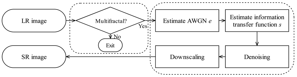
2.2. Super-Resolution Reconstruction
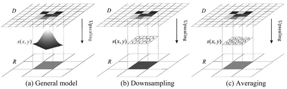
2.2.1. Information transfer function (ITF)
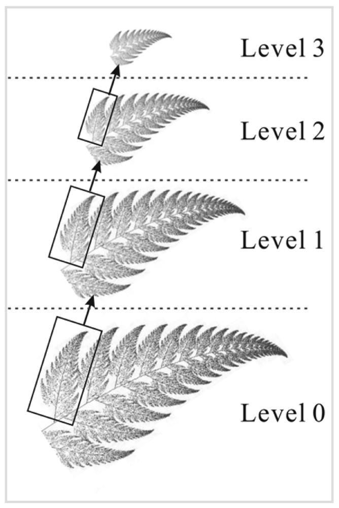
2.2.2. Fractal encoding
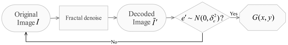
2.2.3. Image denoising
2.2.4. Fractal decoding and downscaling
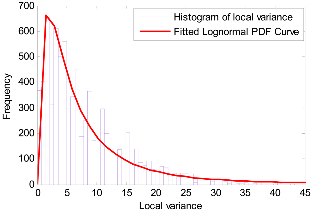
2.3. Parameter Estimation
3. Empirical Study
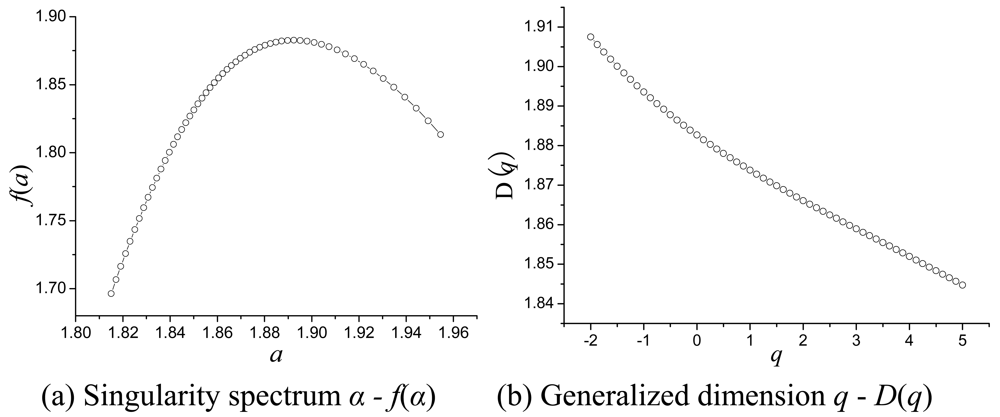
3.1. Multifractal Characteristic
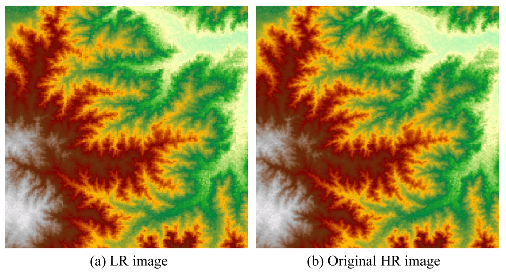
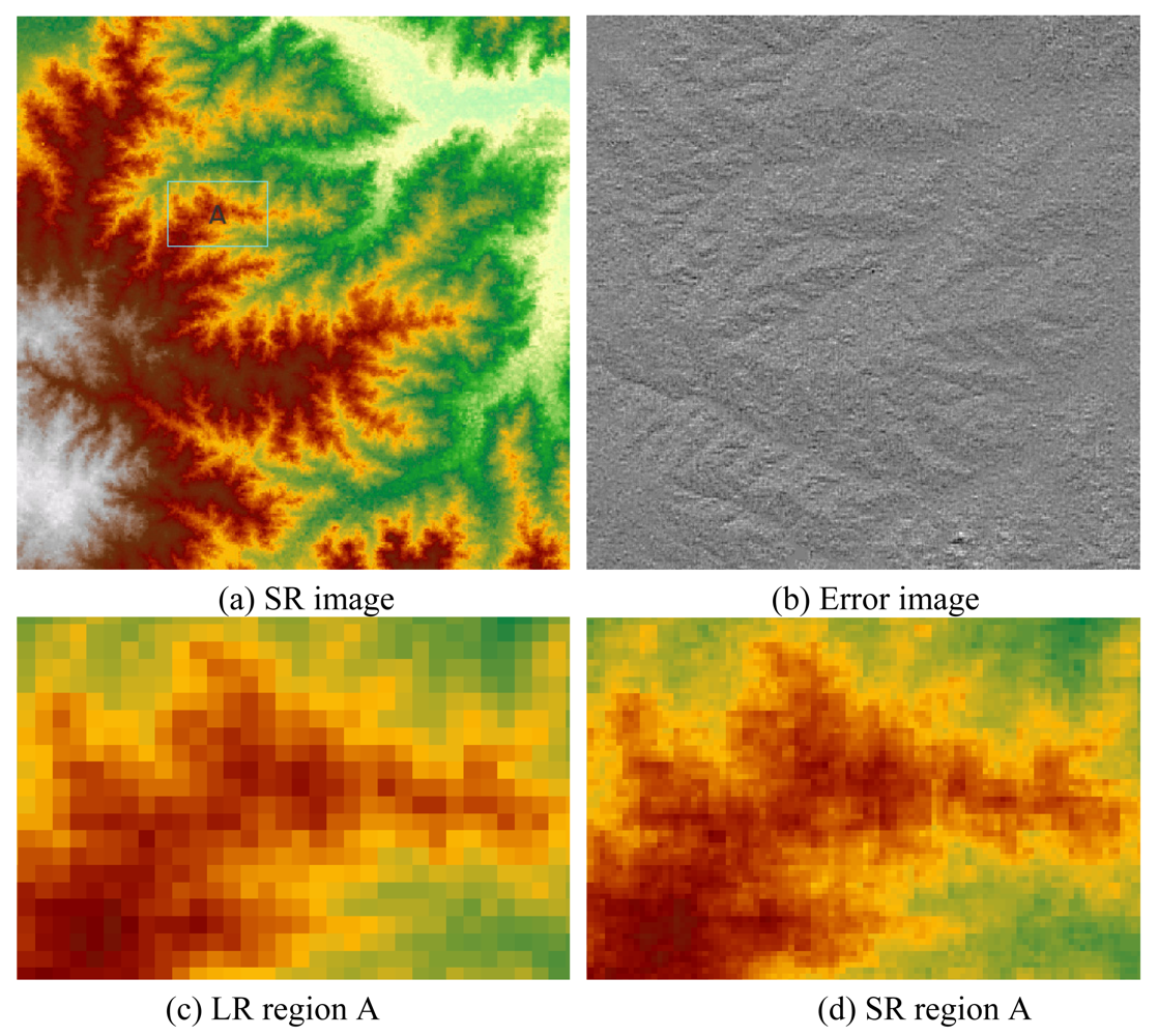
3.2. Super-Resolution Images
4. Discussion and Conclusions
Acknowledgments
References and Notes
- Park, S.C.; Park, M.K.; Kang, A.M.G. Super-resolution image reconstruction: a technical overview. IEEE Signal Process. Mag. 2003, 20, 21–36. [Google Scholar]
- Chaudhuri, S.; Joshi, M.V. Motion-free Super-resolution; Springer: New York, NY, USA, 2005. [Google Scholar]
- Hunt, B.R. Super-resolution of images: algorithms, principles, performance. Int. J. Imaging Syst. Technol. 1995, 6, 297–304. [Google Scholar]
- Candocia, F.M.; Principe, J.C. Super-resolution of images based on local correlations. IEEE Trans. Neural Netw. 1999, 10, 372–380. [Google Scholar]
- Elad, M.; Feuer, A. Restoration of a single superresolution image from several blurred, noisy, and undersampled measured images. IEEE Trans. Image Process 1997, 6, 1646–1658. [Google Scholar]
- Jiji, C.V.; Chaudhuri, S. Single-frame image super-resolution through contourlet learning. EURASIP J. Appl. Signal Process 2006, 2006, 1–11. [Google Scholar]
- Kasetkasem, T.; Arora, M.K.; Varshney, P.K. Super-resolution land cover mapping using a Markov random field based approach. Remote Sen. Environ. 2005, 96, 302–314. [Google Scholar]
- Tsai, R.Y.; Huang, T.S. Multiframe Image Restoration and Registration. In Advances in Computer Vision and Image Processing; JAI Press: Greenwich, UK, 1984; pp. 317–339. [Google Scholar]
- Atkinson, P.M.; Cutler, M.E.J.; Lewis, H. Mapping sub-pixel proportional land cover with AVHRR imagery. Int. J. Remote Sens. 1997, 18, 917–935. [Google Scholar]
- Powell, R.L.; Roberts, D.A.; Dennison, P.E.; Hess, L.L. Sub-pixel mapping of urban land cover using multiple endmember spectral mixture analysis: Manaus, Brazil. Remote Sens. Environ. 2007, 106, 253–267. [Google Scholar]
- Boucher, A.; Kyriakidis, P.C. Super-resolution land cover mapping with indicator geostatistics. Remote Sens. Environ. 2006, 104, 264–282. [Google Scholar]
- Carpenter, G.A.; Gopal, S.; Macomber, S.; Martens, S.; Woodcock, C.E.; Franklin, J. A neural network method for efficient vegetation mapping. Remote Sens. Environ. 1999, 70, 326–338. [Google Scholar]
- Ge, Y.; Li, S.; Lakhan, V.C. Development and testing of a subpixel mapping algorithm. IEEE Trans. Geosci. Remot Sen. 2009, 47, 2155–2164. [Google Scholar]
- Barnsley, M.F.; Sloan, A.D. A better way to compress images. Byte 1988, 13, 215–223. [Google Scholar]
- Varotsos, C.A.; Milinevsky, G.; Grytsai, A.; Efstathiou, M.; Tzanis, C. Scaling effect in planetary waves over Antarctica. Int. J. Remote Sens. 2008, 29, 2697–2704. [Google Scholar]
- Lovejoy, S.; Schertzer, D. Scale Invariance, Symmetries, Fractals, and Stochastic Simulations of Atmospheric Phenomena. Bull. Amer. Meteorol. Soc. 1986, 67, 21–32. [Google Scholar]
- Jacquin, A.E. Image coding based on a fractal theory of iterated contractive image transformations. IEEE Trans. Image Process 1992, 1, 18–30. [Google Scholar]
- Pentland, A.P. Fractal-based description of natural scenes. IEEE Trans. Patt. Anal. Mach. Int. 1984, 6, 661–674. [Google Scholar]
- Lin, H.; Venetsanopoulos, A. Fast fractal image coding using pyramids. In Image Analysis and Processing, Proceedings of 13th International Conference on Image Analysis and Processing, ICIAP 2005, Cagliari, Italy, September, 2005; pp. 649–654.
- Vatolin, D.S. Using DCT for a fractal image compression optimization. Program. Comput. Softw. 1999, 25, 158–164. [Google Scholar]
- Dekeyser, F.; Bouthemy, P.; Perez, P. A New Algorithm for Super-Resolution from Image Sequences. In Computer Analysis of Images and Patterns; Springer: Heidelberg, Germany, 2001; pp. 473–481. [Google Scholar]
- Barnsley, M. Fractals Everywhere; Academic Press Inc.: Burlington, MA, USA, 1988. [Google Scholar]
- Chhabra, A.B.; Meneveau, C.; Jensen, R.V.; Sreenivasan, K.R. Direct determination of the f(α) singularity spectrum and its application to fully developed turbulence. Phys. Rev. A 1989, 40, 5284–5294. [Google Scholar]
- Chlouverakis, K.E.; Sprott, J.C. A comparison of correlation and Lyapunov dimensions. Physica D 2005, 200, 156–164. [Google Scholar]
- Chen, Y.; Luo, Y.; Hu, D. Image superresolution using fractal coding. Opt. Eng. 2008, 47, 1–12. [Google Scholar]
- Ghazel, M.; Freeman, G.H.; Vrscay, E.R. Fractal image denoising. IEEE Trans. Image Process 2003, 12, 1560–1578. [Google Scholar]
- Posadas, A.N.D.; Quiroz, R.; Zorogastua, P.E.; Leon-velarde, C. Multifractal characterization of the spatial distribution of ulexite in a Bolivian salt flat. Int. J. Remote Sens. 2005, 26, 615–627. [Google Scholar]
- Comer, M.L.; Delp, E.J. Segmentation of textured images using a multiresolution Gaussian autoregressive model. IEEE Trans. Image Process 1999, 8, 408–420. [Google Scholar]
- Illgner, K.; Muller, F. Spatially scalable video compression employing resolution pyramids. IEEE J. Sel. Area. Commun 1997, 15, 1688–1703. [Google Scholar]
- Wang, Y.; Zhu, S.C. Perceptual scale-space and its applications. Int. J. Comput. Vision 2008, 80, 143–165. [Google Scholar]
- Wang, Z.; Yu, Y.-L. Partial iterated function system based fractal image coding, Proceedings of SPIE Symposium on Aerospace: Hybrid Image and Signal Processing, Orlando, FL, USA; 1996; pp. 42–49.
- Luedeling, E.; Siebert, S.; Buerkert, A. Filling the voids in the SRTM elevation model−A TIN-based delta surface approach. ISPRS J. Photogramm 2007, 62, 283–294. [Google Scholar]
- Macek, W.M.; Wawrzaszek, A. Evolution of asymmetric multifractal scaling of solar wind turbulence in the outer heliosphere. J. Geophys Res.-Planets 2009, 114, A03108. [Google Scholar] [CrossRef]
- Szczepaniak, A.; Macek, W.M. Asymmetric multifractal model for solar wind intermittent turbulence. Nonlinear Process. Geophys 2008, 15, 615–620. [Google Scholar]
- Macek, W.M.; Szczepaniak, A. Generalized two-scale weighted Cantor set model for solar wind turbulence. Geophys. Res. Lett. 2008, 35, L02108. [Google Scholar] [CrossRef]


© 2009 by the authors; licensee Molecular Diversity Preservation International, Basel, Switzerland. This article is an open access article distributed under the terms and conditions of the Creative Commons Attribution license (http://creativecommons.org/licenses/by/3.0/).
Share and Cite
Hu, M.-G.; Wang, J.-F.; Ge, Y. Super-Resolution Reconstruction of Remote Sensing Images Using Multifractal Analysis. Sensors 2009, 9, 8669-8683. https://doi.org/10.3390/s91108669
Hu M-G, Wang J-F, Ge Y. Super-Resolution Reconstruction of Remote Sensing Images Using Multifractal Analysis. Sensors. 2009; 9(11):8669-8683. https://doi.org/10.3390/s91108669
Chicago/Turabian StyleHu, Mao-Gui, Jin-Feng Wang, and Yong Ge. 2009. "Super-Resolution Reconstruction of Remote Sensing Images Using Multifractal Analysis" Sensors 9, no. 11: 8669-8683. https://doi.org/10.3390/s91108669