1. Introduction
Data collection used to be the major task which consumed over 60% of the available resources since geographic data were very scarce in the early days of GIS (Geographic Information Systems) technology. In most recent GIS projects, data collection is still a time consuming and expensive task; however, it currently consumes about 15-50% of the available resources [
1]. In order to reduce total project cost, data generation method of extracting data from existing archives has been widely applied. By using scanning method, analogue format data from the archives can be transformed into digital format data, which are called raster.
In the majority of graphical information systems, input data consist of raster images such as scanned maps in a GIS and engineering drawings in a CAD system. In order to manipulate, for example transform or select the lines and the other features from such raster images, these features must be extracted through a vectorization process [
2]. Vectorization is quite important in document recognition, line detection, mapping, and drawing applications [
3]. For advanced vectorization applications, the raster images must have high accuracy to preserve the original shapes of the graphical objects with the highest extent possible [
4].
Line is one of the most fundamental elements in graphical information systems. Line detection is a common and essential task in many applications such as automatic navigation, military surveillance, and electronic circuits industry [
5 -
6]. In previous studies, there are a large number of algorithms developed for detecting lines from raster images [
7 -
8 -
9 -
10]. The vectorization methods implemented in these algorithms can be categorized into following six classes; (1) Hough Transform (HT) based methods, (2) thinning based methods, (3) contour based methods, (4) run-graph based methods, (5) mesh pattern based methods, and (6) sparse pixel based methods [
11].
After the scanning, thresholding, and filtering stages, a traditional vectorization process consists of three stages (except HT based methods); (1) line thinning, (2) line following and chain coding, and (3) vector reduction (i.e. line segment approximation). In order to determine only the important points representing the medial axis, the lines on the image are to be thinned to one pixel wide by using the kernel processing [
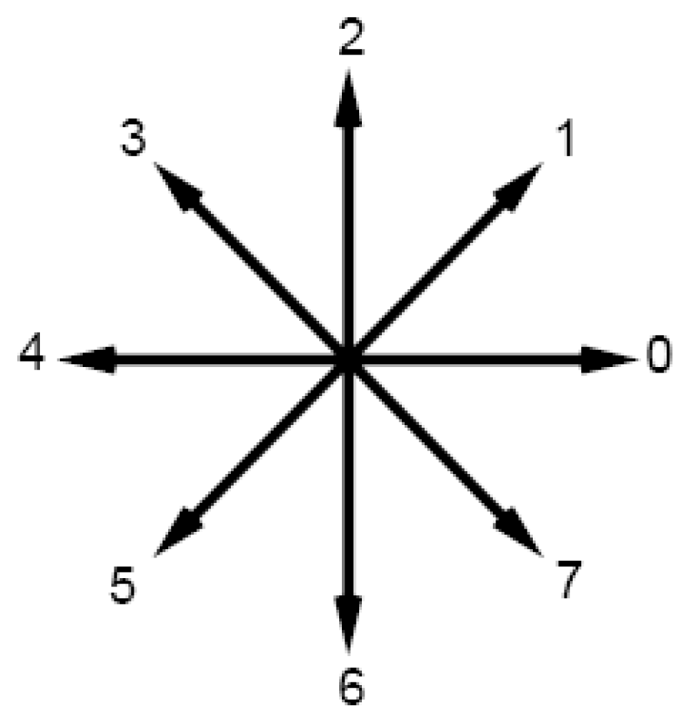
12]. Once line thinning stage is performed, the second stage is line following and chain coding the medial axis. In this stage, tracing process starts at an end pixel and continues based on the chain code directions until the last pixel in the line is reached.
Fig-1 indicates the eight possible directions specified by the numbers from 0 to 7. Detail information on chain coding process can be found in [
13 -
14 -
15]. At the third stage, the medial axis coded in the second stage is examined and the vectors in the chain code are identified. In this process, the long vectors that closely represent the chain codes are formed while considering a user defined maximum deviation of the vectors from the chain codes [
16 -
21].
In this study, a new model, MUSCLE (Multidirectional Scanning for Line Extraction), was developed to vectorize the straight lines through the raster images including township plans, maps, architectural drawings, and machine plans. Unlike traditional vectorization process, this model generates straight lines based on a line thinning algorithm, without performing line following-chain coding and vector reduction stages [
22].
2. Material and Method
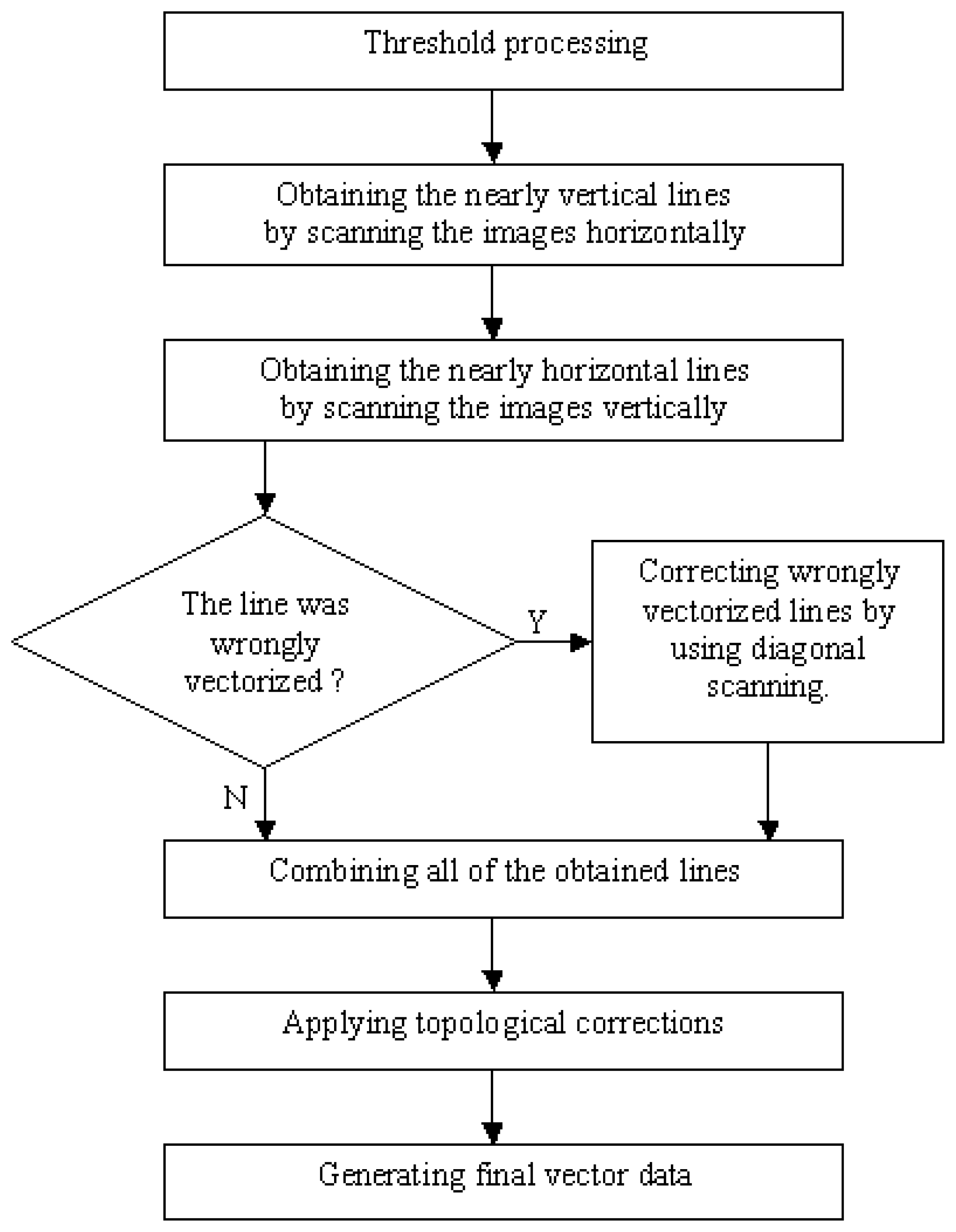
The logic behind the model is presented in
Fig-2. The following main stages in the model are described in this section:
Threshold processing
Horizontal and vertical scanning of the binary image
Detecting wrongly vectorized lines
Correcting wrongly vectorized lines by using diagonal scanning
Applying topological corrections
Generating final vector data
2.1. Threshold Processing
In grayscale images, the objects may contain many different levels of gray tones. In this study, the objects are separated by using the threshold processing technique, with the assumption that the gray values are distributed over the image nearly homogeneous [
17 -
18 -
19]. In the threshold process, a predetermined gray level (threshold value) is to be determined and every pixel darker than this level is assigned black, while every lighter pixel is assigned white. Therefore, the grayscale image was converted into a binary image [
20 -
21].
2.2. Horizontal and Vertical Scanning of the Binary Image
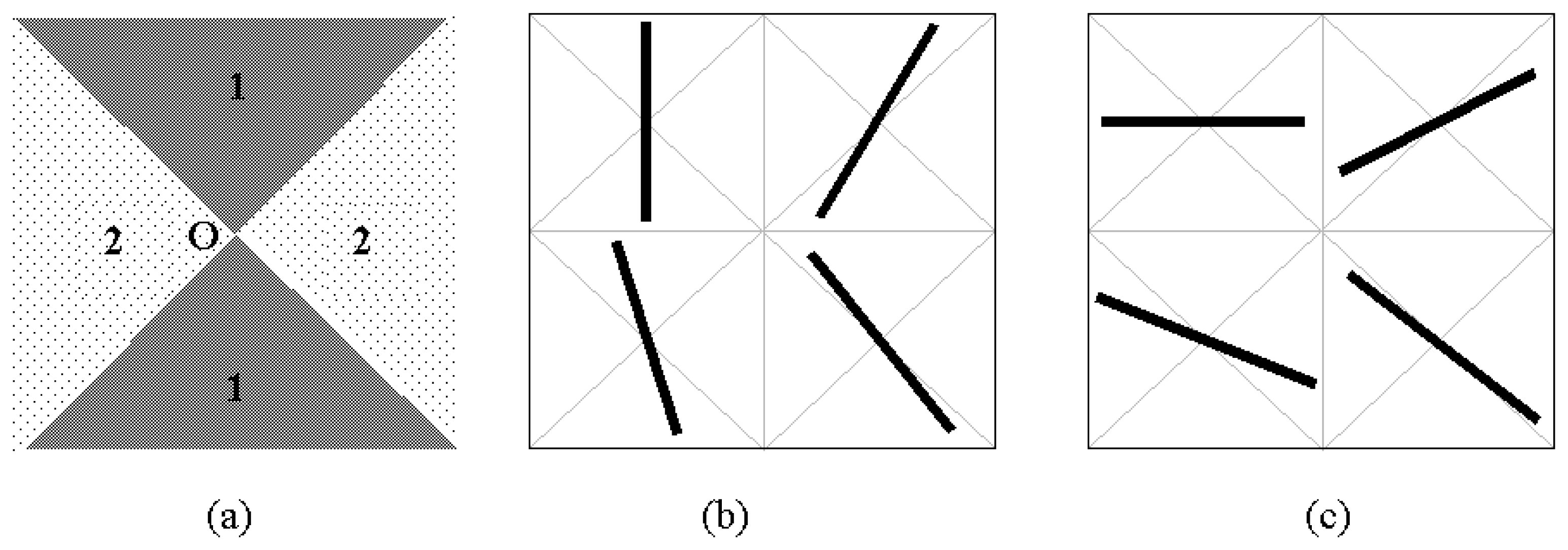
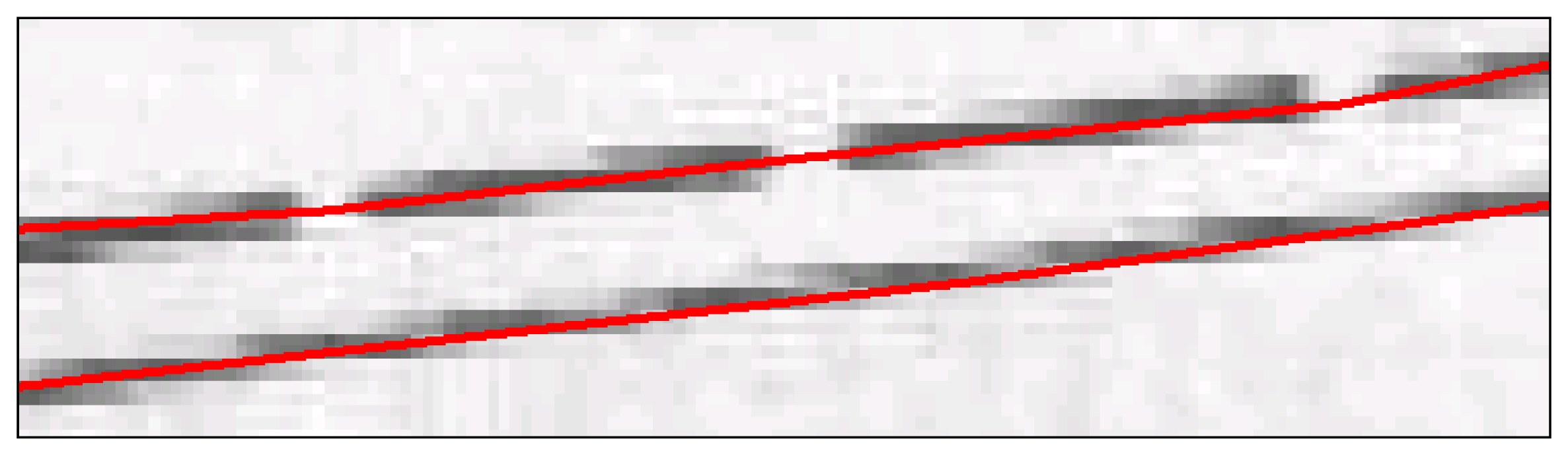
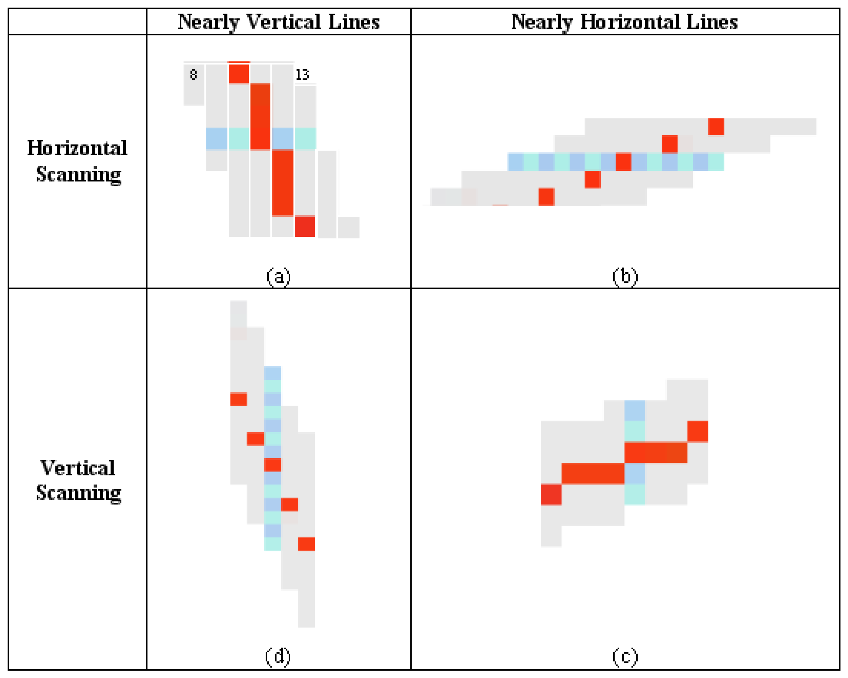
In this stage, the horizontal and vertical lines were extracted from the binary image. The nearly vertical lines were obtained by scanning the images horizontally, while the nearly horizontal lines were obtained by scanning the images vertically. The forms of nearly vertical and nearly horizontal lines are shown in
Fig-3. In
Fig-3a, the lines which pass through the region 1 and 2 are defined as the nearly vertical lines and the nearly horizontal lines, respectively.
Fig-3b and Fig-3c indicate the sample drawings for nearly vertical and nearly horizontal lines, respectively. In other words, if the slope (tangent) of the line is between -1 and +1, it is defined as “nearly horizontal line”. If the slope (tangent) of the line is less than -1 or greater than +1, it is defined as “nearly vertical line”.
At the first step, each row on the binary image was scanned horizontally to determine the thickness of the lines and the position of the pixels, which were located in the mid-point of the lines. During this process, the value (black or white) of each pixel was checked by moving from left to right. Once the first black pixel was met, its column number was stored into the algorithm. While continuing to scan pixels, the column number of the first white pixel was also stored into the algorithm. Thus, the position of the middle pixel in the mid-point of the line could be determined by using the following equation, based on the image coordinate system:
| m | : column number of the first black pixel |
| n | : column number of the first white pixel |
For example, assuming that 8
th pixel is the first black pixel and 13
th pixel is the first white pixel in
Fig-4a. Using
Equation 1, position of the middle pixel can be calculated as 10
th pixel, which is then colored with red. After performing the same process for each row on the image, distribution of the red pixels for nearly vertical and nearly horizontal lines is indicated in
Fig-4a and Fig-4b, respectively. In these Figures, the distribution of the red pixels indicates that the red pixels have continuity for nearly vertical lines; however they have discontinuity for nearly horizontal lines.
After the horizontal scanning processes were completed, only the red pixels were selected. Then, a neighborhood analysis was carried out based on the nearly vertical lines by taking the advantages of discontinuity on the nearly horizontal lines. In this method, a red pixel, which is adjacent to another red one, was searched along the lines. This process continued until no red pixels were found adjacent to each other, indicating that the end of the line has been reached. The beginning and ending points of all the nearly vertical lines were determined by using the same procedure.
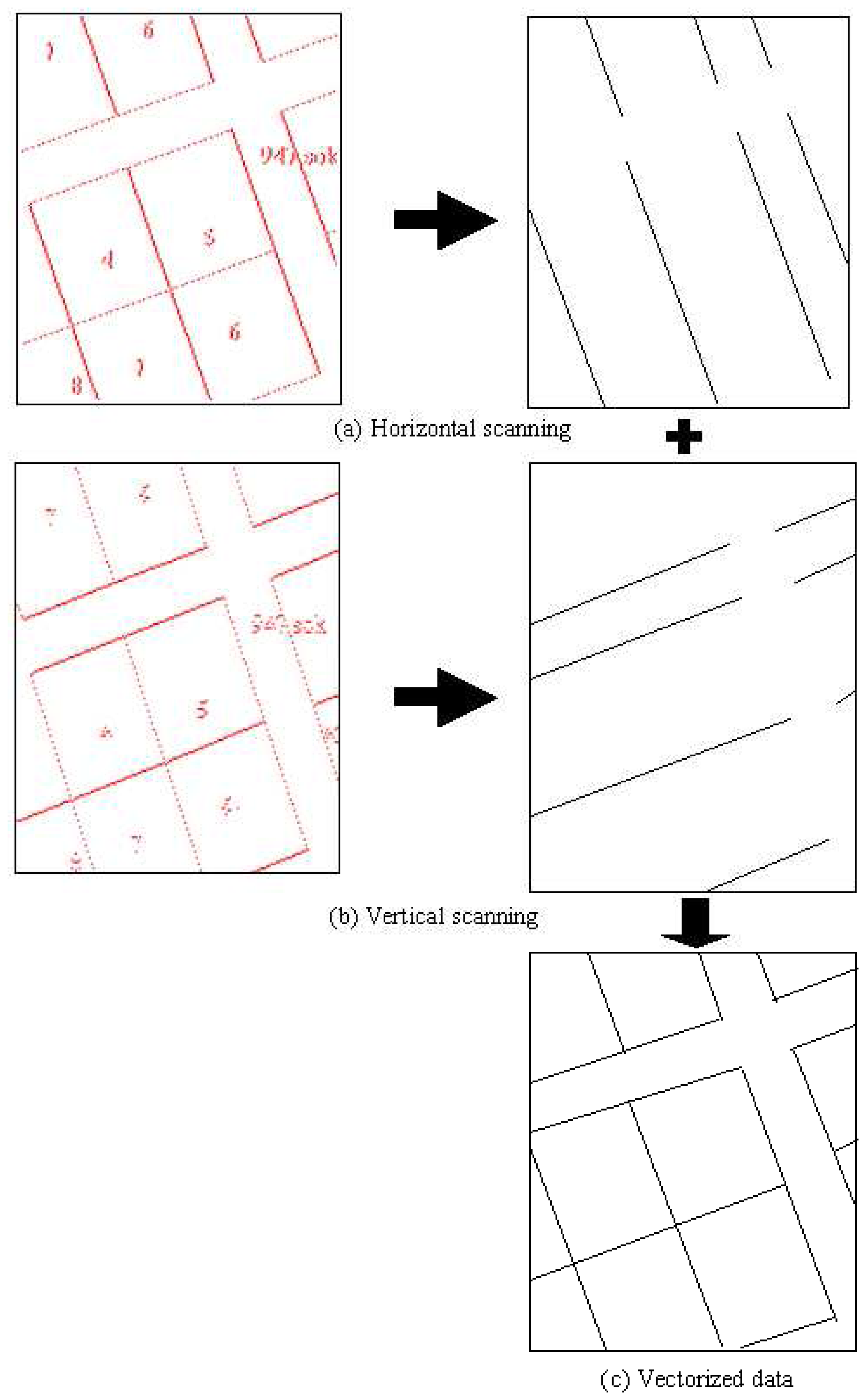
At the second step, the binary image was scanned vertically, and then, the same process described above was carried out for all columns. Unlike horizontal scanning, the red pixels have continuity for nearly horizontal lines (
Fig-4c); however they have discontinuity for nearly vertical lines (
Fig-4d). Therefore, the neighborhood analysis was carried out based on the nearly horizontal lines and the beginning and the ending points of all the plenary horizontal lines were determined. After completing the horizontal (
Fig-5a) and vertical (
Fig-5b) scanning of the binary image, the final vectorized data (
Fig-5c) were generated by vectorizing the nearly vertical and the horizontal lines.
2.3. Detecting Wrongly Vectorized Lines
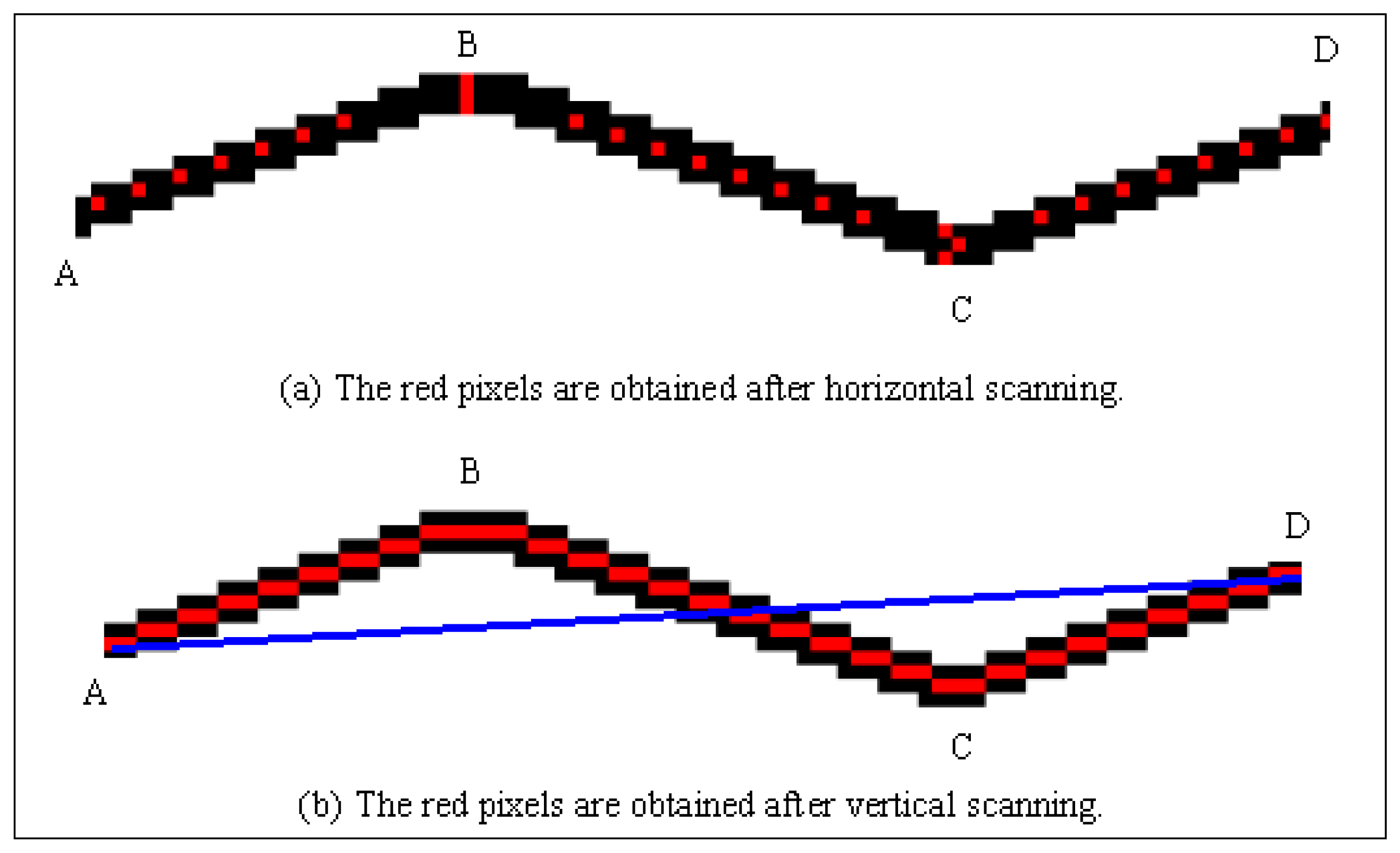
In a case where two or more consecutive lines are nearly horizontal or nearly vertical, raster data become unmanageable and the process described in the previous stages generates wrongly vectorized lines. For example, initially, three consecutive nearly horizontal lines (AB, BC, and CD) were horizontally scanned as displayed in
Fig-6a. Due to discontinuity of the red pixels between intersection points A, B, C, and D, the neighborhood analysis cannot be performed and vectorized data cannot be generated. When the raster image was vertically scanned during the second step, the neighborhood analysis yielded wrong vectorization results because of continuity of the red pixels. The algorithm recognizes point A as the beginning point of the line, skips point B and point C, and ends the line at point D. Therefore, the process generates a wrongly vectorized line between points A and D as indicated in
Fig-6b.
The detection of wrongly vectorized data is performed by comparing the middle axis of the lines (red pixels) with the vectorized lines. The middle axis and the vectorized line have to be based on the same linear equation. For example, if a sample vectorized line (AB line) is a line with the beginning point of A(
xa,
ya) and the ending point of B(
xb,
yb), then, the linear equation for this vectorized line can be formed as follows:
When
X coordinate of a red pixel is inserted into the linear
Equation 3, and if the difference between the
Y value derived from this equation and the
Y coordinate of this pixel is greater than a user defined maximum deviation, the model defines this line as a wrongly vectorized line. After this process, the red pixels within the acceptable deviation range were eliminated from the image by converting them into the white pixel values. The wrongly vectorized lines with red pixels were remained unchanged within the image.
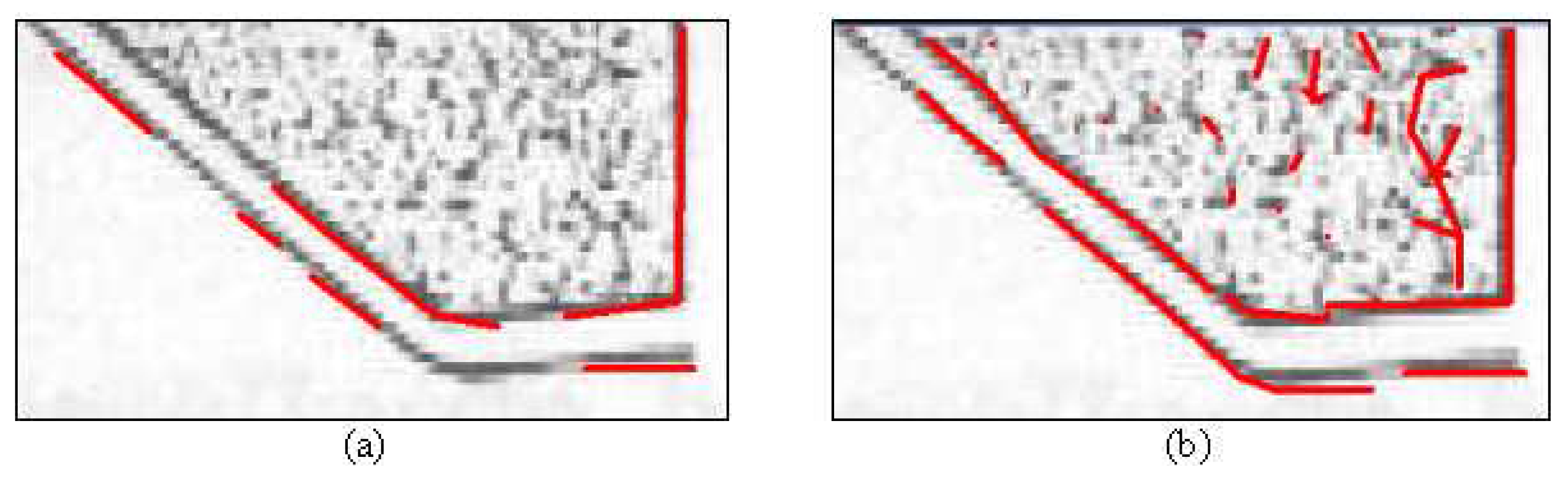
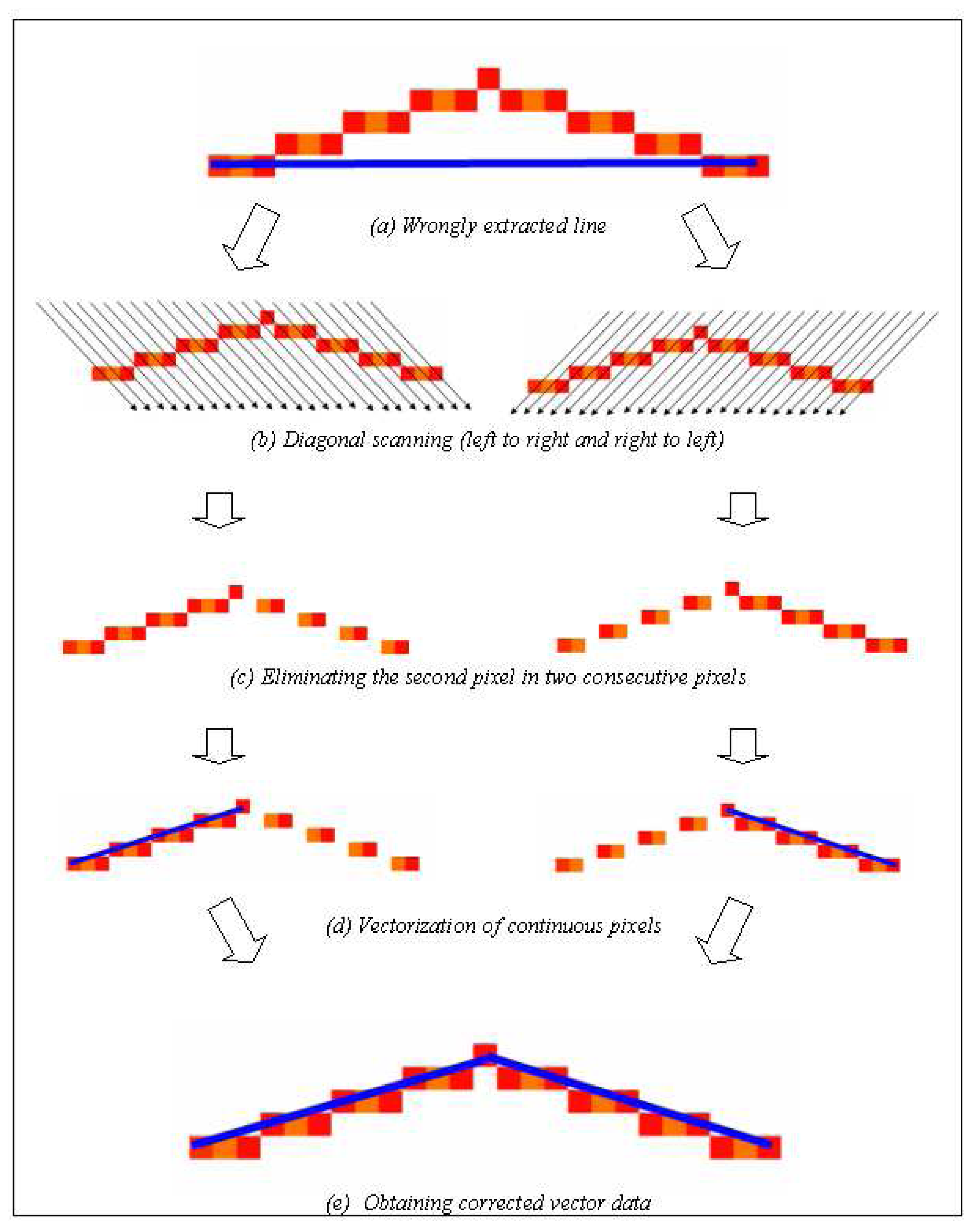
2.4. Correction of wrongly vectorized lines by using diagonal scanning
The image with the wrongly vectorized lines (
Fig-7a) was diagonally (under 45
0 angle) scanned; first, from left to right, and then, from right to left (
Fig-7b). In diagonal scanning process, if there were two consecutive red pixels along the direction of scanning, the second red pixel is eliminated. Thus, vectorized line took a discontinuous form as shown in
Fig-7c. After applying the neighborhood analysis, the lines failed to have the acceptable number of pixels were not vectorized. The continuous pixels, determined by implementing diagonal scanning from both directions, were vectorized as indicated in
Fig-7d. Then, corrected vector data were generated by combining both of the vectorized lines together (
Fig-7e).
2.5. Applying Topological Corrections
Once horizontal, vertical, and diagonal scanning processes were completed, the topological corrections for the intersection points of the lines should have been performed. Topological corrections are very important to efficiently use the extracted vector data in GIS and other spatial applications.
2.5.1. Connecting End Points of the Lines
This circumstance occurs especially at the corner points. The correction was performed by using a special criterion as explained in the following section. This criterion was based on selecting a user-determined distance between the lines. The adjacent lines in the selected distance were connected at the algorithm. Then, the end points are joined by calculating the mean value of coordinates for two or more nodes as follows (
Fig-8):
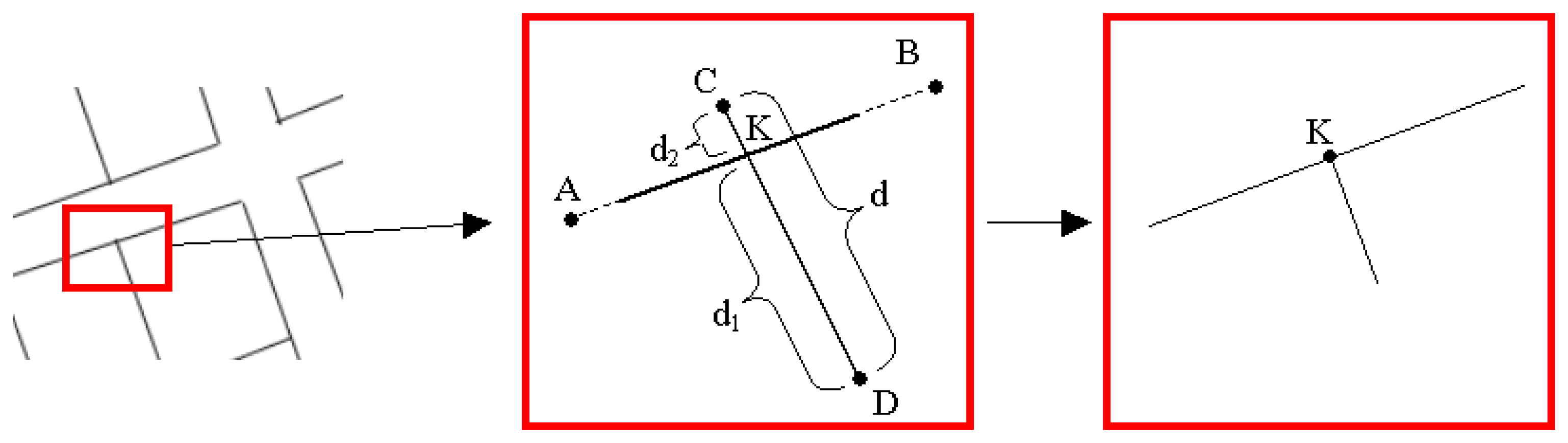
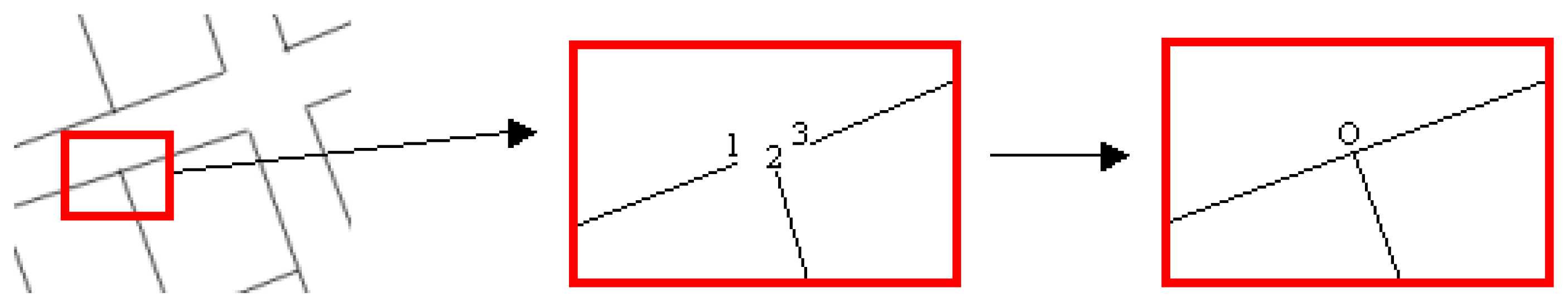
2.5.2. Correction of Overshoot and Undershoot Errors
In this process, firstly; the coordinates of the intersection points between the lines were calculated as follows (
Fig. 9):
Secondly, point
A(xa,ya) and point
B(xb,yb) were used to determine the beginning and ending points of the line. The other line can be defined by point
C(xc,yc) and point
D(xd,yd) as follows:
Then, the coordinates of the intersection point (
K) for these two lines can be calculated by the formulations in
Equations 8 and
9, respectively:
The distances (
dn) from an intersection point,
K(xk,
yk), to the ending points of the intersecting lines can be calculated by using the following equation:
After determining the coordinates of the intersection point and the distance between intersection point and the ending points, ending points were examined to determine either there were overshoot or undershoot errors. If the length of a line (
d) was equal to sum of the distances from two ending points (
d1 and
d2) to intersection point (
K) and one of these distances was shorter than a user defined distance value (
p: explained in Section 2.7.6), ending point was defined as overshoot (
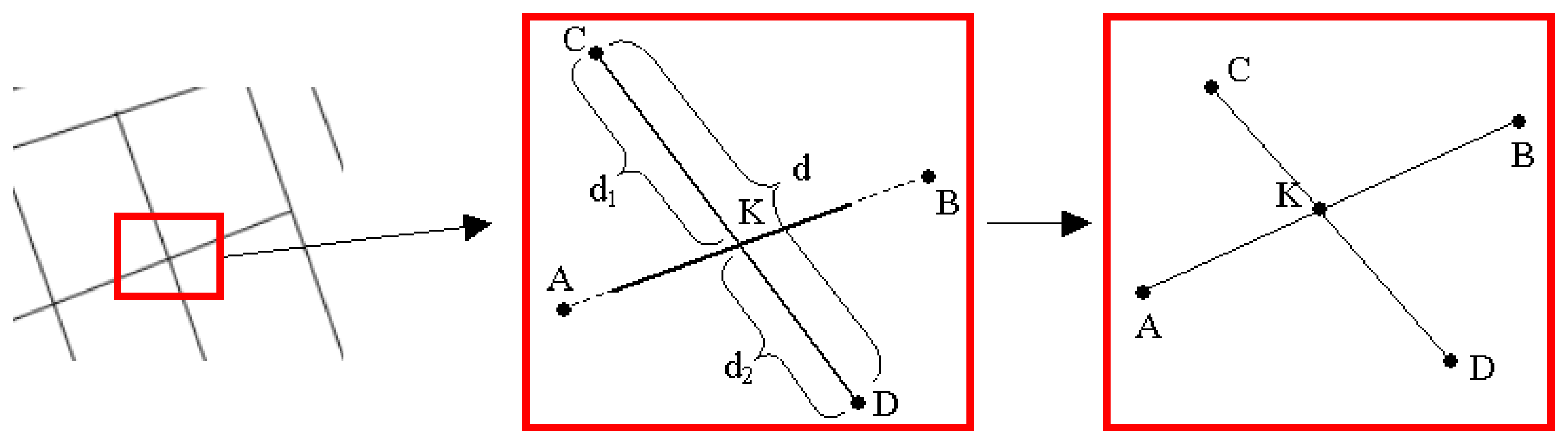
Fig. 9). If the length of a line (
d) was shorter than the sum of the distances from two ending points to intersection point and one of these distances was shorter than a user defined distance value (
p), ending point was defined as undershoot (
Fig. 10). Then, the algorithm corrects the overshoot and undershoot errors by moving the ending point to the intersection point.
If there is a case where the length of a line (
d) was equal to sum of the distances from two ending points to intersection point and both of these distances were longer than a user defined distance value (
p), ending point was not defined as neither overshoot or undershoot. In this case, intersection point is assigned to be a new point and the lines were divided into four new lines as indicated in
Fig. 11.
2.6. Generating the Final Vector Data
The product obtained after the vectorization process is saved to be ready to use in the “DXF” format, which is the “de facto” standard and well known exchange CAD format by all CAD software. Each output images generated after scanning and correction stages can be recorded as separate layers; therefore, the user can monitor the vectorization process and use these layers for various purposes.
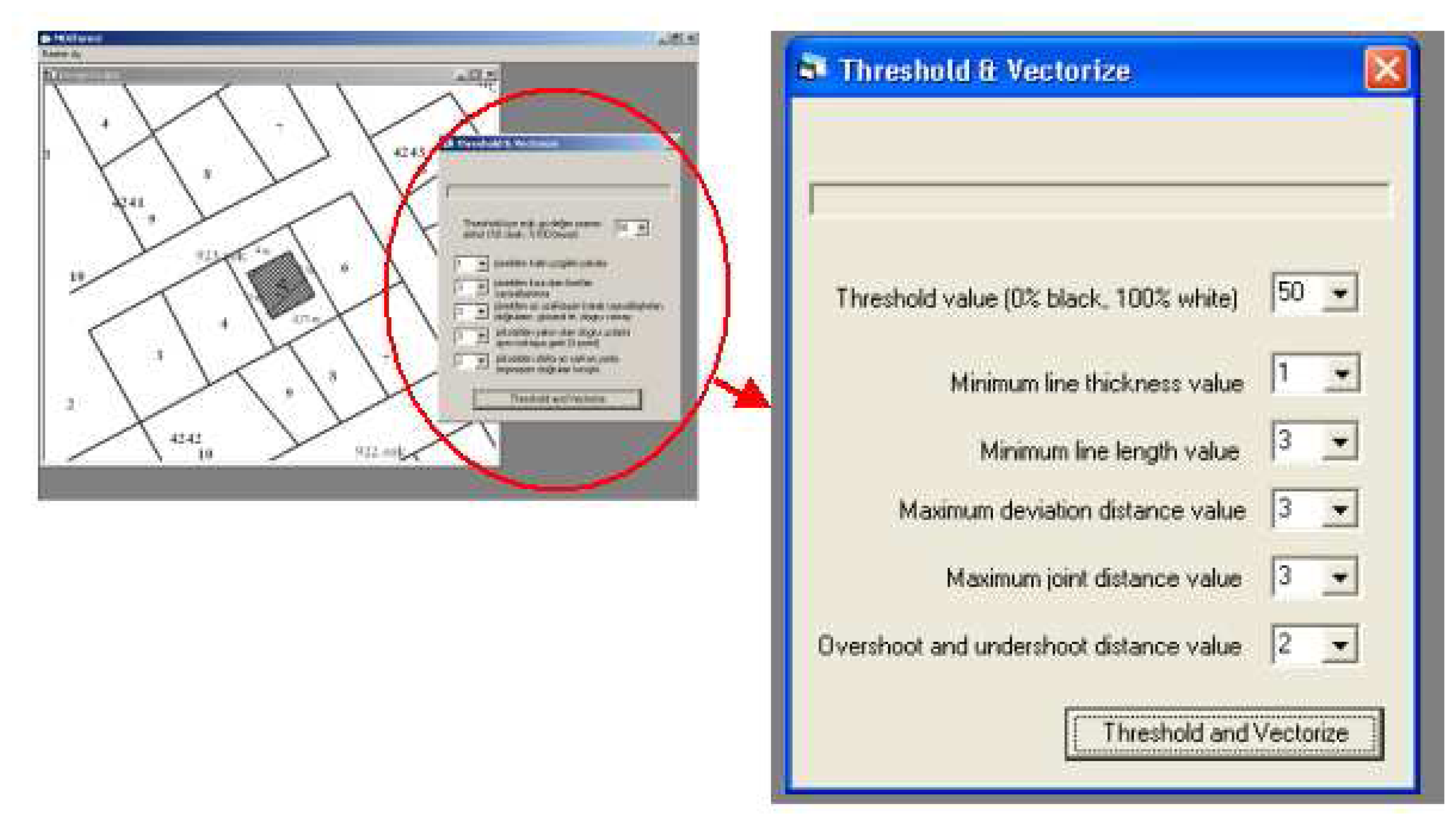
2.7. Graphical User Interface and the Criteria
The algorithm was programmed in Visual Basic 6.0 platform and the graphical user interface of the model is displayed in
Fig-12. The user is expected to define the specified criteria for the current raster and the future vector data before the vectorization process. The performance of the vectorization depends remarkably on these six criteria.
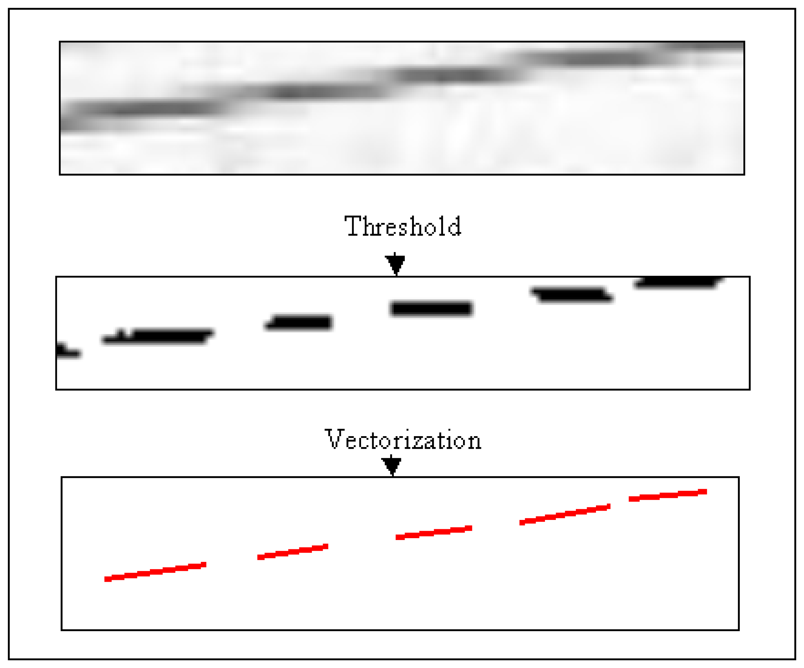
2.7.1. Threshold Value
Threshold value was used to define two main classes, black and white, based on the gray value distribution of the raster image. Gray values under the threshold value become black, while values above the threshold become white. Depending on the threshold value, some lines can be thicker and clarified, while some lines can be thinner and fader. Therefore, selecting an optimum value for the threshold according to the raster properties is very important for the success of the vectorization process. This optimum value can be found after having some experiences based on the trial. For example, by looking at the darkness of the output image, user can come up with optimum threshold value.
2.7.2. Minimum Line Thickness
The second criterion was the thickness of the lines in the raster image to be vectorized. For example, if the user selects three as a minimum number of pixels for line thickness, lines thinner than three pixels are ignored and not vectorized. This is useful when the user wants to extract certain objects like parcel boundaries with certain line thicknesses.
2.7.3. Minimum Line Length
Another criterion for eliminating the unnecessary details and for vectorizing the lines with sufficient length was the assignment of the minimum number of the pixels for the line length. For example, if a user selects six for this criterion, the algorithm eliminates lines that are shorter than six pixels during the vectorization process. Thus, unwanted objects such as text and noise can be eliminated from the raster image much more easily.
2.7.4. Maximum Deviation Distance
The determination of the wrongly vectorized lines was performed by considering the deviation distance between the red pixels and the vectorized line as described in section 2.3. The maximum deviation distance is defined by the user based on the sensitivity of the job. For instance, if a user selects three for this value, the vectorized lines that are more than three pixels away from the red pixels would be considered to be in the incorrect form, whereas the lines that are closer than this value would be considered to be in the correct form.
2.7.5. Maximum Joint Distance
During the topological correction of the vectorized data, the ending points of the lines that were closer to each other must have been merged for joining the broken lines. For achieving this, the user is allowed to define and input a maximum joint distance value. Consequently, if the distance between ending points of the lines is less than the input value, the model connects these points at a shared intersection point.
2.7.6. Overshoot and Undershoot Distance
The user is allowed to define and input a distance value for correcting the undershoot and overshoot errors during the vectorization process. For example, if a user assigns the value of three for this criterion, dangles and gaps which are smaller than three pixels would be eliminated and geometrically corrected as explained in section 2.5.
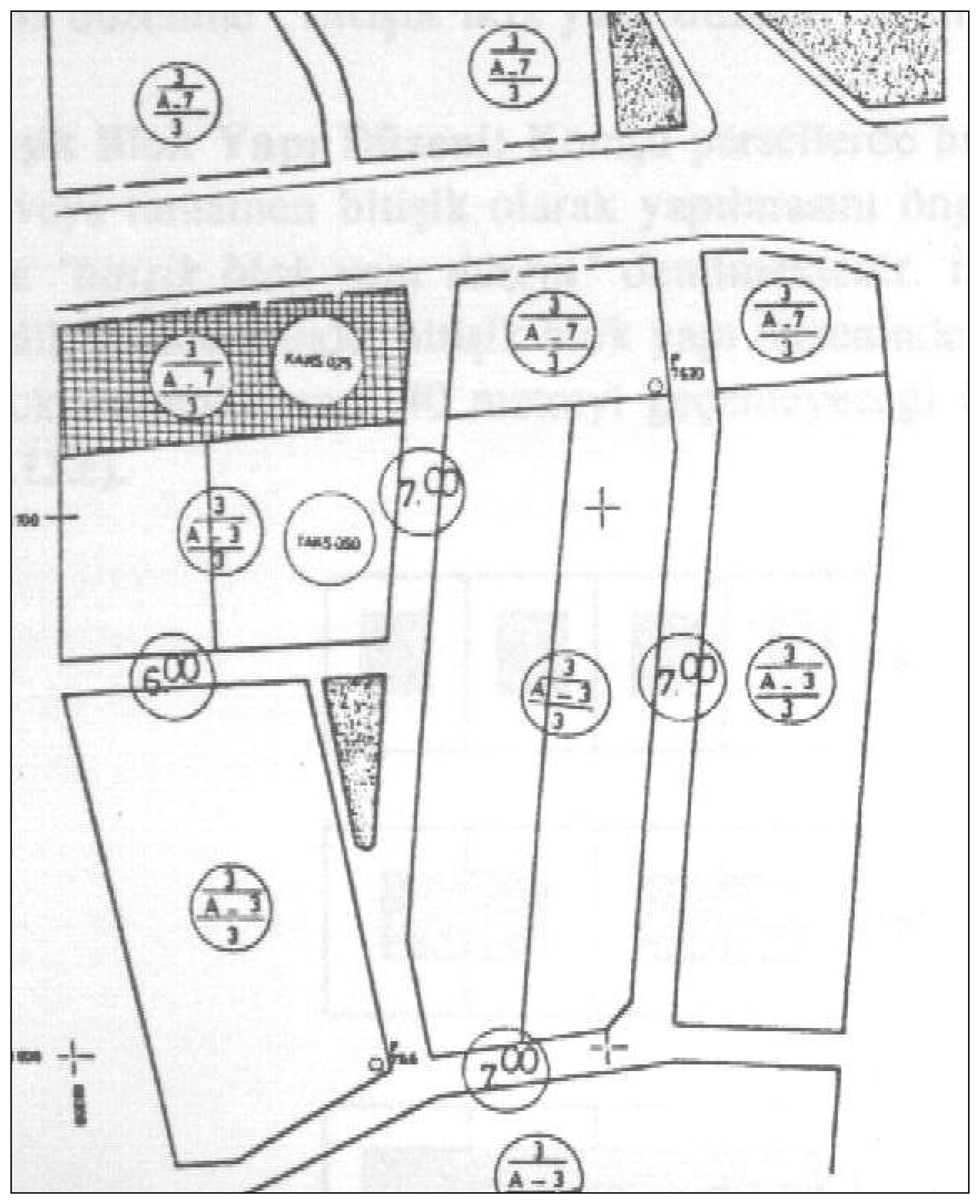
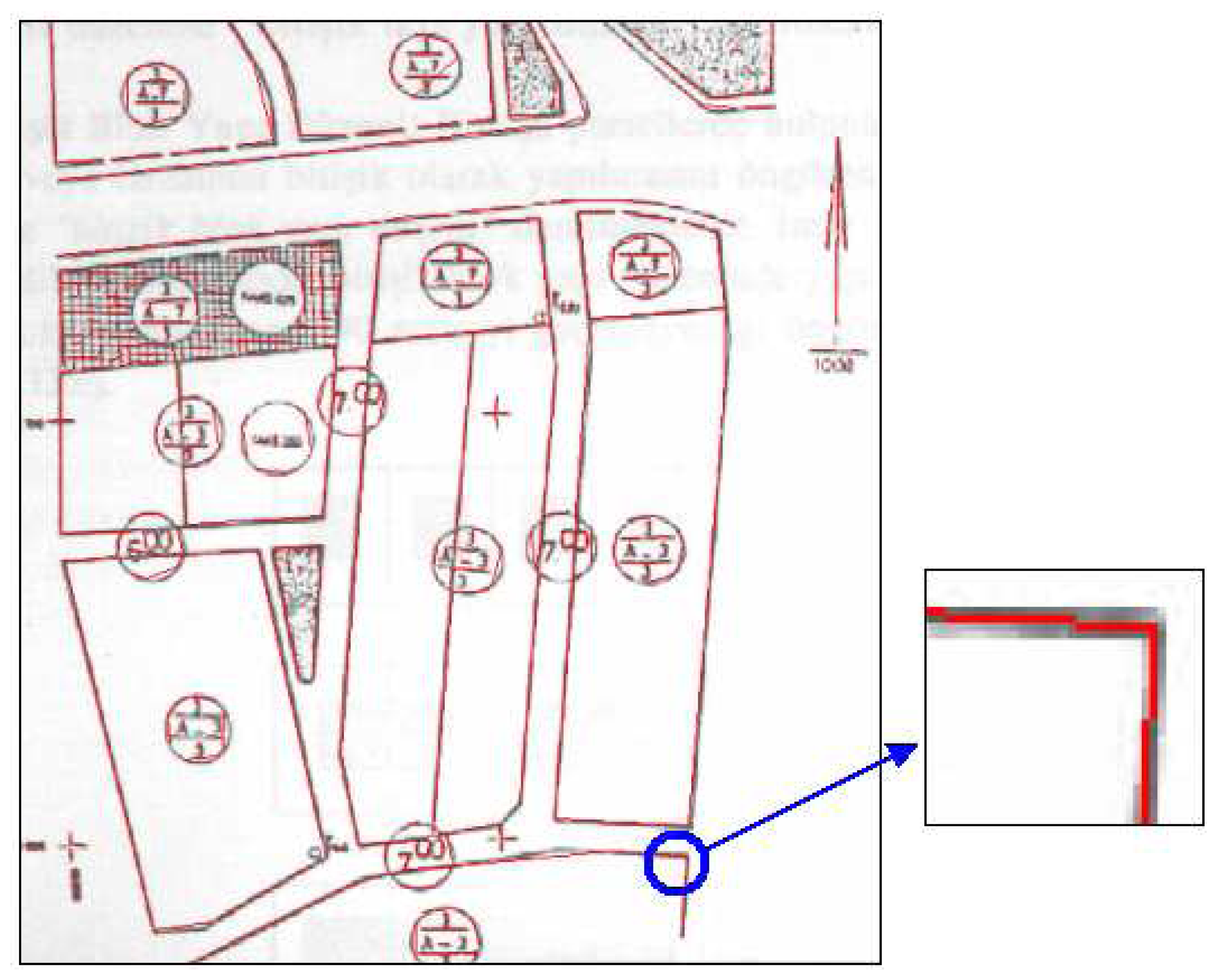
3. Results and Discussion
The algorithm was tested on a sample raster data of a township plan. In Turkey, township plans are highly desired maps which are generally in analogue format and subject to intensive digitizing tasks. In the model application, vectorization algorithm was applied on the map exposed in
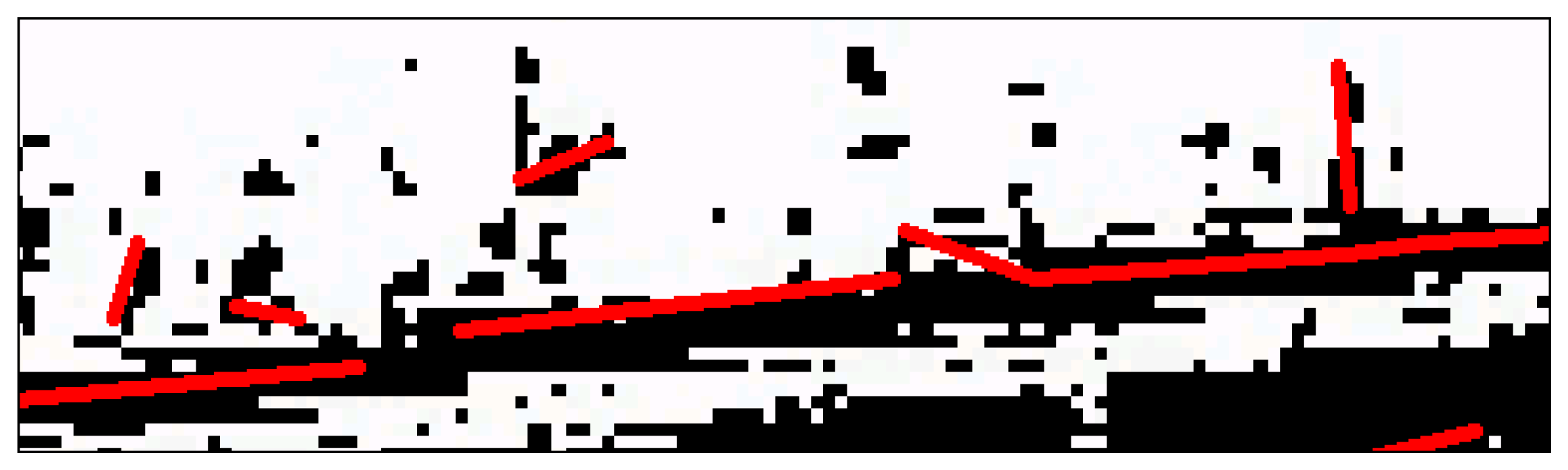
Fig-13The user-defined values were assigned to the criteria described in the previous section. Setting a low threshold value (50%) caused discontinuity along the lines during vectorization processes (
Fig-14). However, setting a high threshold value (90%) resulted in very thick lines with noises; therefore, it caused the algorithm to induce errors and yielded bad results (
Fig-15).
If the thickness value of the line was selected to be very big, some of the necessary lines were ignored in the process (
Fig-16). For example, when the minimum number of pixel for the line thickness was decreased, the one pixel- thickness was ignored in the vectorization process.
For the third criterion, when the number of pixels for the minimum line length was selected as a very big value (e.g. 9 pixels), the noise problem was mostly solved, however, some of the lines along the parcel boundaries were failed to be extracted (
Fig-17a). On the other hand, when the value of this criterion was set to be a low value (e.g. 3 pixels), almost all of the lines along the parcel boundaries were extracted. However, it was observed that some of the noises over the lines were also vectorized (
Fig-17b).
If the value of the fourth criterion, the deviation distance between red pixels and the vectorized line, was selected to be a high value, the chance of ignoring the lines that were wrongly vectorized tends to increase (
Fig-18). When the fifth criterion was selected to be a high value, the lines that were not intended to be processed were merged and vectorized as seen in
Fig-19. The model application also revealed that setting a low value for the sixth criterion had yielded better results regarding the correction of the overshoot and undershoot errors.
In order to generate the best vectorization out of the sample data, a number of alternative values were tested over the criteria. The goal was to vectorize all the lines at the parcel boundaries and to eliminate the remnants of the noises and texts as mush as possible. Our results indicated that the best vectorization was performed by using the following combinations over the criteria:
The threshold value as 65%,
The minimum line thickness value as 1 pixels,
The minimum line length value as 6 pixels,
The maximum deviation distance value as 4 pixels,
The maximum joint distance value as 4 pixels,
The overshoot and undershoot distance value as 2 pixels.
The final vector data generated by applying the vectorization process with the criteria above are displayed in
Fig-20. Consequently, a great success was achieved for fixing the lines at the parcel boundaries; however, the noises could not be removed completely.
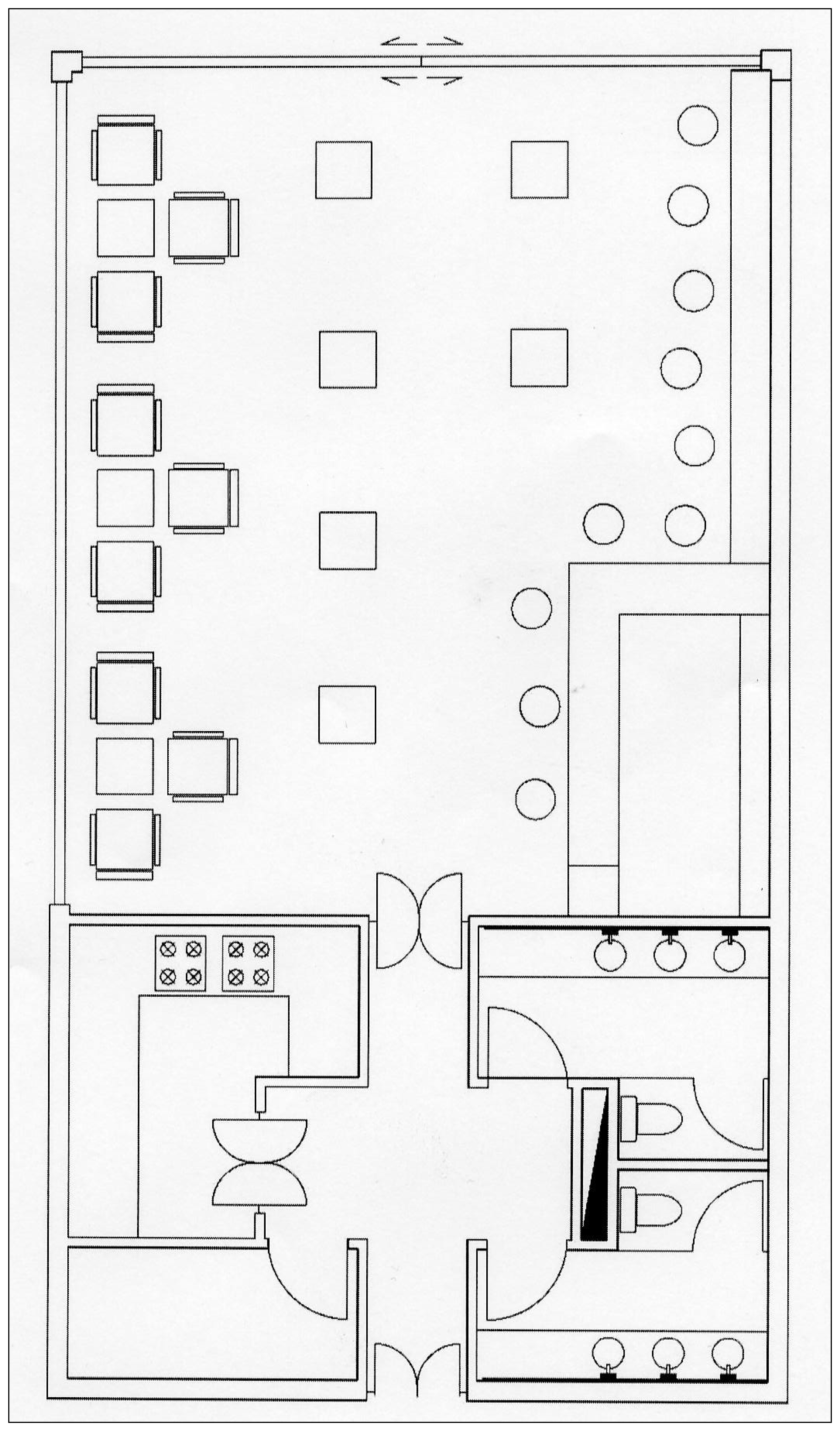
The performance of the proposed model was evaluated by comparing the results with two commercial raster-to-vector programs, WinTopo and Scan2CAD. For comparison, the images in
Fig. 13,
Fig. 21, and
Fig. 22 were processed by all the three models and the results were indicated in
Table 1. The images were acquired in 200 dpi and 8 bit radiometric resolution by using scanner. So, before the threshold processing, images have 256 grey values.
Our results indicated that WinTopo completed the vectorization process in the shortest computation time; however, it divided the lines into many pieces, which resulted in too many objects. This also required intense and time consuming post-processing process after the vectorization. Scan2CAD performed a quality vectorization process with acceptable number of objects. However, there were still some errors on vector images.
MUSCLE also provided very successful results, especially for the images with straight lines. The model generated an individual vector for each piece of line, which reduced the number of final objects. This feature also reduced the computation time in the process of correcting the errors. However, total time spent on vectorization process was longer than the time spent by using the other two commercial programs since the current version of the MUSCLE was not professionally optimized.
5. Conclusions
In this study, a new model, MUSCLE, was developed by implementing an appropriate computer programming to automatically vectorize the raster data with straight lines. The model allows users to define specified criteria which are crucial for the success of vectorization process. A basic vectorization application presented in this study cannot be totally generalized, yet it showed that this model is able to successfully vectorize raster images with straight lines. More work in necessary to improve the quality of the vectorized image such as automated selection of user defined optimum combinations for the criteria.
The unique contribution of this model can be described briefly as its potential for vectorizing straight lines based on a line thinning and simple neighborhood analysis, without performing line following-chain coding and vector reduction stages. Besides, the model has the ability to vectorize not only the maps with linear lines such as cadastral map sheets, township plans, etc., but also other documents such as technical drawings, machine pieces, architectural drawings, etc., which are to be converted from a analogue format to digital format. It is highly anticipated that MUSCLE can provide a quick and simple way to efficiently vectorize raster images. There are several opportunities to improve this model such as vectorizing curve lines and refining model interface.
The sample application, where the performance of the model has been compared with the two well known commercial vectorization programs, indicated that the current version of MUSCLE can perform a successful vectorization task. It was believed that refining and optimizing the algorithm by professionals would improve the vectorization process. Further researches are also required through an extended and a diversified sample space to expose the feasible application areas of MUSCLE. Yet, our results suggest that MUSCLE may offer opportunities for replacing the complicated digitizing tasks with a concise, automatic and computer-aided process.


