1. Introduction
A participatory sensing system [
1] supports a large number of mobile users to collect sensor data and share the information of their environment. Many sensor data and mobile services are location oriented. For example, a driver may want to know the gas price of nearby gas stations or the traffic conditions around a specific area. Potential applications of location-based services in participatory sensing range from personal healthcare, object search to entertainment. However, obtaining location information often requires large energy consumption, which may discourage many mobile participants. Given the limited battery life of a mobile device, it is crucial to minimize the energy consumption in localization.
GPS localization is known as a major source of energy consumption in mobile devices. Continuous GPS sensing can easily drain the battery of a mobile device in five to six hours [
2]. However, many participatory sensing applications require the mobile devices to turn on their GPS to collect location information. Even though alternative localization methods are available, such as cell-tower-based localization and WiFi-based localization, they fail to provide the same level of accuracy as the GPS.
The traditional approach consumes much energy, as each mobile device has to turn on its GPS continuously to collect and report sensor and location data to the server. To address this problem, we propose a novel approach of collaborative localization, which suggests that mobile devices share location information with other devices in the same vicinity. Apart from sharing GPS readings, we leverage lightweight sensors, such as the accelerometer and gyroscope, to approximate the location of individual devices in collaborative localization. These lightweight sensors can run for more than 20 h continuously on a smartphone [
3], which can assist localization and reduce energy consumption.
Different from the traditional approach, our proposed approach divides the mobile devices into three categories, the broadcasters, the location information receivers (LIRs) and the normal participants. All members in the three categories collect sensor data periodically, but the ways that they obtain location data and label sensor data are different. The broadcasters and the normal participants turn on their GPS to obtain their location data, which are then used to label their sensor data. To save energy, the LIRs do not turn on their GPS. Instead, they estimate their locations according to the location information broadcast by the surrounding broadcasters.
Each mobile device will be assigned to a category by the server, and its category will be updated from time to time. We formulate the broadcaster set selection problem (BSSP) to select the set of broadcasters and to determine how long the selected mobile devices will be broadcasters. The LIRs will use the location data from the broadcasters nearby to estimate their own locations. The remaining stand-alone mobile participants are the normal participants, who use GPS to obtain location data as in the traditional approach. The objective of BSSP is to minimize the overall energy consumption of all of the participants.
The contributions of this paper are summarized as follows:
A collaborative localization architecture is proposed, which enables flexible adjustment on location accuracy based on the application requirement. A mathematical model is set up to measure the total energy consumption of mobile participants.
The operations in collaborative localization are designed and presented, which are feasible to be implemented for participatory sensing systems.
The BSSP is formulated, which aims to minimize the energy consumption of all of the participants.
Two novel heuristic algorithms are proposed to solve the BSSP.
The performance of the proposed solution has been evaluated thoroughly by simulations using real mobility traces. The results show that our proposed algorithms can save up to 68% of the total energy in localization.
A preliminary conference paper based on this work can be found in [
4]. The rest of the paper is organized as follows.
Section 2 presents the related work.
Section 3 shows the system architecture and information flows.
Section 4 shows the energy model and formulates the BSSP.
Section 5 describes our proposed broadcaster set selection algorithms.
Section 6 evaluates the performance of our proposed algorithms by simulations using real mobility traces. Finally,
Section 7 concludes the paper.
2. Related Work
There are several types of mobile sensing, including participatory sensing, opportunistic sensing and crowdsensing [
5]. The key idea of mobile sensing systems [
5] is to have ordinary citizens collect and share sensor data from their surrounding environment by using their smartphones. For example, the Common Sense project [
6] has developed a participatory sensing system that allows mobile participants to measure their personal exposure to air pollution. Similarly, Kanjo [
7] has shown a system that allows participants to collect and share the noise pollution information. Zhang [
8]
et al. have proposed a new cosine theorem-based method for identifying and expressing conflicting data, which can be used for fusing conflicting data collected by participants.
In addition, research work has been done to address the participant selection problem in mobile sensing. Tuncay
et al. [
9] have exploited the user behaviors and selected the participants based on their mobility history. However, this approach relies heavily on the knowledge of participant trajectories, which increases the risk of leaking user privacy. Reddy
et al. [
10] have developed a selection framework that enables organizers to choose well-suited participants to collect data. Similarly, Song
et al. [
11] have developed a participant selection framework to satisfy the quality-of-information (QoI) requirements of the sensing tasks. Other than that, Lu
et al. [
12] have studied initiating sampling around a specific location. However, all of the above schemes could be further improved by taking energy saving into consideration.
Energy saving is a very important issue in mobile sensing systems. One common approach is to reduce the sampling rates, though this may lead to lower accuracy of the sensing results [
13,
14]. Other approaches utilize additional sensors, such as accelerometers and orientation sensors, to assist localization [
15]. However, none of the above works have explored the possibility of sharing location information with neighboring devices.
Different from the traditional approach using GPS, alternative localization methods have been exploited. For example, Johnson and Seeling [
16] have proposed a scheme based on Bluetooth device names to enable power-optimized
ad hoc localization of mobile devices. However, this work mainly focused on the naming scheme, while the optimization of energy consumption during localization remains to be further explored. Other than that, some authors have suggested to use location beacons as localization references [
17], but this method requires either fixed or mobile beacons. Similarly, Zhang and Yu [
18] have proposed a beacon selection method that selects equilateral triangle nodes to be beacons. However, the location beacons may limit the energy saving performance and increase the deployment and maintenance cost.
Different from the above work, we aim to minimize the energy consumption through collaborative localization without deploying any beacon nodes. Besides, we only require users’ current locations instead of any historical trajectories; thus, our approach can protect user privacy.
3. System Architecture and Information Flow
In this section, we first illustrate the system architecture for the participatory sensing system and then describe the information flows of collaborative localization.
3.1. Motivating Scenario for Collaborative Localization
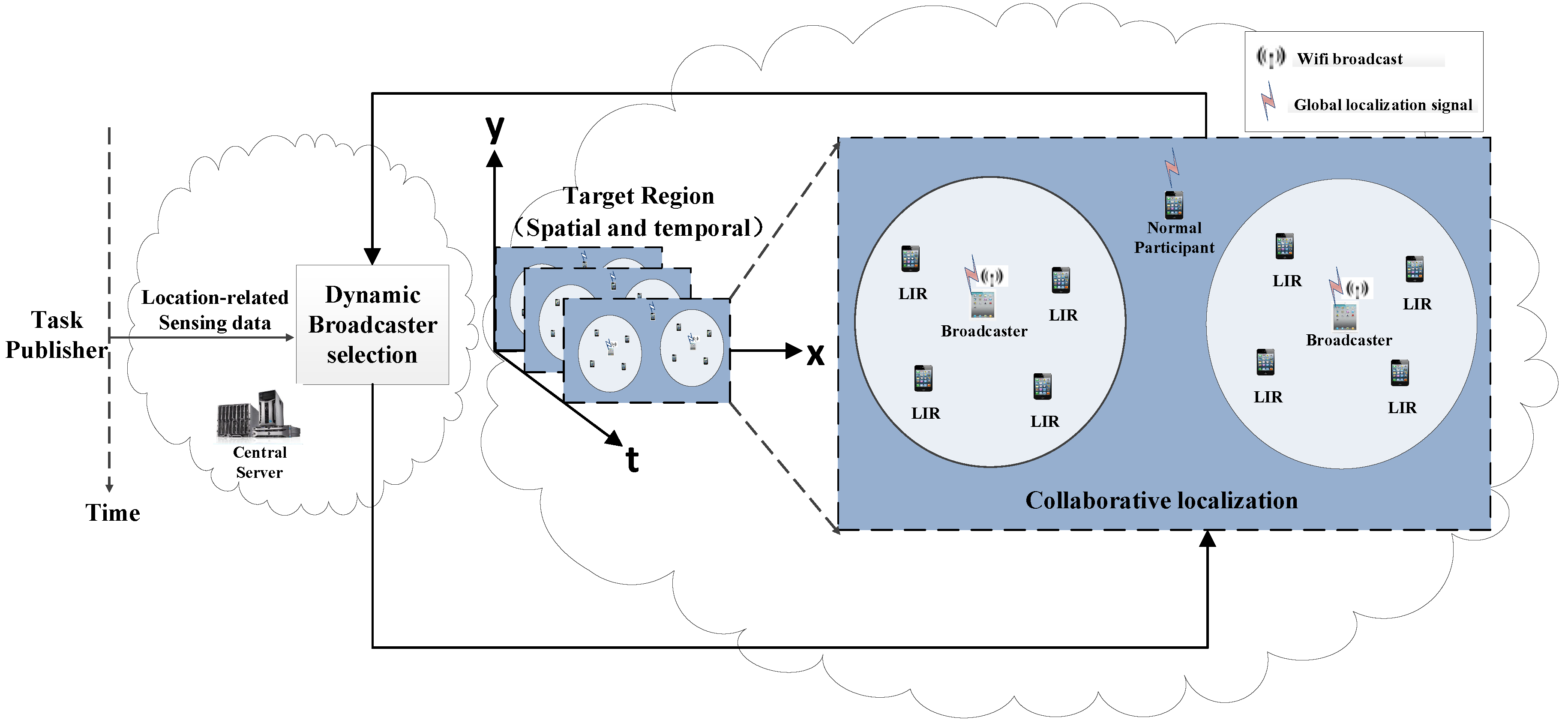
We consider a participatory sensing system in
Figure 1. It consists of a central server, a task publisher and a set of
M smartphone users,
, in the region. The task publisher sends the sensing task to the server. The server then forwards the task to all of the participants.
We divide the length of a sensing task into a set of time slots, denoted by , where and are the start time and the end time of the sensing task. Based on the participants’ current locations, the server will assign different roles to the participants to perform the sensing and localization. The roles will last for a certain period of time, then the server will dynamically assign new roles to the participants based on their updated locations.
All of the participants in our system are divided into three different roles. The first role is the broadcaster, which broadcasts its location and movement information to the surrounding participants. The set of broadcasters during is denoted by , ∈. The second role is the location information receiver (LIR), which relies on the broadcasters’ locations to calculate its own location. The third role is the normal participant, which does not receive any location broadcast from the surrounding. Hence, it has to turn on its GPS to obtain the location. The set of normal participants during is denoted by , ∈.
Table 1 lists the frequently-used notations in the paper.
3.2. Information Flow
After the task publisher publishes the sensing task, the server will send the task to all participants. The participants will register their locations to the server. In the initialization phase, all participants turn on their GPS to obtain their initial locations. Based on the participants’ locations, the server will assign different roles to the participants and how long the roles will last, which is denoted by l.
During each collaborative localization time period, all participants collect sensor data, but they label the location information of the collected data differently. The broadcasters and the normal participants turn on their GPS to obtain their locations. Besides, the broadcasters also broadcast their locations and their movement information periodically to their surrounding LIRs. Based on the received broadcasts, the surrounding LIRs can calculate their locations using the device to device localization method proposed in our previous work [
19]. At the end of the collaborative localization period, all participants upload the collected sensor data and their locations to the server through the cellular network. Based on the participants’ current locations, the server will choose and inform their new roles for the next collaborative localization period and how long this period will last.
Figure 2 shows the collaborative localization during [
]. Let
be the time that the participants need for sending data and receiving the roles. During [
], the broadcasters and the normal participants obtain their locations from their GPS, so that they can label the locations of the collected sensor data directly. On the contrary, the LIRs rely on the broadcasters’ locations to calculate their locations and label the sensor data. During [
], all participants upload the collected sensor data and their labeled locations to the server and wait for the server’s reply. Although all participants start sending at the same time, due to jitter or latency, the collected sensor data will arrive in random order on the server side. There is a time window for the server to receive the data. Similarly, there is a time window for the participants to receive the roles.
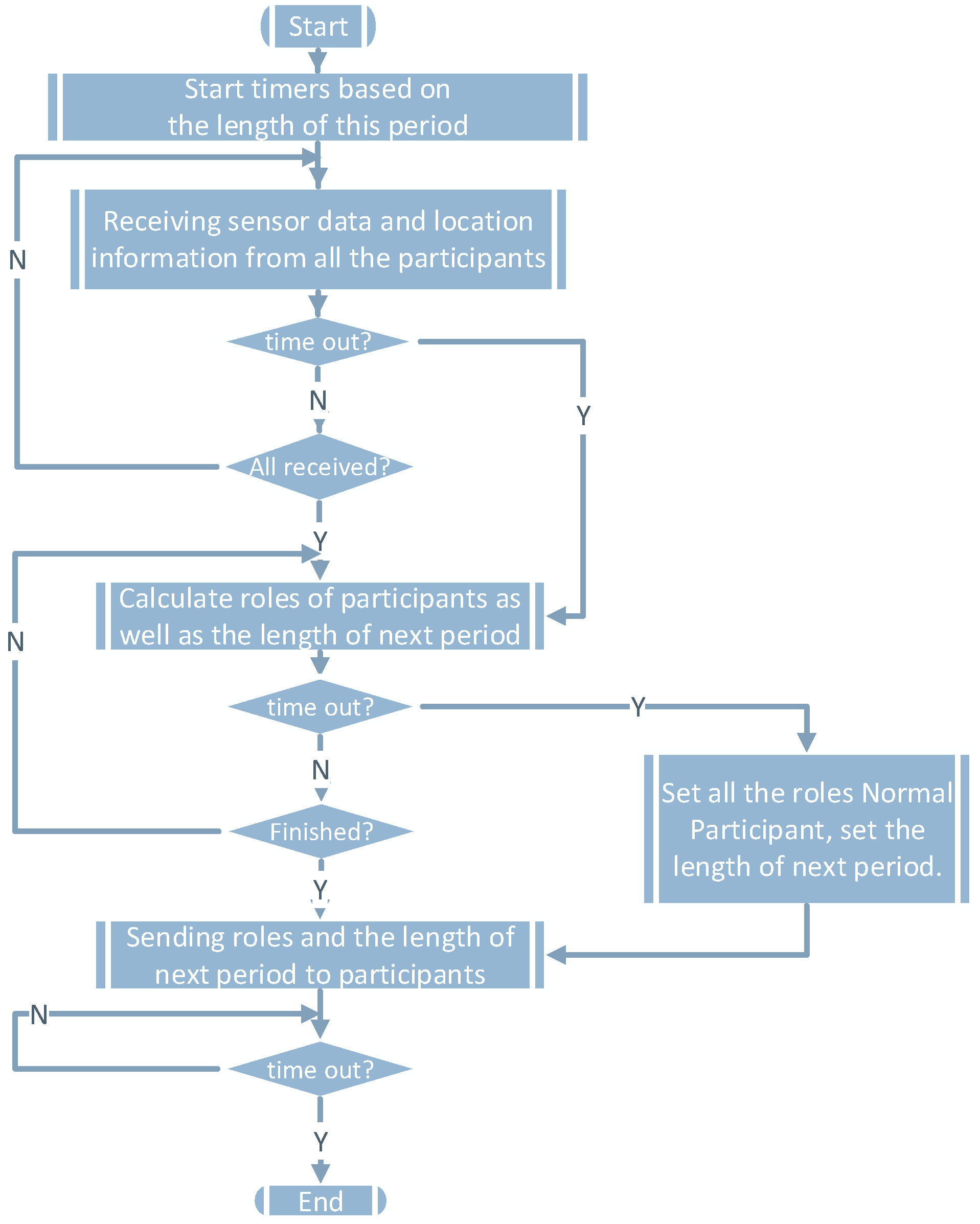
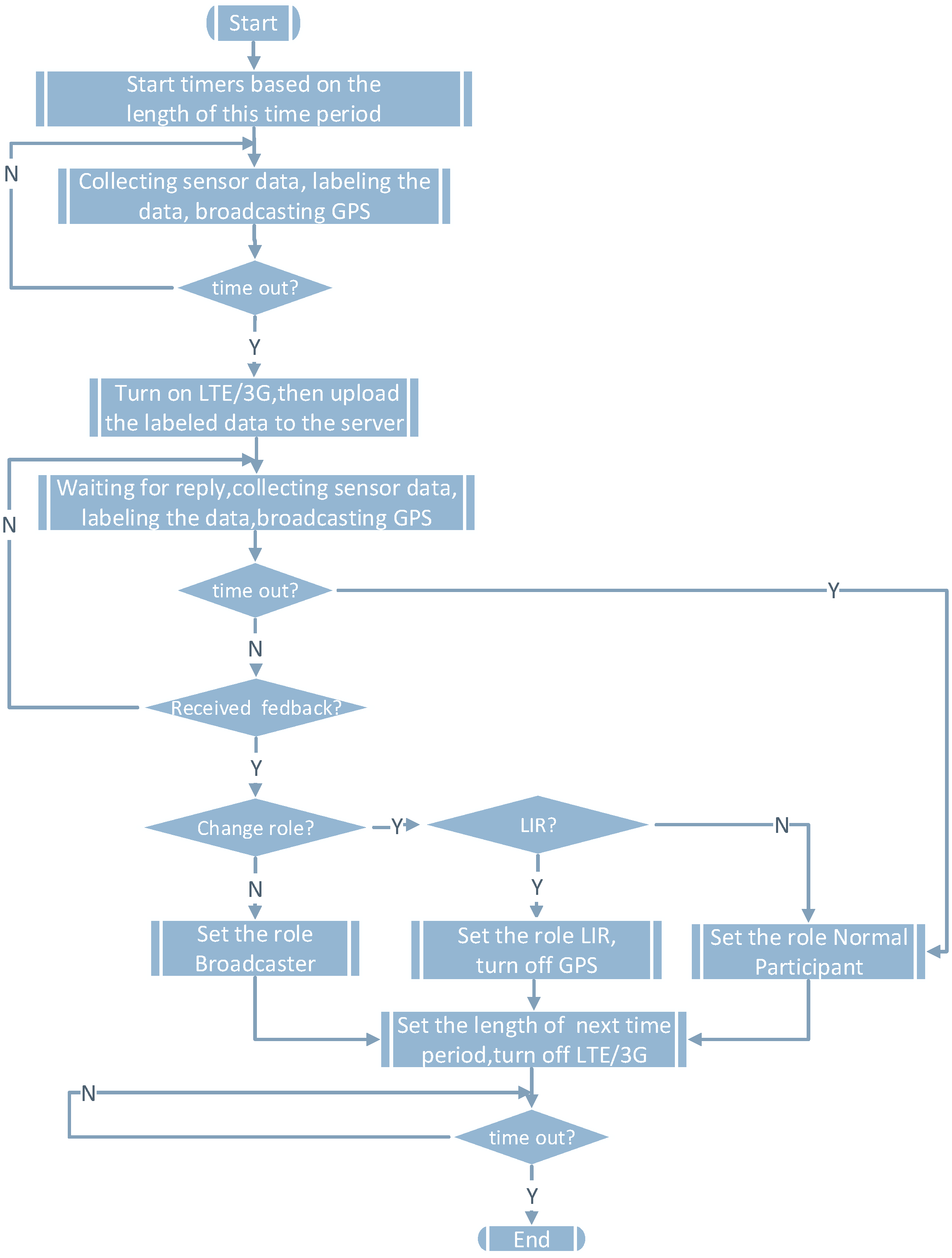
Figure 3 shows the corresponding function flow of the server. During [
], the server will decide on the roles of all participants in the next collaborative localization period and the length of the period. The goal is to minimize the power of all participants. Finally, the server will send the roles and the length of the next period to all participants. If the server does not receive sensor data from certain participants before timing out, the server will set the role of those participants as normal participants.
4. Modeling and Problem Formulation
In this section, we will present device to device localization. Then, we will model the energy consumption of different roles in our system. Finally, we will formulate the BSSP.
4.1. Device to Device Localization
This subsection shows how an LIR
j can calculate its location through the WiFi broadcast of a broadcaster
i, where
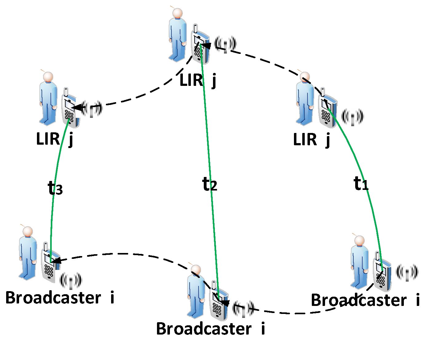
. Locations in the real world are measured in three dimensions, namely latitude, altitude and longitude. Without loss of generality and for simplicity, a two-dimensional scenario without the altitude dimensional is considered in this paper. As shown in
Figure 4, the scenario comprises two mobile devices held by the mobile users,
i and
j. The arrows indicate the trajectories of broadcaster
i and LIR
j.
The basic procedure of device to device localization can be divided into three phases, time stamped by , , , where ∈ and .
As mentioned before, broadcaster i broadcasts its location periodically. is the time when LIR j first receives i’s broadcast. Then, LIR j receives i’s broadcast the second and third times at and . The RSSI between i to j at time tis denoted by . The movement of participant i from to , in terms of the walking distance and heading angle, is denoted by a vector .
The relative movement between i and j from to is denoted by . The relative location of the LIR j towards the broadcaster i can be calculated as follows.
The movement measurement is based on the step detection method, which is commonly used in pedestrian localization [
20]. The pedestrian’s walking steps are detected by the acceleration signal, and the step length is estimated based on the statistical model. In each step, the walking direction is measured by the digital compass on the mobile devices. The nonlinear model [
21] is selected to estimate the step length. The step length
of pedestrians during [
,
] is determined by his accelerator readings:
where
represents the maximum acceleration during [
,
],
represents the minimum acceleration during [
,
] and
K is the coefficient.
Based on the counted number of steps, the estimated step length, the direction of each step and the movement vector of LIR
j can be calculated separately by:
where
is the angle between the
x-axis and the pedestrian’s heading direction measured by the geomagnetic sensor equipped by mobile devices and
is the number of measured steps during [
,
].
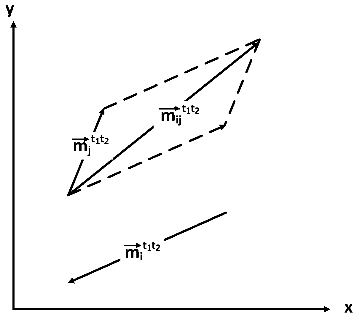
As shown by
Figure 5, the relative movement of LIR
j towards broadcaster
i from
to
,
, can be calculated by:
Let
be the distance between participants
i and
j at time
t and
=
be the distance matrix at time
t, such that:
According to the free space radio propagation model [
22], the relationship between
and
is denoted as:
where
n is a measure of the influence of obstacles, like partitions, walls and doors.
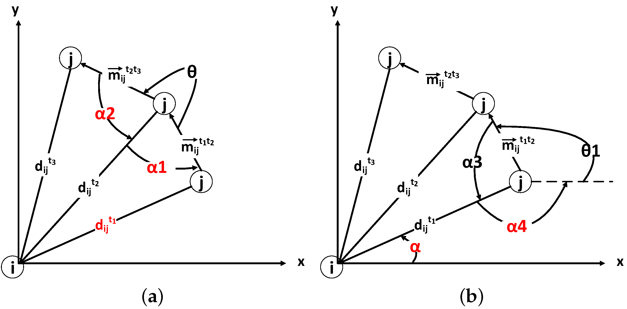
The problem is transformed as shown in
Figure 6. Broadcaster
i’s location at time
is set to be the origin of the coordinates. The
y-axis is pointing to the north, and the
x-axis is pointing to the east. The direction of
j towards
i at
is denoted by the angle
α (see
Figure 6b).
Let
and
denote the angle between
and
and the angle between
and
respectively, as shown in
Figure 6a. According to the cosine theorem,
and
can be expressed by:
The angle
θ between
and
can be calculated from
and
. Besides,
add up to
.
By differentiation, the derivative of Equation (10) is always positive. Thus, the sufficient conditions for the monotonicity of Equation (10) are fulfilled. The transcendental Equation (10) can be solved by the binary search method.
From
Figure 6b, we can easily see that
. The angle between
and
, denoted by
, can be calculated by:
Besides,
add up to
.
From the above, LIR
j can calculate its relative location to broadcaster
i at
. Given the location broadcast from
i, LIR
j can calculate its location at
. From Equation (
2), LIR
j knows
and
; thus, its location at
and
can be calculated.
Table 2, which is our preliminary results in [
19], shows the localization accuracy considering different distances between the broadcasters and the LIRs. When the localization accuracy requirement
r is higher, it requires a shorter distance
between the broadcasters and the LIRs. Note that the communication range of WiFi is denoted by
λ. When
r is greater than 25 m,
is equal to
λ meters.
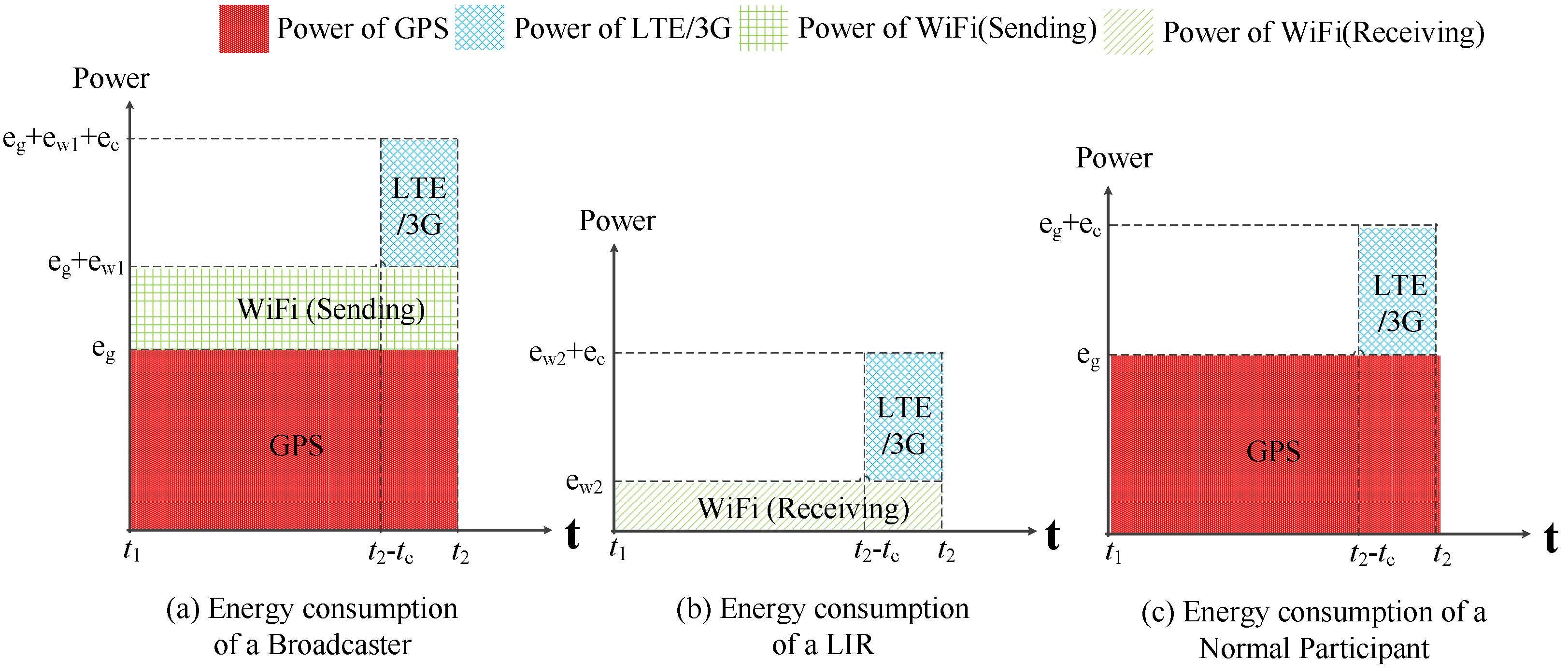
4.2. Energy Consumption Model
Let and be the power of GPS and the cellular network for localization, respectively. Let and be the power of WiFi communication for sending and receiving data, where . Then, we will study the power of mobile participants with different roles in collaborative localization.
Figure 7 shows the function flow of the broadcaster. During [
], the broadcaster uses GPS to obtain its location and uses WiFi to broadcast its location to the surrounding LIRs. During [
,
], the broadcaster uses the cellular network to report sensor data. We can easily model the energy consumption of the broadcaster during [
] in
Figure 8a. Similarly, we can illustrate the energy consumption of an LIR and a normal participant in
Figure 8b,c.
Let
be the power of a broadcaster for collaboration localization in [
], where ∀
,
∈
.
Let
be the power of an LIR during [
].
Let
be the power of a normal participant during [
].
We use Boolean to indicate whether a mobile participant m is a broadcaster during []. Similarly, we use Boolean to indicate whether a mobile participant m is a normal participant during .
Let
be the physical connectivity between participant
i and
j during
. Let
=
be the physical connectivity matrix during
, where:
The power of all of the participants during , , consists of three parts: the power of all of the broadcasters during this period (), the power of the LIRs () and the power of the normal participants (). We calculate these three parts in the following.
Given
and
, the power of all of the data broadcasters during this period can be calculated by:
According to
and
, we can get
. Thus, the power of all of the normal participants during this period can be calculated by:
For the remaining LIRs, their power during this period can be calculated by:
Finally, the power of all of the participants during this collaborative localization time period,
, can be calculated by:
4.3. Problem Formulation
The main goal of this work is to find an optimal broadcaster set and the length of each collaborative localization period, so that the power of all of the participants is minimized. To prevent some broadcasters from possibly consuming too much energy, our model considers the current remaining battery of participants, which is denoted by , . We formulate the BSSP in the following:
Minimize:
Equation (
21) is the integer constraint. Equations (
22)–(
24) calculate the power of the participants in the three different roles during
. Equation (
25) enforces that the remaining battery of each broadcaster must be above
μ. Equation (
26) enforces that the physical connectivity matrix of this period is determined by the current distance matrix, the length of this period, the location accuracy requirement of the task and the moving speed of pedestrian
v. Equation (
27) enforces that each LIR has to receive broadcasts from at least
h broadcasters so that it can calculate its location. In our proposed device to device localization method,
. It is worth noting that, simply by changing
and
h, other collaborative localization methods can also be represented by our proposed model.
5. Our Proposed Solutions
We propose two heuristic algorithms to solve the BSSP. The first one is a greedy-based broadcaster selection (GBS) algorithm. Algorithm 1 shows the pseudocode of the GBS algorithm. Based on the current distance matrix of all of the participants, the localization accuracy of the task and the moving speed of the pedestrian, GBS is able to get the approximate optimal set of broadcasters of the following collaborative localization period and the length of the following period.
Lines 9–29 show the inner while loop where the length of the period is fixed; thus, the solution is a local solution. We denote the power of participants in the local solution by . In the beginning, is empty, and equals . In each round of the while loop, the participant that saves the most energy will be selected as a new broadcaster during this fixed time period. The selection of broadcasters will continue until the power of all participants during this period, , cannot be further improved. After the while loop, we can get a local optimal broadcasters’ set under a given time . After the outer for loop (Lines 3–34) we can get the global optimal broadcasters’ set and its corresponding length of the period. By using , we can easily get the set of normal participants . The remaining participants, , are LIRs. All of the roles of the participants of the next period and the length of the next period are then calculated.
We also propose a simulated annealing (SA)-based [
23] broadcaster selection (SABS) algorithm. SA is a probabilistic algorithm that makes a good approximation to the global optimal solution of the optimization problem in a large search space.
The aim of the SABS is to get an approximate optimal set of broadcasters for the following collaborative localization period and the length of that period. The SABS algorithm includes a sub-algorithm called SubSABS.
Algorithm 2 shows the pseudocode of the SubSABS algorithm. SubSABS can find an approximate optimal only when the length of this period and the number of the broadcasters are given. Since the length of the period and the number of broadcasters during this period are fixed, the solution is a local solution. We denote the power of participants and the set of broadcasters in the local solution by and . Lines 1–7 are the initialization phase. Initially, it generates a feasible as the starting point. In each iteration of the outer while loop (Lines 8–30), a neighbor set of is generated, which is denoted by . If can save more energy than , then we accept as a new set of broadcasters. Otherwise, we accept based on the probability of avoiding falling into a local minimum. The probability of acceptance is an exponentially decreasing function with parameter , where is the current temperature. After each iteration, the probability of acceptance decreases. It can compute the suboptimal given specific and . This result will be used in the SABS algorithm.
![Sensors 16 00762 i001]() |
![Sensors 16 00762 i002]() |
Based on SubSABS, SABS can easily find the approximate optimal set of broadcasters for the following collaborative localization period and the length of that period. Algorithm 3 shows the pseudocode of the SABS algorithm. It can find an approximate solution by varying the number of broadcasters and calling the SubSABS algorithm. Even though the optimal is not known in advance, the SABS algorithm can find the approximate solution by calling the SubSABS algorithm times. After the outer for loop, SABS algorithm can find the approximate length of the next period and the set of broadcasters during this period . Similar to the GBS algorithm, based on , the roles of all participants in the next period can be calculated.
6. Performance Evaluation
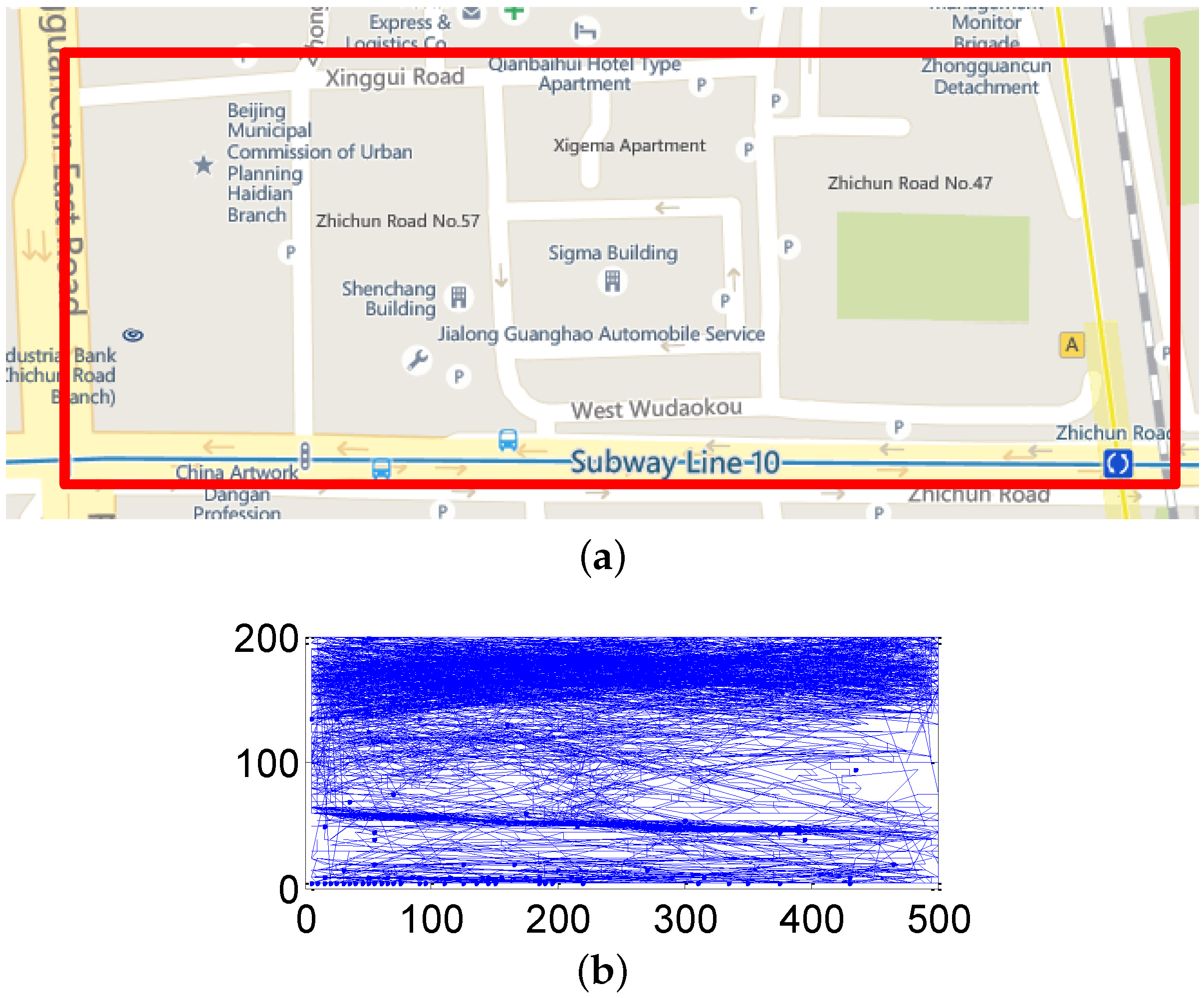
We evaluate the performance of the proposed collaborative strategy using the GeoLife (Microsoft Research Asia) dataset [
24], where real movement traces of ordinary citizens are used to represent mobile users in the considered scenario. The GeoLife project of Microsoft Research Asia has collected 182 volunteers’ (ordinary citizens) trajectories in Beijing from April 2007–August 2012. A GPS trajectory of this dataset is represented by a sequence of time-stamped points, each of which contains the information of latitude, longitude and altitude.
We store all of the trajectories in a geographical MySQL database and find a 200 × 500 m
region that is of high movement density, as shown in
Figure 9a.
There are 612 trajectories in this region, as shown in
Figure 9b. All 612 trajectories in the region are taken as mobile participants,
i.e., |
| = 612. Since a sensing task usually lasts for some time, some trajectories are too short to experiment. Thus, we choose the trajectories with a length longer than 20. After screening, there are 178 trajectories in total,
i.e., |
| = 178. We set the parameters in our energy model according to [
25,
26,
27], where
= 355 mW,
= 268 mW,
= 240 mW and
= 50 mW. As the GeoLife dataset does not provide battery information, we set
μ = 0%, which means that every participant has the possibility to be a broadcaster.
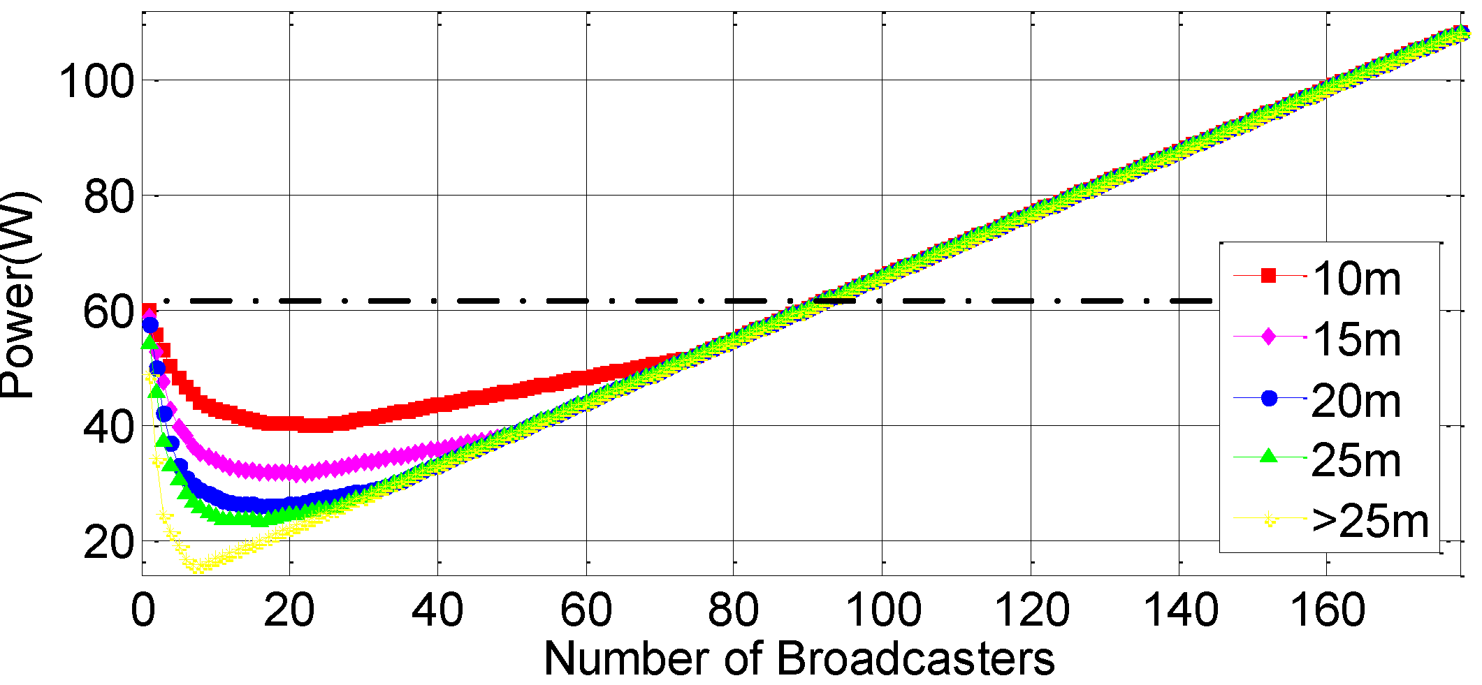
First, we evaluate how the number of broadcasters will influence the total power under different localization accuracy requirements. In this experiment,
is set to 20.
Figure 10 shows the power of all participants varying the number of broadcasters. Initially, the power decreases with the number of broadcasters. However, after reaching the optimal points, the power increases with the number of broadcasters. This is because excessive broadcasters consume energy for GPS localization and broadcasting their locations. The black dotted line in this figure shows the power of all participants without collaborative localization. We can see that if the broadcasters reach a certain number, collaborative localization does not save more energy than GPS localization.
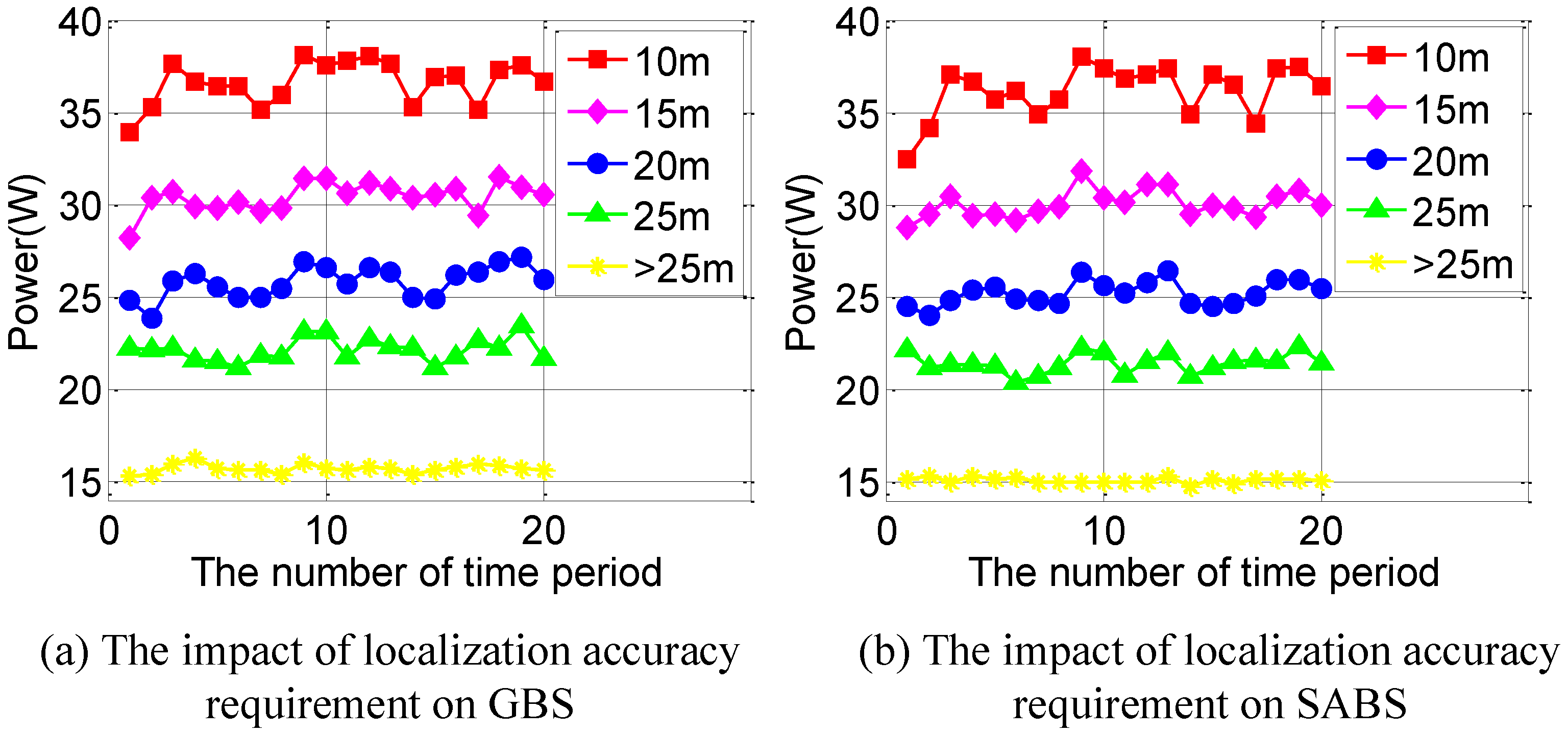
Next, we evaluate our proposed solution under different localization accuracy requirements.
Figure 11a,b shows the impact of localization accuracy on GBS and SABS. As the localization accuracy requirement increases, both the GBS and the SABS consume more energy. This is because more broadcasters are needed to satisfy the accuracy requirement. It is worth noting that GBS performs better than SABS in some cases. This is because the number of iterations of SubSABS is set to 5000. If we increase the number of iterations, SABS performs better than GBS in all cases.
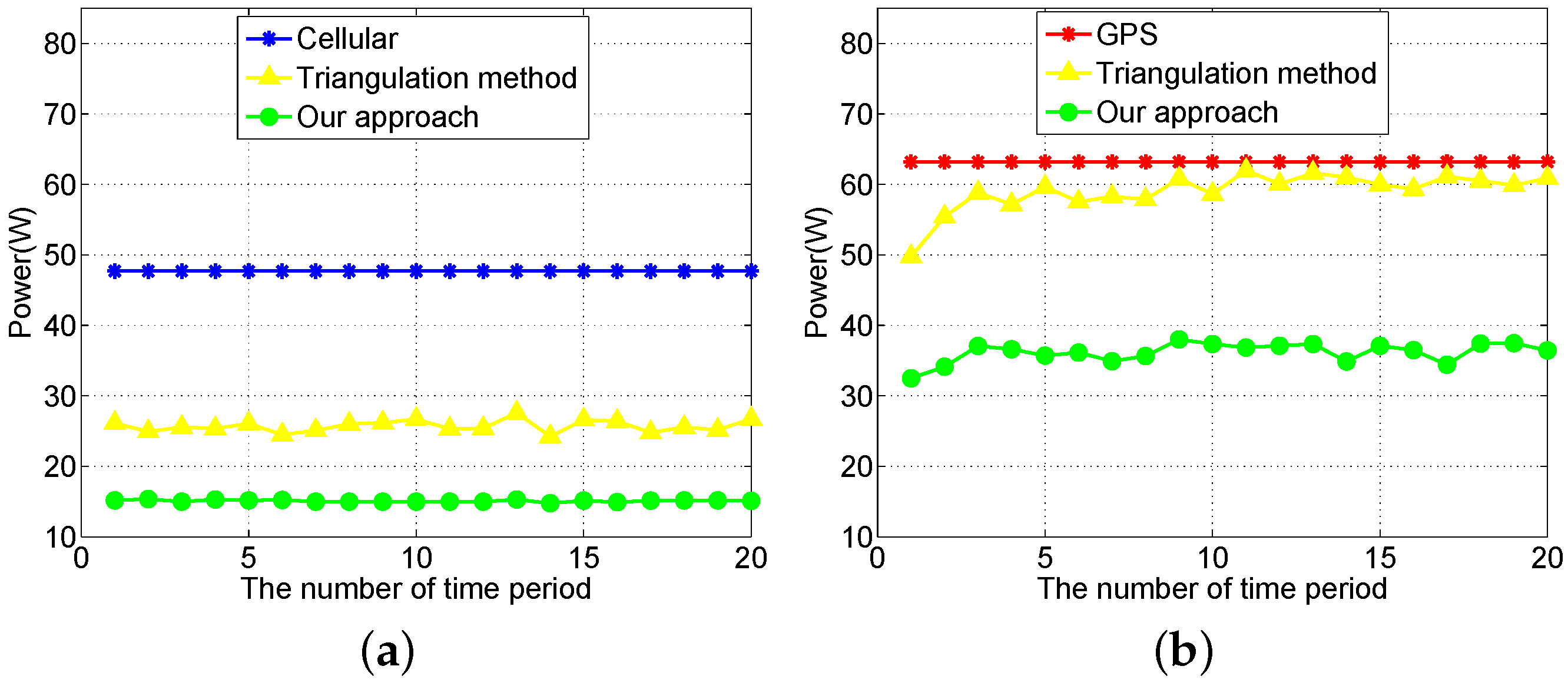
Then, we compare the power consumption of our approach to the existing solutions. We compare the standard triangulation method for collaborative localization with our proposed device to device localization method. When we use the triangulation method for collaborative localization, each LIR relies on three broadcasters’ locations to calculate its own location.
Figure 12a compares our approach to the cellular and triangulation method when the localization accuracy requirement is greater than 25 m. Our approach can save 68% and 41% energy on average compared to the cellular and triangulation localization methods, respectively.
Figure 12b compares the power consumption of our approach to the GPS sampling and triangulation method when the localization accuracy requirement is 10 m. In the traditional approach, all mobile participants turn on their GPS to perform localization periodically [
11,
28]. Our approach can save 43% and 38% of the energy on average compared to GPS and triangulation localization, respectively. In the best case, our approach can save 48% of the energy compared to GPS localization. In the worst case, our approach can save 40% of the energy compared to GPS localization.
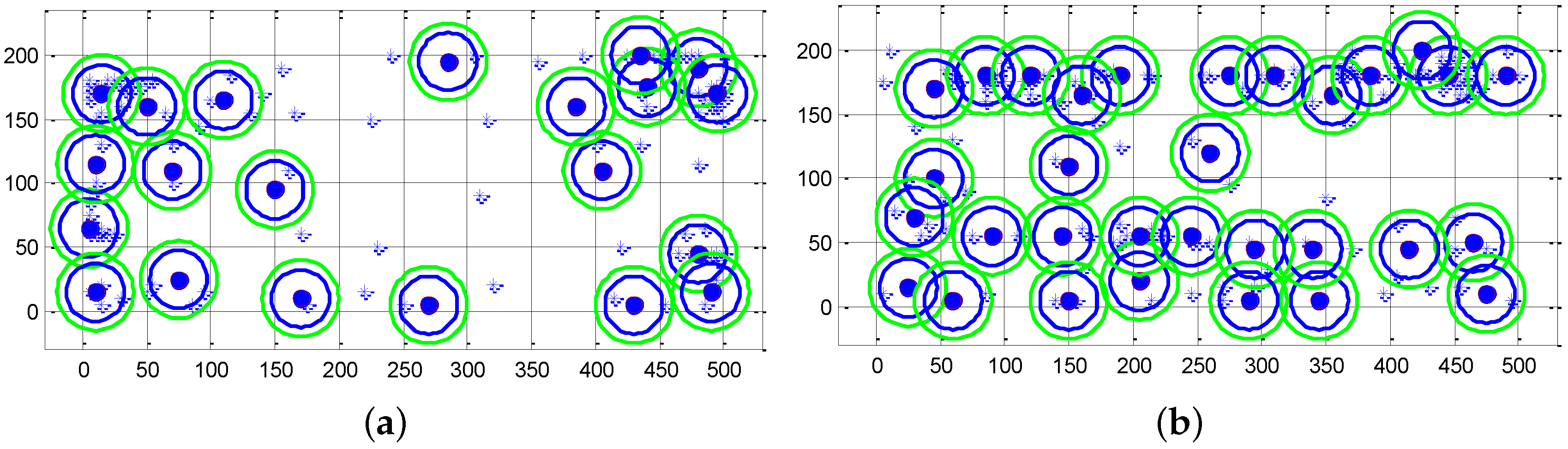
Figure 13a shows the time slice of user locations with maximum energy saving (the best case), while
Figure 13b shows the time slice with minimum energy saving (the worst case). The radius of the outer green circles in the figure is equal to
, which is the distance threshold corresponding to the localization accuracy requirement. The radius of the inner blue circles is equal to
, so that all of the LIRs within the blue circle will not move out of the green circle during a collaborative localization period, where
v is the moving speed of the pedestrian and
l is the length of the collaborative localization period.
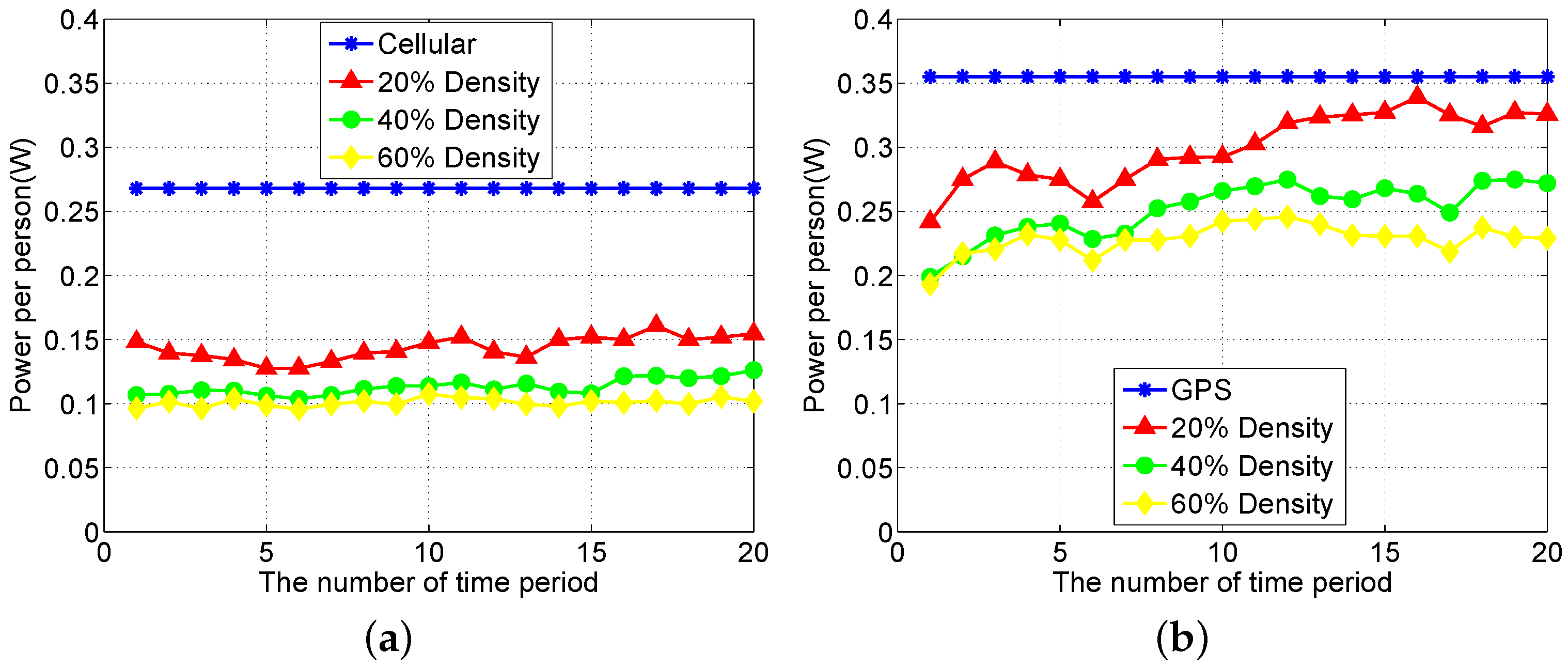
Furthermore, we study how the participant density will influence our proposed method. We choose 20%, 40% and 60% of the total participants to do the experiment, respectively. We choose the subsets of participants so that others can repeat this experiment. As the number of participants varies under different participant density, we evaluate the average power per participant during each time period.
Figure 14a shows the influence of participant density when the localization accuracy is greater than 25 m, while
Figure 14b shows the influence of participant density when the localization accuracy is 10 m. From
Figure 14, we can see that as the participant density increases, our method proposed performs better under both localization accuracy requirements.
Finally, we evaluate the performance of our proposed algorithm. In a specific case when
is set to
and the length of the time period is fixed, the BSSP can be converted to the well-known set cover problem (SCP), ∀
∈
. Then, we can get the optimal solution on the specific case using CPLEX 12.6 [
29]. In our experiment, the localization accuracy is set to 25 m, and
is set to 20. We choose the time slice with the most participants; then, we filter the participants who are at the same locations. Under this condition, there are 325 participants in total,
i.e., |
M| = 325.
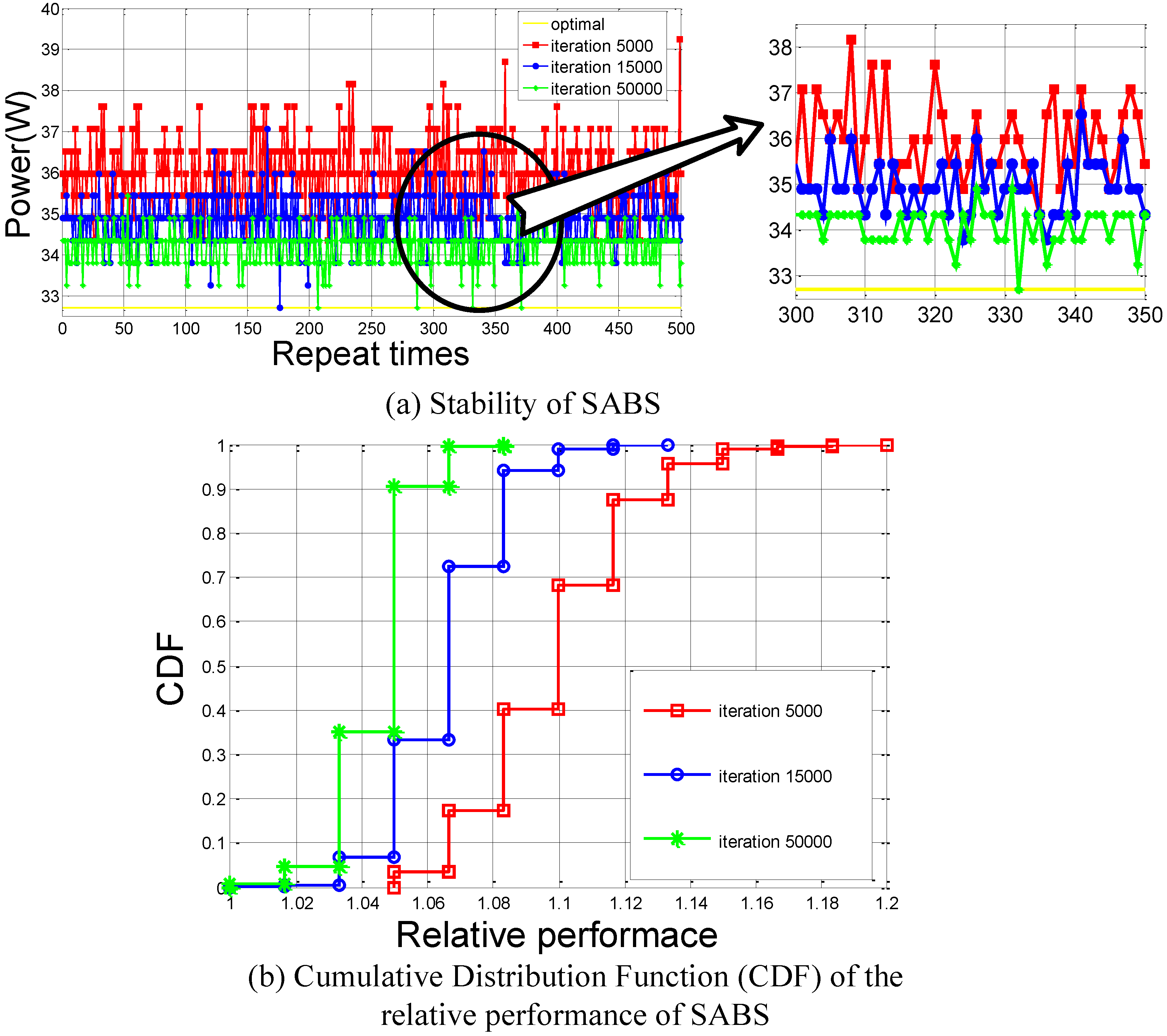
Figure 15a shows the stability of the SABS algorithm with different numbers of iterations. When the number of iterations is set to 5000, SABS is 90.2% to the optimal on average. When the number of iterations is set to 15,000, SABS is 93.4% to the optimal on average and has a probability of 0.2% to reach the optimal. When the number of iterations is set to 50,000, SABS is as close as 95.5% to the optimal on average. It has a probability of 0.8% to reach the optimal.
Figure 15b shows the cumulative distribution function (CDF) of the relative performance of the SABS algorithm with different numbers of iterations. As the number of iterations increases, SABS performs better. Even when the number of iterations is set to only 5000, our proposed solution is already much better than the existing solutions, as shown in
Figure 12.
In summary, our solution enables flexible adjustment on the localization accuracy according to the application requirement and minimizes the energy consumption for localization. Under all localization accuracy requirements, our approach performs better than the existing approaches.


