1. Introduction
Environment perception is a key research direction in the area of UGV development. The UGV is expected to navigate autonomously in semi-structured environments such as campus sites, parks, and the urban environment. It is important for an UGV to be able to detect obstacles around it correctly in order to avoid the risks of collision. The road curb is a special sub-category that can represent the boundary of the road so as to calculate the obstacle-free areas.
According to the different features of the curb detection, the existing algorithms are divided into two categories: the first is based on detection of the geometrical features of the curb; the second category is based on image context derived from the monocular vision field. The main merit of the second method is that it contains rich information, such as color, texture,
etc. Commercial lane departure warning systems based on monocular vision are available now [
1,
2]. However, the method belongs to the first category which has problems to cope with bad situations such as poor illumination, bad weather and insufficient road lanes. Compared with the second category, in general, the first category is not affected by the above factors, except stereo vision, and is adaptive and robust to the varied environment. Therefore, we will concentrate on the first category of algorithms in this research.
The geometrical features of a curb are not clear in a real structural environment, as curb height varies only from 5 cm to 25 cm in general. Therefore, curb detection is a challenging task, because the geometrical features of a curb might be contaminated by random noise and measurement errors. In recent years, researchers have presented some curb detection algorithms using geometrical features which are obtained by laser range finder [
3–
8], stereo vision [
9–
11], TOF Camera [
12,
13] and structure light [
14]. According to the idea of curb detection, such algorithms can be divided into two classes: one idea is that range data is processed individually per frame and the algorithm can obtain curb candidate points, then the curb points are tracked using the filter method, such as Kalman filter and Extend Kalman filter; the other idea is that the algorithm extracts ground surface or obstacle-free area in a local map to obtain local curb information.
In [
3,
4], Kodagoda
et al. used a tilted 2D laser range finder to detect road curbs. In this approach, the result of the measurement is predicted with the Kalman filter algorithm. If the measurement is far away from the prediction, it is considered as a curb candidate. Prior knowledge assumptions have to be made to find the right curbs. For example, the UGV needs to move in parallel to the curb, the street width is known, and the curbs are locally straight. Furthermore, Kodagoda
et al. proposed an effective curb tracking and estimation method with camera and laser range finder data in [
5]. Smadja
et al. [
6] also presented a curb detection approach using a 2D laser range finder. Firstly, the road surface points are extracted by the RANSAC algorithm and are projected onto a global map; secondly, the boundaries of the obstacle-free area are fitted by the RANSAC algorithm, and then the curb candidate points are picked out by a multi-frame accumulated map. In [
7], the author detected road curbs using HDL64-E LIDAR which contains 64 scan lines, but the algorithm deals with the data to be one line as a unit. Zhang proposed a road boundary method which are extracted using the elevation information based on the single data frame from the 2D laser range finder in [
8], and the method had been verified in the 2007 DARPA Urban Challenge. The ideas of the above curb algorithms belong to the first class algorithms based on geometrical features.
In [
9,
11], the stereo vision is used for detecting curbs. A straight curb is detected by the Hough transform, and a curved curb is extracted by chains of segments in [
9]. In [
11], the author changed the curbs model to cubic polynomial curves, and then used the RANSAC algorithm to compute the parameters of the model. The authors built a DEM to detect curbs by Conditional Random Field (CRF) in [
10]. The approach can detect and reconstruct different curvature and height curbs, but the algorithm assumes that the curb is visible in front of the vehicle. If the curb is occluded by another object on the road, the performance of the algorithm will be decrease. Gallo
et al. [
12,
13] proposed a modified RANSAC algorithm (dubbed CC-RANSAC) for detecting street surface and pavement surface using a Canesta TOF Camera. The algorithm can detect two nearby surfaces by the largest connected components of inliers. The above approaches [
9–
13] belong to the second class algorithms based on geometrical feature.
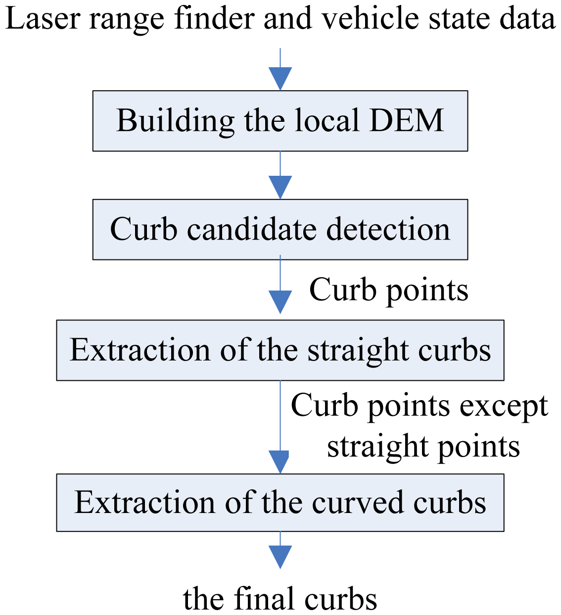
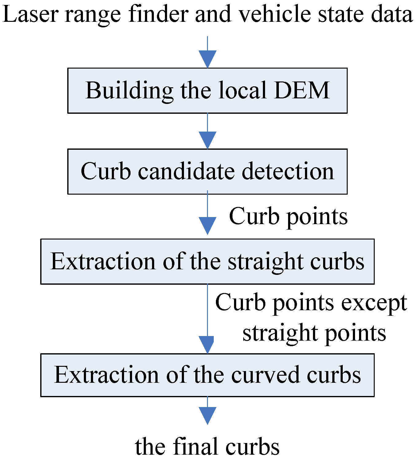
In this paper, we propose a new curb detection method based on a local DEM which is built from 2D sequential laser range finder data and vehicle state data. The algorithm can detect road curbs accurately and quickly in both static and typical dynamic environments where a few objects may move on the road or roadside, and it belongs to the second class based on geometrical feature algorithms. Compared with the first class algorithms, our method has three main merits. Firstly, our method can obtain robust curb detection results, because the historical and current sensor information is considered in the process of the curb detection. To be precise, our method uses the local DEM information which includes multiple laser data frames to detect the curb. The first class algorithms only use limited information, so these algorithms are sensitive to data noise. Secondly, we only select the suitable curb model in our method, and the curb tracking step is not available. The reason is that the curb model implies knowledge of the geometric information of the road. If we obtain the parameters of the curb model, we will not need to track the new curb. However, curb tracking is an important step after the curb detection in the first class algorithms, because it can check the validation of the new result based on the filter which includes the former curb information. In general, curb tracking is a difficult task using the traditional tracking methods such as the Kalman filter. The main reason is that the traditional tracking methods need to know the accurate process model and estimate the error model, which are hard to obtain in practice. Thirdly, our method can detect the curbs in a typical dynamic environment, which reduces the influence of moving objects in the process of the building the local DEM.
The paper is structured as follows: in Section 2, the proposed method is described, and the curb detection algorithm will be presented; the experimental results are shown in Section 3 and conclusions in Section 4.
3. Experiments
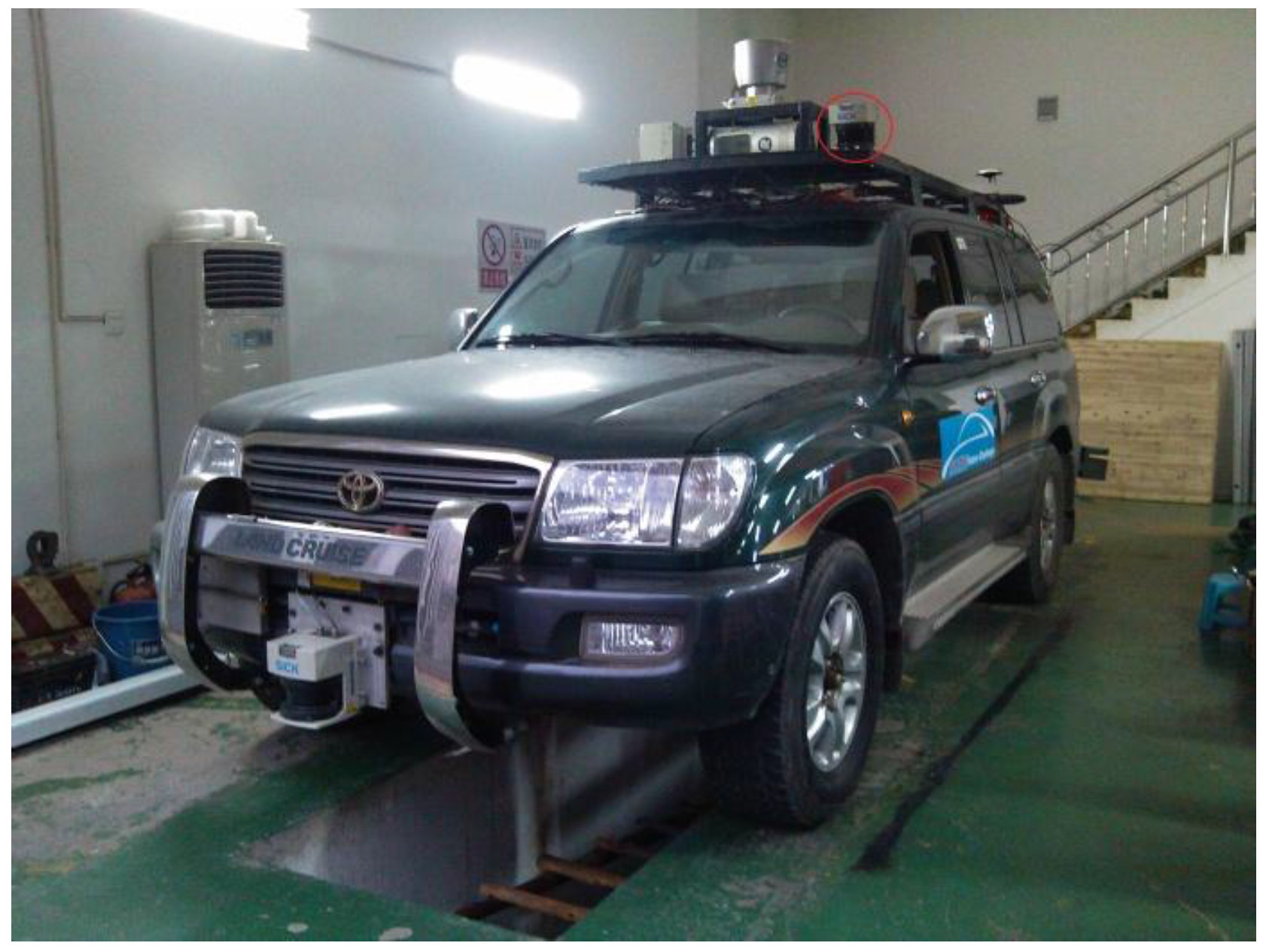
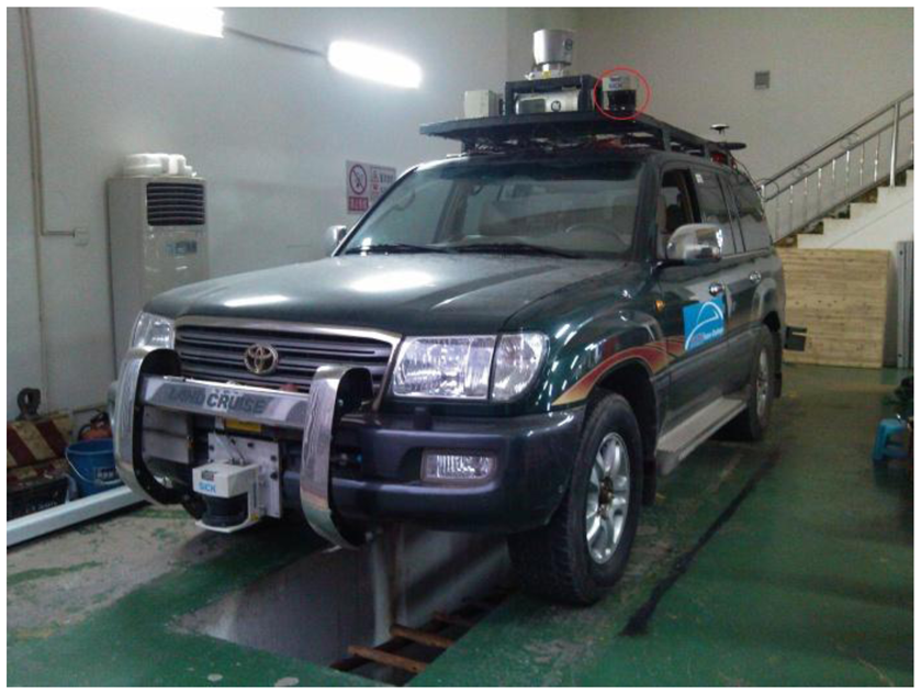
The experimental platform is a light off-road vehicle. A forward-looking laser range finder is mounted on the front top of the vehicle and tilts down a little, and it is shown in the red ellipse area in
Figure 9. The LMS-291 SICK sensor and SPAN-CPT integrated navigation system produced by the NovAtel Company were used in the experiment. The LMS-291 scans 180° field-of-view with 1° resolution at a 75 Hz scan rate, and the work mode is the interlace mode [
18]. It was installed at the height of 2 m to scan the road surface about 17 m ahead. The SPAN-CPT system used the DGPS mode in the experiment. The experiments were done on our campus. There are two experiments in this part. The first experiment is to verify the effectiveness of our algorithm. The second experiment is to analyze the results of our algorithm quantitatively.
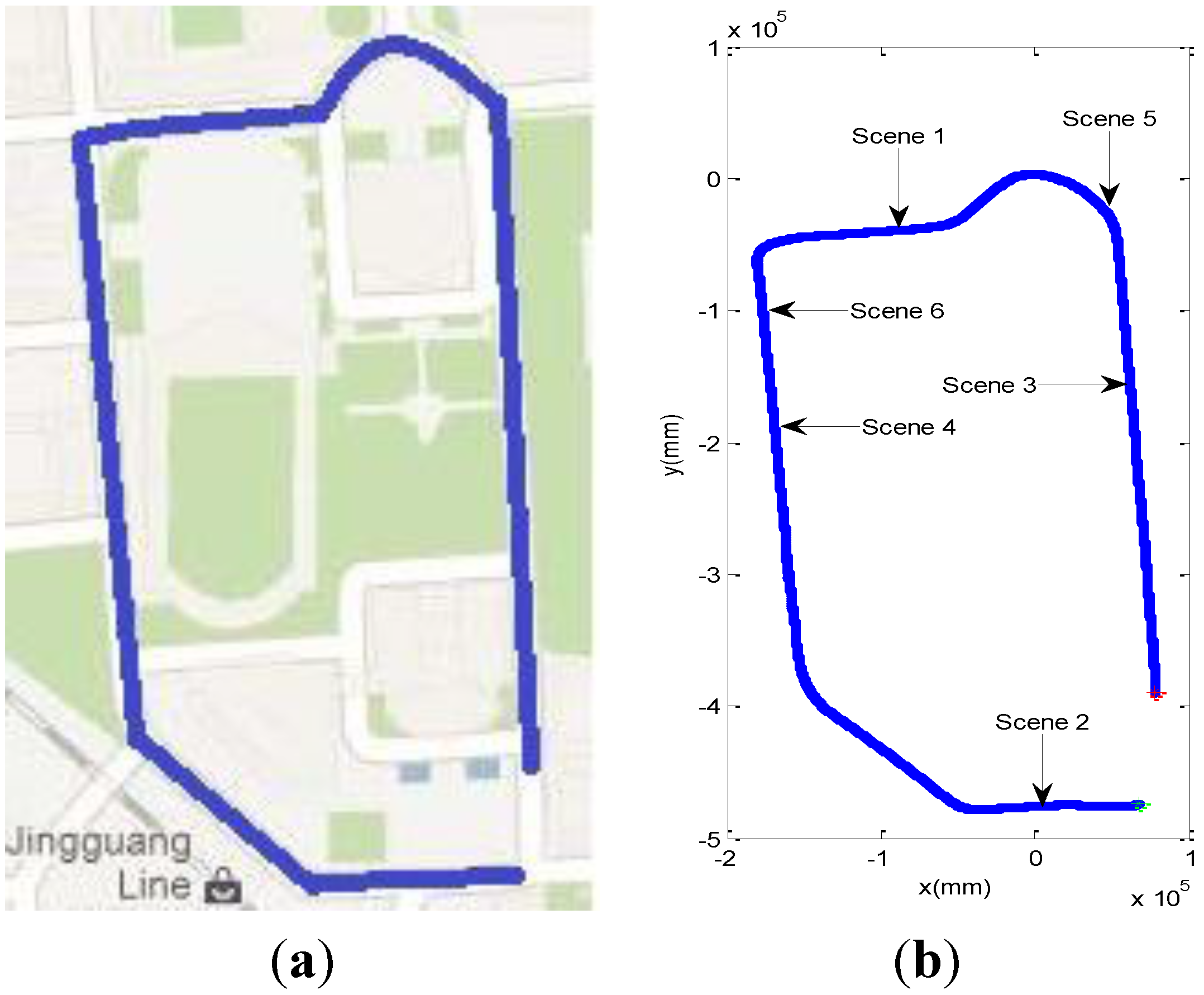
The first experimental site is shown in
Figure 10(a). The blue lines denote the route of the vehicle in
Figure 10, which are recorded from the navigation system of our vehicle. The travelled distance of the vehicle is 1.6 km. We select four typical scenes from the whole data set, and the positions of these four scenes are shown in
Figure 10(b). The red point denotes the start point of the vehicle, and the green point denotes the end point of the vehicle. The experimental results of six scenes will be introduced respectively in the following.
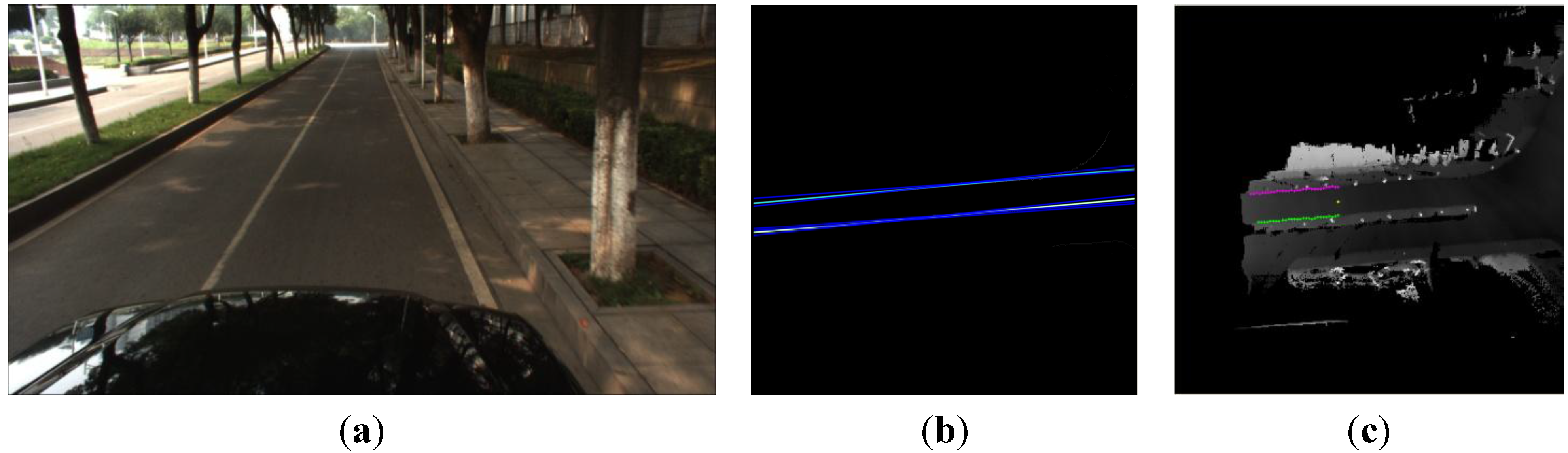
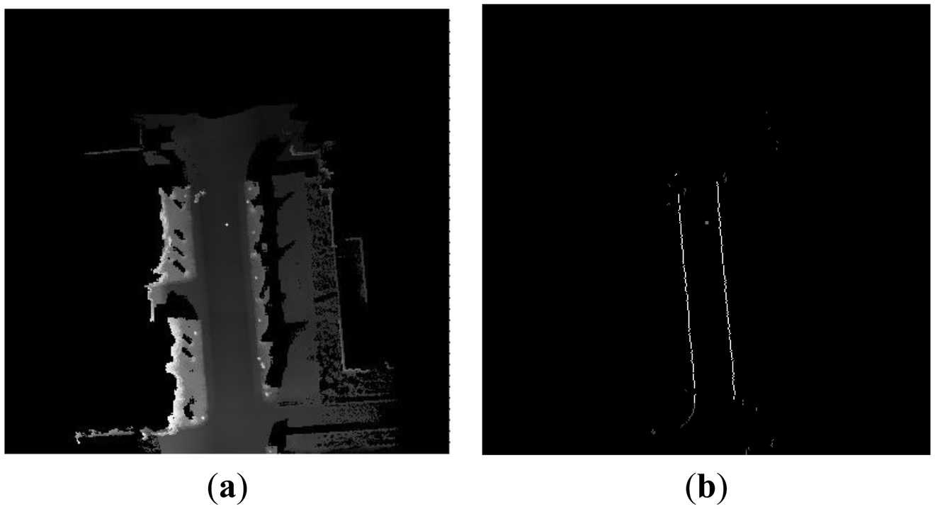
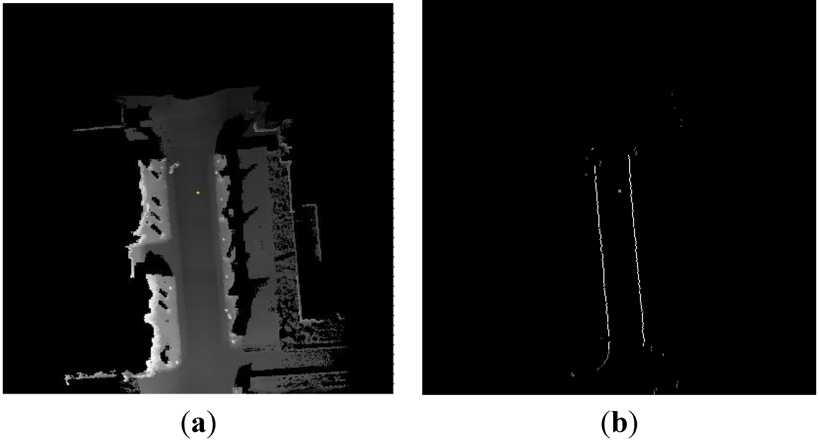
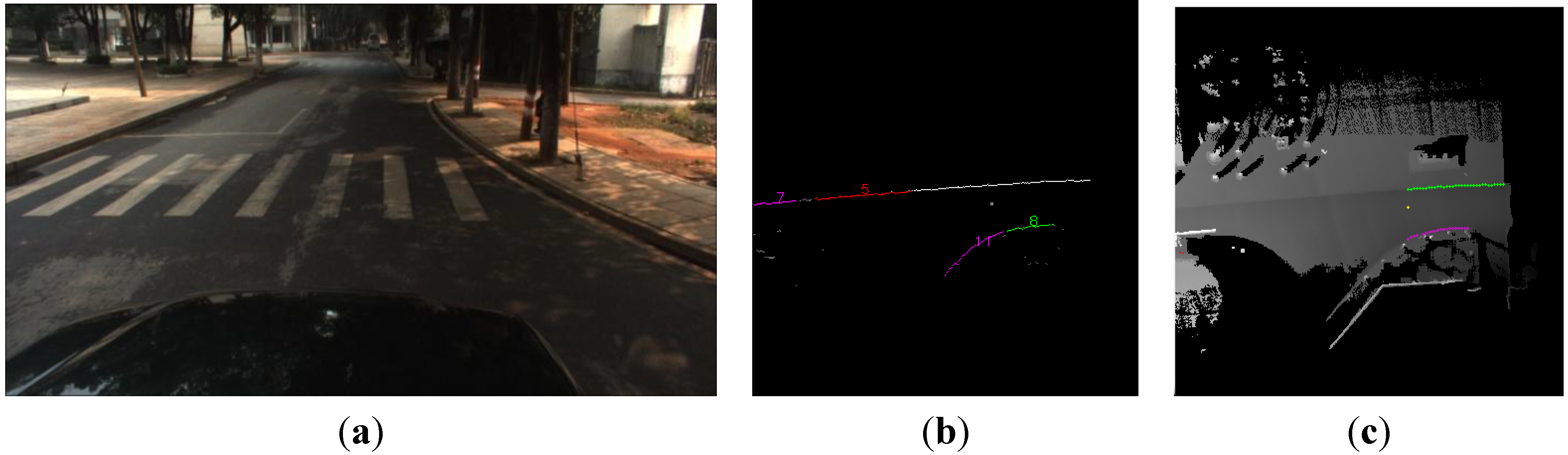
Typical straight curbs exist in Scene 1, and the vehicle drove from the East to the West.
Figure 11(a) presents the corresponding visual image in front of the vehicle and the two obvious straight curbs were seen in
Figure 11(a). The line detection result using the Hough transform is shown in
Figure 11(b). There are four lines in
Figure 11(b), the two white lines are selected as the results according to the constraint condition in Section 3.2.1.
Figure 11(c) shows the final straight curb result. The yellow points denote the position of the vehicle, the green points denote the detected left curb points and the pink points denote the detected right curb points. Our algorithm can detect the straight curb on the road accurately.
In Scene 2, the right curved curb and the left straight curb were seen in
Figure 12(a), and the vehicle drove from the West to the East. The data cluster result is shown in
Figure 12(b). The different colored points represent the different classes which not include the whole cluster result and only useful classes except the gray points which are unclassified.
Figure 12(c) shows the final curb detection result. The right curved curb is detected by our curved curb algorithm, and the left straight curb is detected by our straight curb algorithm. It has been verified that the proposed algorithm can detect curved curbs successfully.
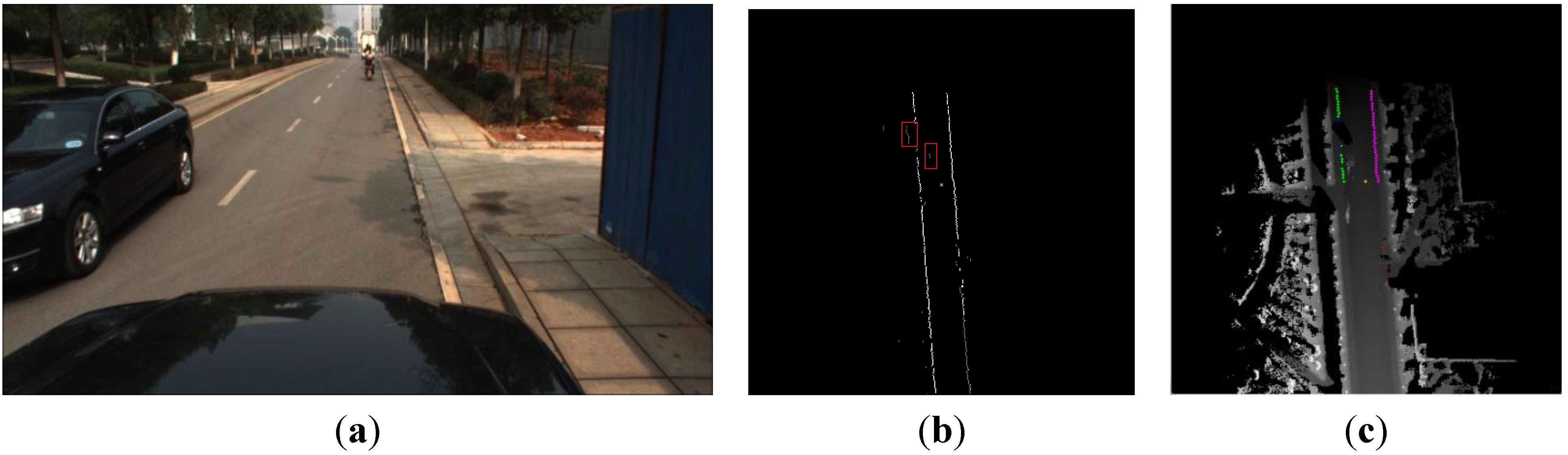
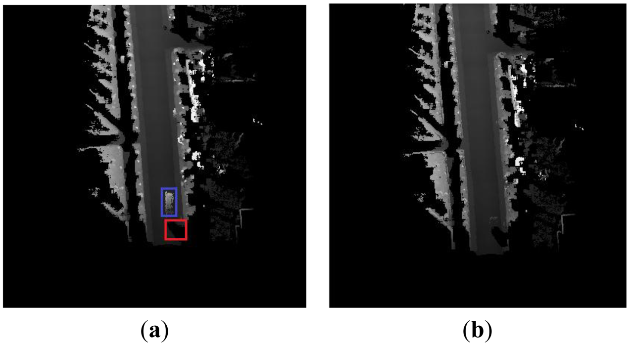
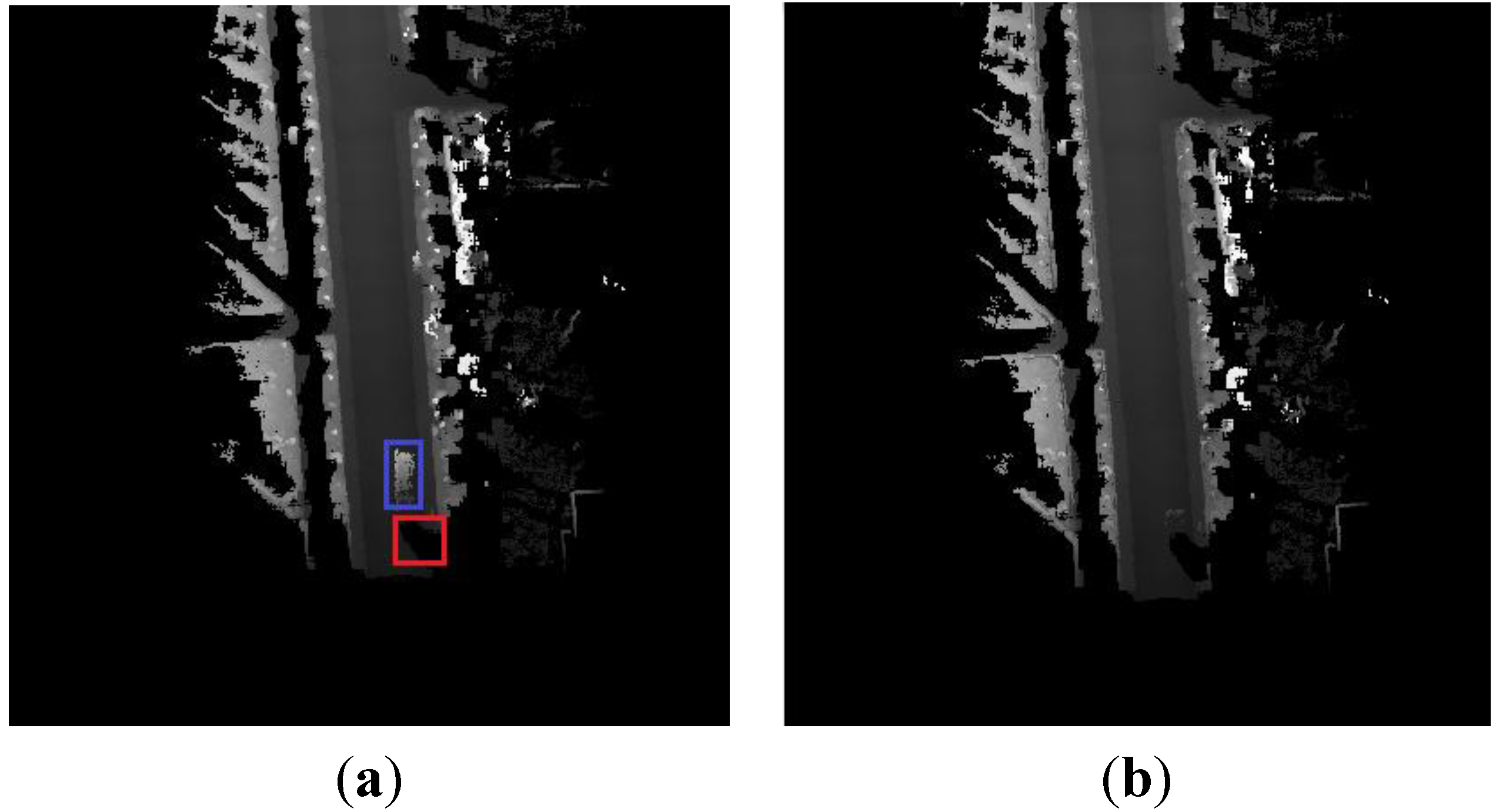
Scene 3 is a typical dynamic environment, and vehicle can be seen on the road in
Figure 13(a). Because the moving vehicle partly occluded the left road curb, missing data appeared in
Figure 13(c). In
Figure 13(b), the two red rectangles are some wrong results in the result of accumulated curb candidates. The left wrong result was caused by the missing data so the algorithm actually detected the roadside vegetation. The right wrong result was caused by the process of building the DEM due to the interference of the moving vehicle. In this situation, the difficulty of the curb detection increased, but the proposed algorithm can detect the left straight curb except for the region of the missing data.
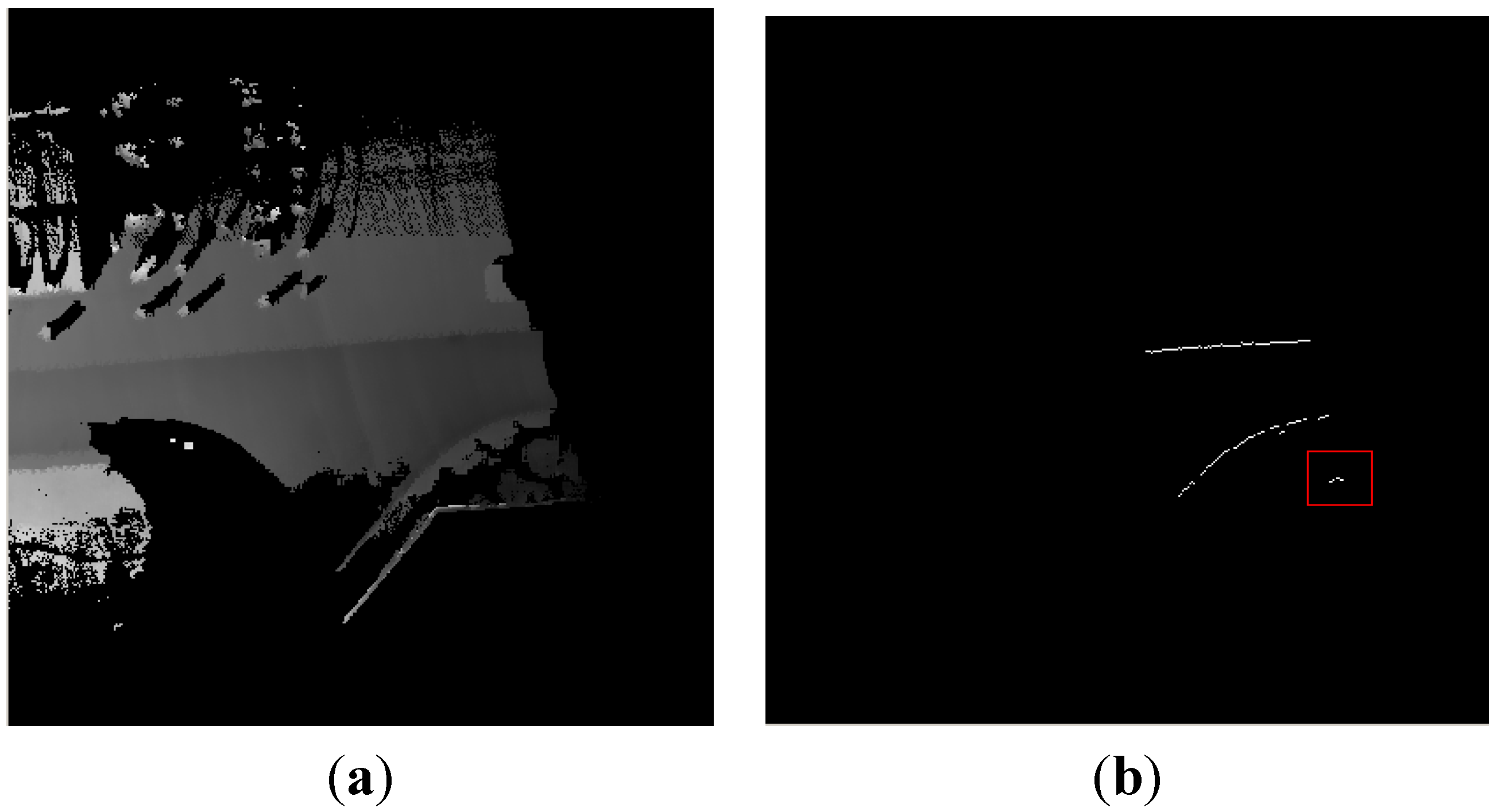
Scene 4 is a typical dynamic environment too, but it is more complex than Scene 3. Some dynamic objects which include the car and the bicycles appear in the local DEM in
Figure 14(a). Because of this, a lot of spurious objects appeared in the local DEM in
Figure 14(a), because the effect of the moving objects is not considered. We can find that the obvious error of curb detection appears in red rectangle area in
Figure 14(a). The above error arises from the spurious objects. The local DEM was built by our approach in
Figure 14(b), and the spurious objects are decreased, so we obtain a good curb detection result. All in all, our proposed algorithm can reduce the effect of moving objects and build a good quality DEM for use in detecting the curbs.
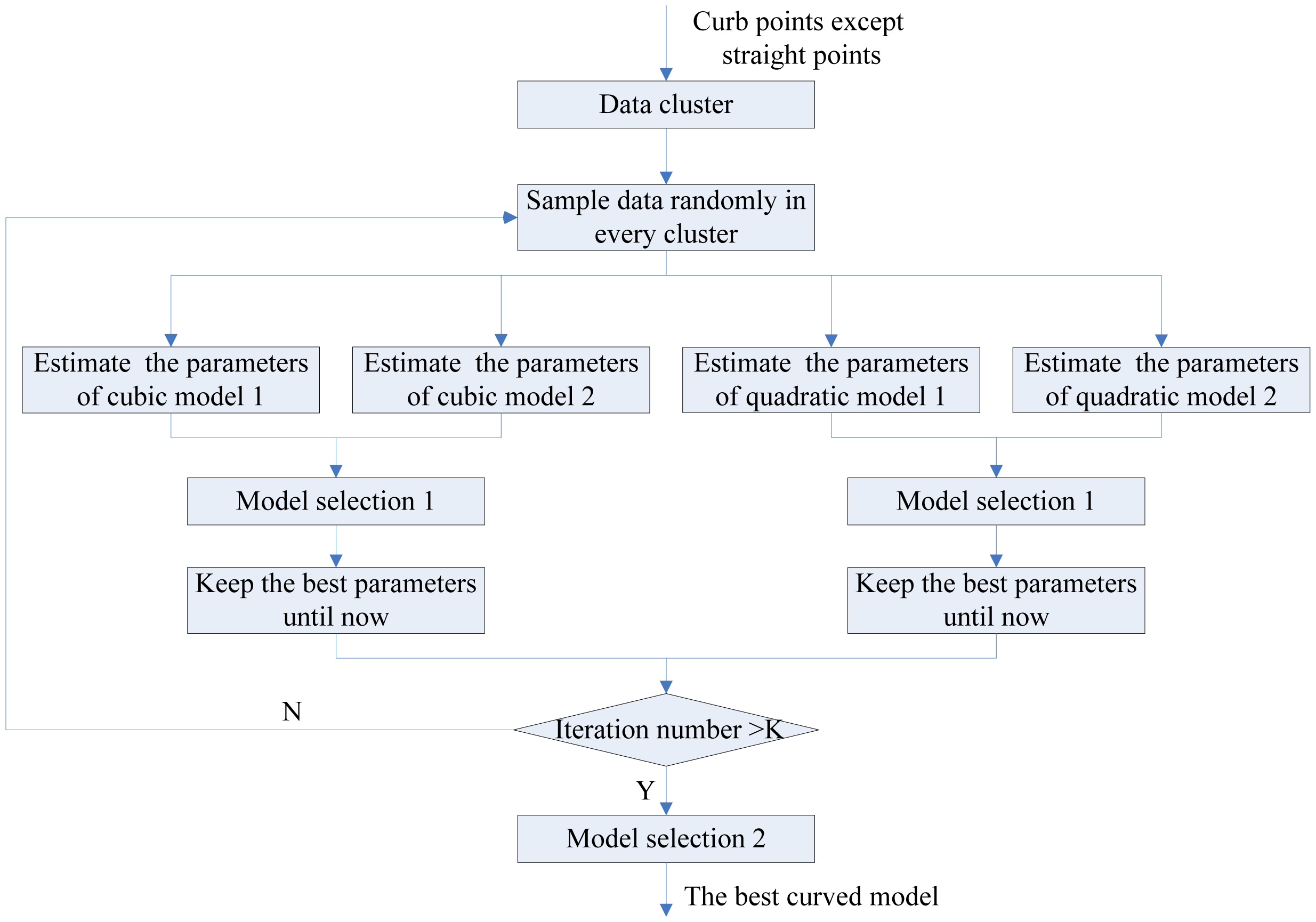
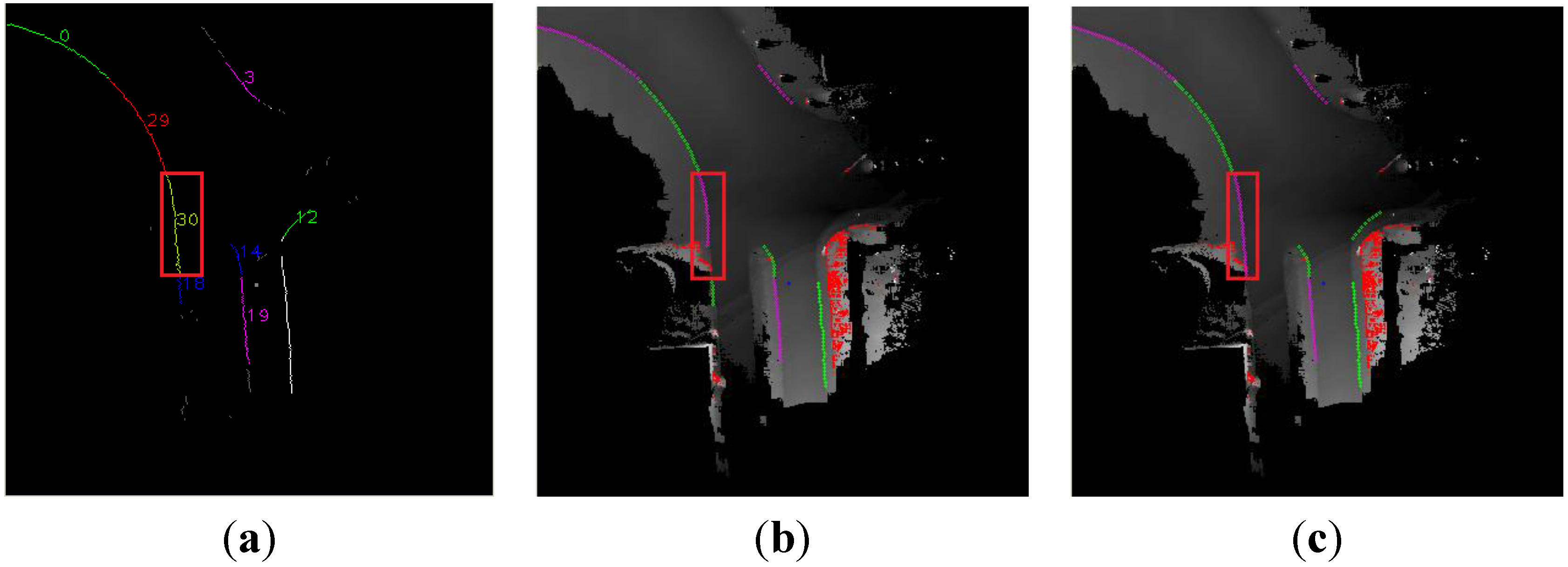
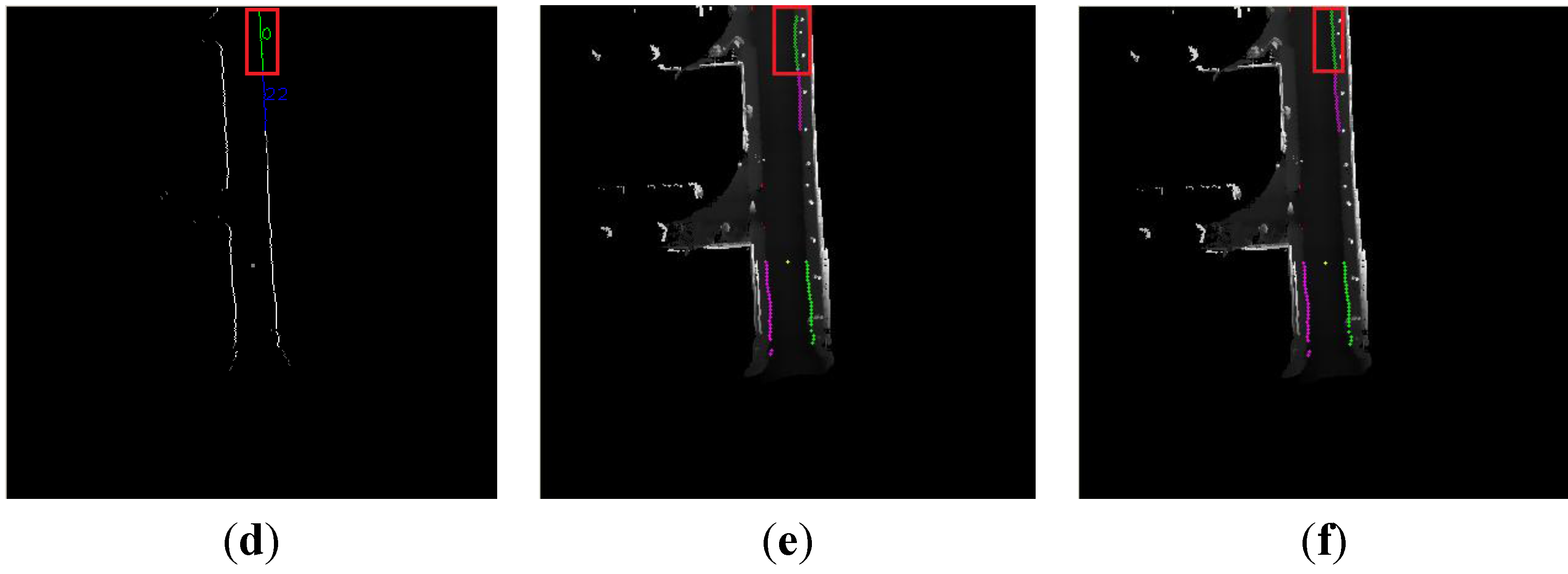
In [
10], the authors used a cubic polynomial model to represent the curved curb. In some cases, the cubic polynomial curve is unsuitable, that is to say the model cannot fit the curved curb well. Compared with the above methods, we select the quadratic polynomial model and cubic polynomial model to represent the curved curb in the multi-model RANSAC algorithm. The contrastive results of the curved curb detection are shown in
Figure 15, and results of the first row and the second row are detected in Scene 5 and Scene 6 respectively.
The results of the data cluster, bad detection and our algorithm are shown in the first, second and third column respectively. The red rectangle region denotes the same cluster in the same row. We use the quadratic polynomial model to obtain the result in
Figure 15(b). Compared with
Figure 15(a), the result lost the bottom data in red rectangle region in
Figure 15(b). In
Figure 15(e), the cubic polynomial model which is used in [
10] obtains a bad result which missed the upper data in red rectangle region, but our algorithm can obtain the best curved curb in
Figure 15(c,f). In short, our algorithm can select a better curved curb model than the algorithm in [
10], and obtain good results.
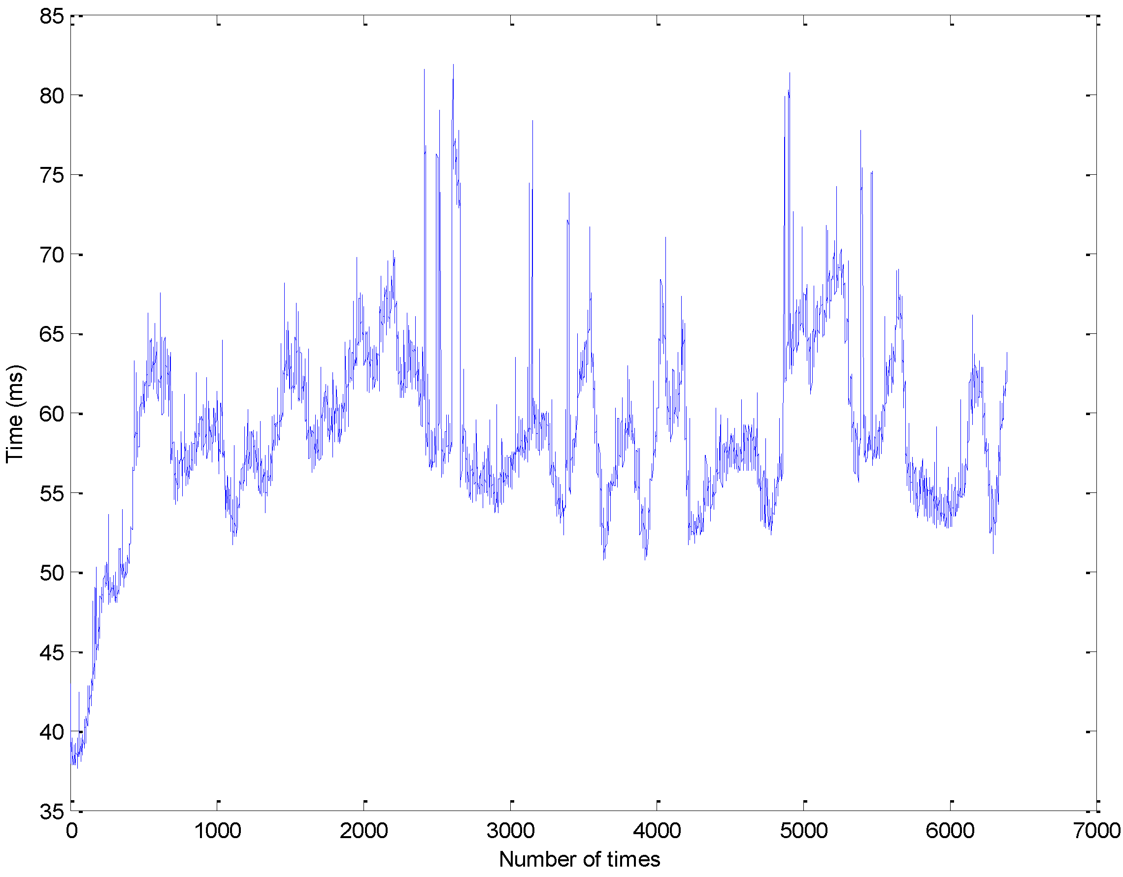
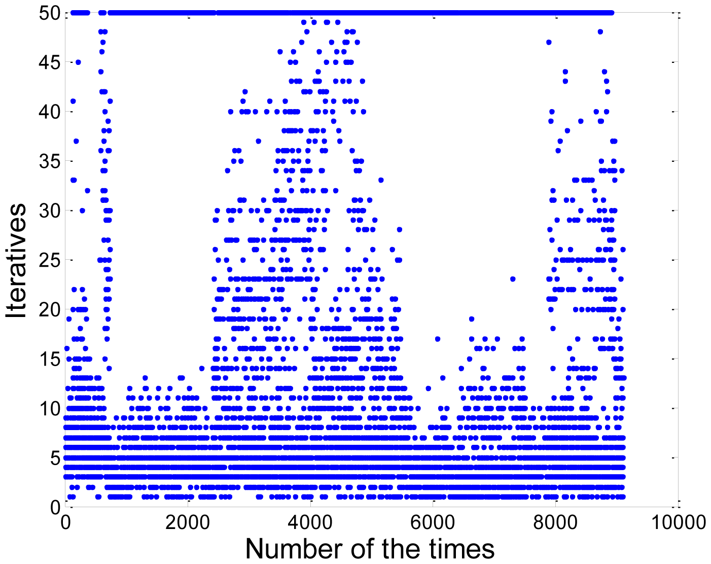
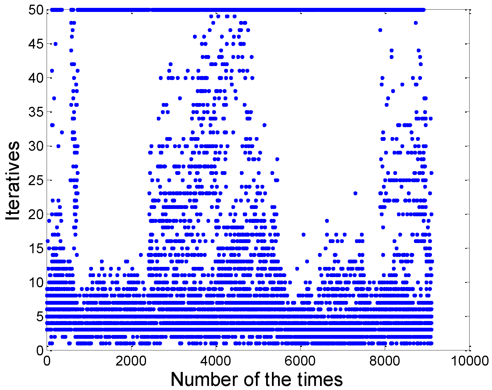
In the second experiment, the travelled distance of the vehicle is 3.2 km. The hardware and software specification in our system is shown in
Table 1. The execution time of our algorithm in the second experiment is shown in
Figure 16.
The average and the worst computational time of our algorithm are about 58.5 ms and 81.9 ms, respectively. In
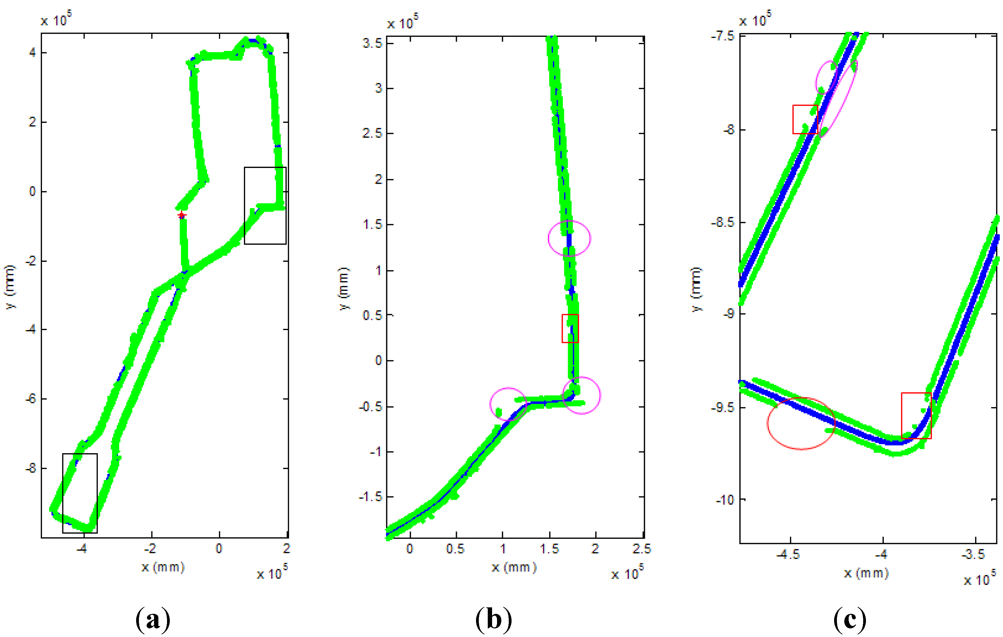
Figure 17, the curb detection results and the route of the vehicle is shown in the global coordinate system.
Figure 17(a) is the entire curb detection results in the second experiment. The top and bottom black rectangle areas are enlarged in
Figure 17(b,c), respectively. The blue lines denote the route of the vehicle, which are recorded from the navigation system of our vehicle, and the green points denote the detected curb points. The red rectangles and the purple ellipses denote the lost curb areas and the no curb areas which usually are the intersections on the road in
Figure 17(b,c). The confusion matrix of the second experiment is shown in
Table 2, and the data of the ground truth are labeled manually. Base on it, the true positive ratio and the true negative ratio are 86.8% and 93.4%. The accuracy of our algorithm is 87.8%. There are two reasons to the lost and wrong curb detection results. Firstly, the road structure is complex in our campus. There are many small intersections. Secondly, the curb candidate detection will lost some curb points, because the height of the curb changes a lot in different place. Thirdly, the laser data will miss in the water hole area on the road.


