

Research on the Prediction of Wax Deposition Thickness on Pipe Walls Based on the Optimal Weighted Combination Model
1
College of Petroleum Engineering, Xi’an Shiyou University, Xi’an 710065, China
2
Shaanxi Key Laboratory of Advanced Stimulation Technology for Oil & Gas Reservoirs, Xi’an 710065, China
3
China Petroleum Engineering & Construction Southwest Company, Chengdu 610041, China
4
SINO-Pipeline International, Beijing 102200, China
*
Author to whom correspondence should be addressed.
Processes 2023, 11(12), 3363; https://doi.org/10.3390/pr11123363
Submission received: 26 July 2023
/
Revised: 19 September 2023
/
Accepted: 19 October 2023
/
Published: 4 December 2023
(This article belongs to the Special Issue Risk Assessment and Reliability Engineering of Process Operations)
Abstract
:Wax deposition seriously affects the safe and economic operation of pipelines. Mastering the variation laws of wax deposition thickness is the premise of formulating reasonable pigging schemes. Although the GM (1,1) model (a kind of gray model) is an effective method for predicting wax deposition thickness on pipe walls, its prediction accuracy is easily affected by the smoothness of the original sequence. The improved GM (1,1) was established by introducing the idea of translation transformation, and an optimal weighted combination model based on the traditional gray model and a logarithmic function model was proposed. The differences in the predicted results of the established models were compared and analyzed through indoor wax deposition experimental data. The research results indicate that the optimal weighted combination model has the highest fitting accuracy, followed by the logarithmic function model and the improved GM (1,1), while the fitting accuracy of the traditional gray model is poor. When the number of modeling samples is five, the average relative error and root mean square error of the prediction results of the optimal weighted combination model are 1.313% and 0.021, respectively, which shows the highest prediction accuracy. When the number of modeling samples is six, the average relative error and root mean square error of the optimal weighted combination model are 2.143% and 0.031, respectively, and its prediction accuracy is still the highest. Overall, the optimal weighted combination model has the advantages of high accuracy and easy implementation, and has strong promotion and application value.
1. Introduction
High viscosity waxy crude oil accounts for a large proportion of China’s oil and gas production, and the fluidity of crude oil is poor at room temperature. In the South China Sea, a large number of reservoirs contain unusually waxy fluids, which are characterized by a high wax content and little dissolved gas [1]. Pipeline transportation is a common oil transportation method, which has the advantages of economy and high efficiency. In the process of pipeline transportation, when the wall temperature is lower than the oil temperature, as well as being lower than the wax appearance temperature of the crude oil, the wax molecules in the waxy crude oil will move towards the pipe wall and deposit on the pipe wall [2,3]. Wax deposit sediment reduces the transportation capacity and causes pipeline blockages in severe cases, which pose many safety hazards to the transportation of crude oil [4,5,6,7]. Therefore, mastering the wax precipitation characteristics and wax deposition laws of waxy crude oil has always been a focus of attention for scholars both at home and abroad [1,8,9].
Accurately obtaining the wax deposition thickness is an important aspect of wax deposition research, which directly affects the safe operation of pipelines and the formulation of reasonable wax removal plans. In order to obtain the wax deposition thickness, many scholars have adopted experimental testing methods. Lu et al. conducted wax deposition experiments under different factors, and the results showed that the wax deposition thickness increased rapidly during the initial period, followed by a slower growth stage [10]. Similarly, Hoffmann et al. also obtained a variation curve of wax deposition thickness with time based on indoor experiments, and the results obtained were similar to the results of Lu et al. [11]. Singh et al. pointed out that the wax oil gel layer initially deposited on the pipe wall contains a large amount of gel oil, surrounded by a three-dimensional network structure of wax crystals. Subsequently, the further diffusion of wax molecules leads to an increase in the wax content of the sedimentary layer [12]. In addition to using experimental testing methods, the wax deposition thickness can also be obtained through relevant models, which has the advantages of convenient application and saving financial resources.
Among the relevant prediction models, the gray model is an effective prediction method. The gray system theory was proposed by Professor Deng in the 1980s, and is a system engineering discipline based on mathematical theory [13]. The GM (1,1) is the main model in gray system theory, which can be used to predict the change rules of data sequences [14]. For the GM (1,1), it has the advantage of requiring fewer samples and has been applied in many fields, such as environmental science, water conservation projects, ecological science, energy science, etc. [15,16,17,18,19]. Wu et al. formulated the GM (1,1) to predict the wax deposition thickness on pipe walls, with the research results conclusively proving the model’s feasibility [20]. Due to the fact that the GM (1,1) uses exponential curves to fit the original data sequence and obtain a prediction curve, it is suitable for the situations in which the original data have good smoothness performance. In order to overcome the shortcomings of traditional gray models, some scholars have adopted improved methods to establish gray prediction models, such as function transformation and background value optimization. Cheng et al. improved the model parameter estimation on the basis of new background value optimization, and established the GM (1,1) for the prediction of China’s total clean energy consumption. The results showed that the optimization method can significantly improve the prediction accuracy of the model [21]. Jin et al. established an improved GM (1,1) by using a data transformation method, and predicted the wax deposition thickness. The results showed that the accuracy of the improved model was higher than that of the traditional gray model [22].
In addition to the gray model and the improved gray model, some scholars have established the combination prediction model and achieved good application results [14,23]. Deng established an improved combination model based on the GM (1,1) and linear regression model, and applied it to distortion inspections. The author pointed out that the new combined model can overcome the shortcomings of a single model, so it can obtain better prediction results [23]. Guo et al. established a combination model based on the GM (1,1) and the BP neural network model to predict major road traffic accidents in China. The authors pointed out that the combined prediction model takes into account both the advantages of the GM (1,1) (better prediction performance with small sample data) and the BP neural network model (nonlinear approximation), so the accuracy of the combined model is higher than that of the GM (1,1) and BP neural network model [14].
The combination forecasting model can overcome the shortcomings of a single model, so it has strong advantages. In the prediction of wax deposition thickness, the research based on combination models is still rare. Based on this, this paper proposes an optimal weighted combination prediction model based on the GM (1,1) and the logarithmic function model, and the validity of the new model was verified based on the indoor wax deposition experiment data. The research results of this article have important practical significance for the prediction of wax deposition and the safe operation of pipelines.
2. Traditional GM (1,1), Logarithmic Function Model and Improved GM (1,1)
2.1. Traditional Model
The GM (1,1) is a kind of gray prediction model, where G represents gray and M represents model. The first 1 within the brackets represents that the differential equation is first-order, and the second 1 represents that there is one variable in the equation. The modeling method is as follows [14,15,19,22]:
The original data sequence is
The sequence, , is accumulated through the generating operation once, as shown in Equation (2):
where
The adjacent neighbor mean generation sequence is calculated using Equation (3):
The whitening differential equation is shown in Equation (4):
where a is the development coefficient and b is the gray action quantity.
Based on the principle of least squares, the model parameter lists can be obtained as follows:
where
The time response equation is shown in Equation (6):
Based on the calculation results of Equation (6), Equation (7) is used to restore it and obtain the prediction results of the original data sequence:
2.2. Logarithmic Function Model
Under different operating times, the extension of the deposition time leads to an increase in the thickness of the pipeline wax deposition. This growth trend is not linear, but is rather a fast and then slow growth trend. Considering the growth trend of the thickness and the characteristics of logarithmic function curves, a logarithmic function model was used to describe the change trend, as expressed in Equation (8).
where is the deposition thickness, t is the deposition time and a1 and a2 are the fitting coefficients.
2.3. Improved Model
The modeling method is as follows:
The translation transformation method is used for the sequence ; the expression is shown in Equation (9):
where C is the translation amount, equal to the average value of the original modeling sequence.
According to Equation (2), is accumulated through the generating operation once, to obtain the sequence , and the sequence can be obtained according to Equation (3).
The whitening differential equation is shown in Equation (11):
The model parameter lists, , can be obtained according to Equation (12):
where
When the parameters c and d are determined, the equation of the improved model can be obtained:
For the calculation results obtained from Equation (13), Equation (14) is used to restore it and obtain the prediction results of the :
The prediction values are restored using Equation (15), and finally, the prediction results of the improved model are obtained.
3. Establishment of the Optimal Weighted Combination Model
The combined forecasting model can combine different forecasting models and make full use of the advantages of different forecasting models. Therefore, the combined forecasting model is more systematic and comprehensive than a single forecasting model.
Based on this, a combination prediction method combining the GM (1,1) and the logarithmic function model is used to predict the deposition thickness. In the application process of the combined model, it is particularly important to determine the weight coefficient of a single model.
There are many methods to determine the weight coefficients, and this article adopts the optimal weighting method to determine the weight coefficient of each model.
3.1. Determination of Weight Coefficients Based on Optimal Weighting Method
The essence of the optimal weighting method is to construct the objective function, L, based on a certain optimal criterion, minimize it under constraint conditions and finally obtain the weighting coefficients of the combined model. The process of determining the weight coefficient is as follows [24,25]:
Assuming there are m single prediction models for predicting the wax deposition thickness, and the predicted time period is n, the actual value of the i-th model in time period t is defined as ; the predicted value of the i-th model in time period t is defined as ; the prediction error of the i-th model in time period t is defined as ; and pi is the weight coefficients, and satisfies . Therefore, the form of the combined prediction model is as follows:
If the fitting error of an independent model is
then the fitting error matrix of each model is obtained:
The objective function and constraint condition are
where L is the objective function and is the constraint condition.
Equation (19) can be converted into a mathematical problem, as shown in Equation (20).
where , .
The Lagrange multiplier method is used for Equation (20) to obtain the optimal weight vector:
The minimum value of the objective function is
3.2. The Establishment Steps of the Combined Model
The specific steps are as follows:
Step 1: Based on the indoor wax deposition experimental data, the modeling samples are determined.
Step 2: The gray model is established by using the establishment steps of the traditional GM (1,1) (as described in Section 2.1), and the calculation results of the GM (1,1) are obtained. For convenience, the predicted values of the GM (1,1) are recorded as f1.
Step 3: Equation (8) is used to fit the modeling sample, the logarithmic function model is established, and the calculation results of the model are obtained. For convenience, the predicted values of the logarithmic function model are recorded as f2.
Step 4: The optimal weighting method (as described in Section 3.1) is used to obtain the weights of the GM (1,1) (p1) and the logarithmic function model (p2), and the optimal weighted combination model is shown in Equation (23).
Among them, f is the predicted values of the combination model, and p1 and p2 are weight coefficients and satisfy p1 + p2 = 1.
4. Accuracy Comparison and Analysis of Various Models
Su conducted wax deposition experiments using a loop experimental device, and calculated the wax deposition thickness at different operating times using the static differential pressure method. The experimental data of wax deposition at 50 °C are shown in Table 1 [26].
From Table 1, it can be seen that within the initial 4 h, the wax deposition thickness was 0. Therefore, the wax deposition thickness data of 5–12 h were selected as the data sample for this article. For the convenience of comparative analysis, the GM (1,1), improved GM (1,1), logarithmic function model and optimal weighted combination model were recorded as model I, model II, model III and model IV, respectively.
4.1. Comparative and Analysis of the Accuracy of Various Models (Based on 5–9 Sets of Data to Establish Models)
Using the data of the 5 h–9 h in Table 1, the GM (1,1), improved GM (1,1), logarithmic function model and optimal weighted combination model were established, and the deposition thickness at 10 h, 11 h and 12 h were predicted based on the four models.
The expressions of the models were obtained as follows:
Model I:
Model II:
Model III:
where R2 = 0.9991.
Model IV:
Among them, the weights of model I and model III are 0.2003 and 0.7997, respectively.
Based on the expressions of the above models, the calculation results and relative errors of the models were obtained, as shown in Table 2. The average relative errors of the fitting results of each model were further obtained, as shown in Table 3.
From Table 2 and Table 3, it can be seen that the maximum fitting relative error of model I is 4.523%, and its average relative error is 2.502%; the fitting results differ significantly from the test values. After using translation transformation, the smoothness of the original data sequence is improved. Therefore, model II has good fitting accuracy (the maximum fitting relative error is 3.308% and the average relative error is 1.992%). For the optimal weighted combination model, its maximum fitting relative error is only 0.951%, and the average relative error is only 0.678%. Overall, the optimal weighted combination model has the highest fitting accuracy, followed by the logarithmic function model and the improved GM (1,1), while the traditional gray model has the worst fitting accuracy.
Based on the above calculation results, the average relative errors and root mean square errors of the prediction results were further obtained, as shown in Figure 1 and Figure 2.
From Figure 1 and Figure 2, it can be seen that the average relative error (16.849%) and root mean square error (0.25) of the prediction results of model I are both relatively high. After using translation transformation, the average relative error and root mean square error of model II are reduced (11.519% and 0.166, respectively), so its prediction accuracy is higher than that of model I. In addition, the logarithmic function model also has good prediction accuracy. For the optimal weighted combination model, its predicted results are closer to the test values (the average relative error is only 1.313% and the root mean square error is only 0.021).
In the process of combination model prediction, the choice of a single model has a greater impact on the prediction results. The GM (1,1) establishes a growth model by accumulating the original data, and then looks for the overall rule of the system, which has strong advantages in the prediction of small samples and poor information. Therefore, this study selects the GM (1,1) as a basic model of the combination model. As the deposition time prolongs, the wax deposition thickness on the pipe wall shows a trend of first rapidly increasing and then slowly increasing. Considering this changing trend and the characteristics of logarithmic function, the logarithmic function model is selected as another basic model for the combination model. The combination prediction model can comprehensively utilize the effective information and advantages of various models, and compensate for the one-sidedness of a single prediction model. Therefore, the combination prediction model is more systematic than a single prediction model, and can reduce the bias of a single prediction method. In addition, the determination of weights in the combined model has a significant impact on the prediction accuracy of the model. This study uses the optimal weighting method to reasonably determine the weight of a single model, which helps to improve the prediction accuracy. Therefore, the prediction accuracy of the combined prediction model is higher than that of model I and model III.
4.2. Comparative and Analysis of the Accuracy of Various Models (Based on 5–10 Sets of Data to Establish Models)
Using the data of 5 h–10 h in Table 1, the GM (1,1), improved GM (1,1), logarithmic function model and optimal weighted combination model were established, and the deposition thickness at 11 h and 12 h were predicted based on the four models.
The specific expressions of the models were obtained as follows:
Model I:
Model II:
Model III:
where R2 = 0.9979.
Model IV:
Among them, the weights of model I and model III are 0.2437 and 0.7563, respectively.
Based on the expressions of the above models, the calculation results and relative errors of the models were obtained, as shown in Table 4. The average relative errors of the fitting results of each model were further obtained, as shown in Table 5.
From Table 4 and Table 5, it can be seen that the maximum fitting relative error (7.631%) and average relative error (3.101%) of model I are both high, so its fitting accuracy is still poor. For model II, the maximum fitting relative error and average relative error are both reduced compared to the traditional GM (1,1). Therefore, the translation transformation method can improve the fitting accuracy of the traditional GM (1,1). In addition, when using 5–10 sets of data to establish the model, the maximum fitting relative error and average relative error of the optimal weighted combination model are the lowest, and its fitting accuracy is still the highest.
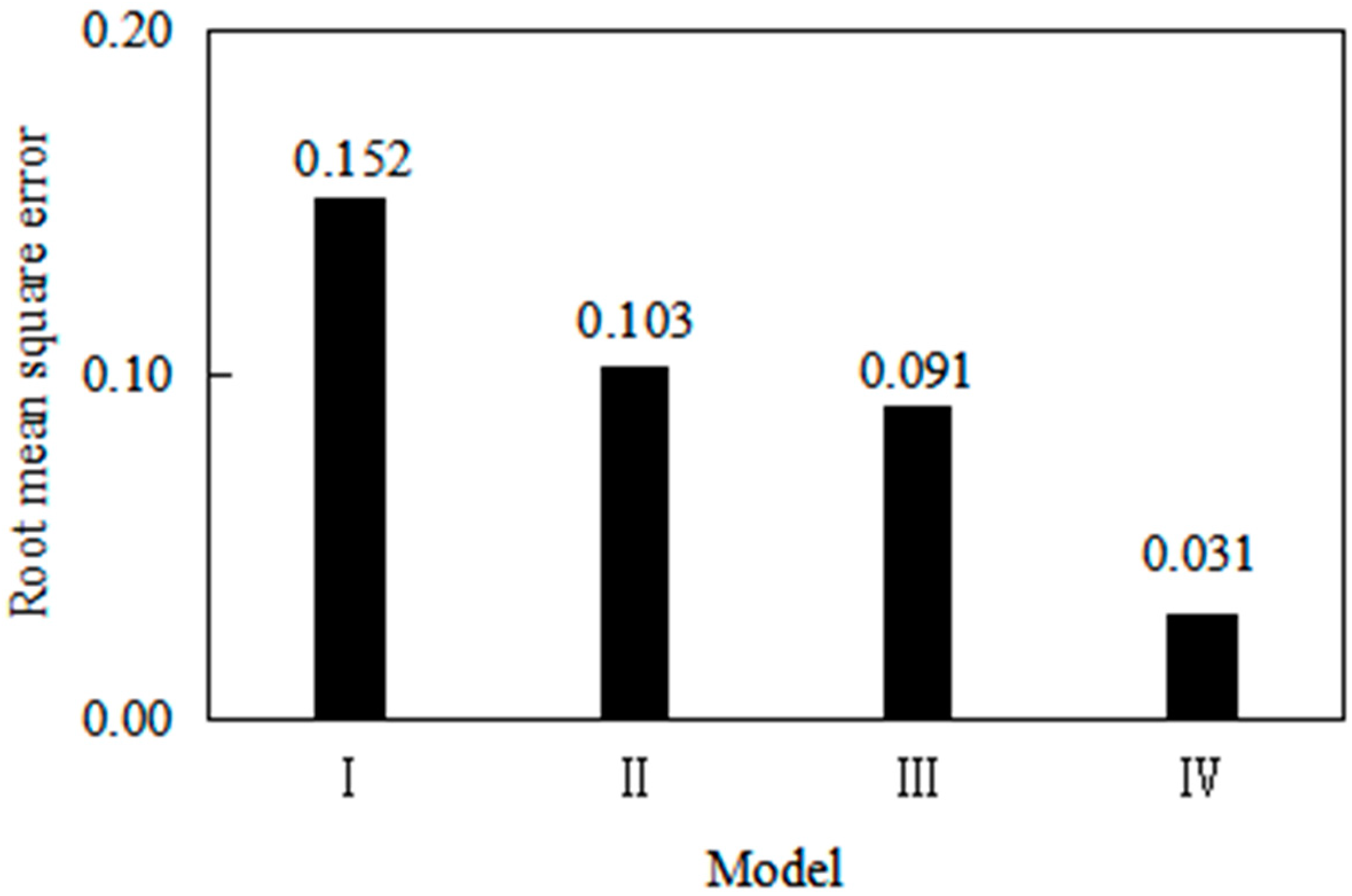
Based on the above calculation results, the average relative errors and root mean square errors of the prediction results were further obtained, as shown in Figure 3 and Figure 4.
It can be seen from Figure 3 and Figure 4 that the average relative error and root mean square error of the traditional gray model are 10.575% and 0.152, respectively. Therefore, its prediction accuracy is still relatively poor. After adopting translation transformation (model II), the smoothness of the original data sequence is improved, which helps to improve the prediction accuracy of model I. For the optimal weighted combination model, the prediction accuracy is still the highest, and its average relative error and root mean square error are only 2.143% and 0.031, respectively. In addition, the logarithmic function model also has good prediction accuracy, followed by model II and model I.
Based on the above results, it can be seen that the optimal weighted combination model has higher fitting and prediction accuracy under different numbers of modeling samples, so the model is effective in predicting wax deposition thickness.
5. Conclusions
- (1)
- Based on the modeling characteristics of the traditional GM (1,1), an improved GM (1,1) based on translation transformation was proposed, and the effectiveness of the improved model was verified. The results showed that the average relative error of the improved model is always lower than that of the traditional model when the number of modeling samples is different. Therefore, translation transformation method can improve the accuracy of the traditional model and broaden the application range of the gray model.
- (2)
- Based on the traditional GM (1,1) and the logarithmic function model, a new combination model was proposed, and the weight coefficient of each single model was obtained by using the optimal weighting method. The calculation results of different modeling samples showed that the optimal weighted combination model has higher fitting accuracy and prediction accuracy than the traditional model and logarithmic function model, which can be used to predict the wax deposition thickness.
- (3)
- The improved GM (1,1) and the optimal weighted combination model that are proposed in this paper provide new ideas for predicting wax deposition. In the application process, the optimal weighted combination model only needs to determine the weight coefficient of each single model, so it has the characteristic of convenient application.
Author Contributions
Methodology, W.J., Q.Q., K.D. and Z.R.; investigation, W.J., K.D. and J.G.; writing—original draft, W.J.; writing—review and editing, Q.Q. All authors have read and agreed to the published version of the manuscript.
Funding
The authors gratefully acknowledge the financial support provided by the Natural Science Basic Research Program of Shaanxi Province (No. 2019JQ-811, Department of science and technology of Shaanxi Province), the Natural Science Basic Research Program of Shaanxi Province (No. 2023-JC-QN-0467, Department of science and technology of Shaanxi Province), the Natural Science Basic Research Program of Shaanxi Province (No. 2023-JC-YB-414, Department of science and technology of Shaanxi Province), and the Special Scientific Research Plan Projects of the Shaanxi Education Department (No. 20JK0844, Education Department of Shaanxi Provincial Government).
Data Availability Statement
Data are contained within the article.
Conflicts of Interest
Author K.D. was employed by the China Petroleum Engineering & Construction Southwest Company. The remaining authors declare that the research was conducted in the absence of any commercial or financial relationships that could be construed as a potential conflict of interest.
References
- Gan, Y.Y.; Chen, L.; Zhang, J.Q.; Betancourt, S.S.; Mullins, O.C.; Yan, Z.H.; Gao, X.F.; Tian, J.; Chen, W.H.; Wang, W.F. Wax-out cryo trapping; a new trap-filling process in fluid migration to oilfields. Energy Fuels 2022, 36, 8844–8852. [Google Scholar] [CrossRef]
- Lei, Y.; Wang, H.; Li, S.S.; Liu, X.Q.; Zhu, H.R.; Gao, Y.M.; Peng, H.P.; Yu, P.F. Effect of existence state of asphaltenes on the asphaltenes-wax interaction in wax deposition. Petrol. Sci. 2023, 20, 507–514. [Google Scholar] [CrossRef]
- Gabriel, S.; Nagu, D.; Cem, S. Dynamic microscopic study of wax deposition: Particulate deposition. Energy Fuels 2021, 35, 12065–12074. [Google Scholar]
- Yang, F.; Zhao, Y.S.; Sjöblom, J.; Li, C.X.; Paso, K.G. Polymeric wax inhibitors and pour point depressants for waxy crude oils: A critical review. J. Disper. Sci. Technol. 2014, 36, 213–225. [Google Scholar] [CrossRef]
- Singh, P.; Venkatesan, R.; Fogler, H.S. Formation and aging of incipient thin film wax oil gels. AIChE J. 2000, 46, 1059–1074. [Google Scholar] [CrossRef]
- Zhou, Y.X.; Gong, J.; Wang, P.Y. Modeling of wax deposition for water-in-oil dispersed flow. Asia-Pac. J. Chem. Eng. 2016, 11, 108–117. [Google Scholar] [CrossRef]
- Wang, P.Y.; Wang, W.; Gong, J.; Zhou, Y.X.; Yang, W.; Zhang, Y. Effect of pour point on wax deposition under static cooling conditions. Asia-Pac. J. Chem. Eng. 2013, 8, 749–755. [Google Scholar] [CrossRef]
- Masoudi, S.; Sefti, M.V.; Jafari, H.; Modares, H. The hardening process and morphology of a wax deposit in a pipe flow. Petrol. Sci. Technol. 2010, 28, 1598–1610. [Google Scholar] [CrossRef]
- Chi, Y.D.; Daraboina, N.; Sarica, C. Investigation of inhibitors efficacy in wax deposition mitigation using a laboratory scale flow loop. AIChE J. 2016, 62, 4131–4139. [Google Scholar] [CrossRef]
- Lu, Y.D.; Huang, Z.Y.; Hoffmann, R.; Amundsen, L.; Fogler, H.S. Counterintuitive effects of the oil flow rate on wax deposition. Energy Fuels 2012, 26, 4091–4097. [Google Scholar] [CrossRef]
- Hoffmann, R.; Amundsen, L. Single-phase wax deposition experiments. Energy Fuels 2010, 24, 1069–1080. [Google Scholar] [CrossRef]
- Singh, P.; Venkatesan, R.; Fogler, H.S.; Nagarajan, N.R. Morphological evolution of thick wax deposits during aging. AIChE J. 2001, 47, 6–18. [Google Scholar] [CrossRef]
- Deng, J.L. Control problems of grey systems. Syst. Control Lett. 1982, 1, 288–294. [Google Scholar]
- Guo, Q.W.; Guo, B.H.; Wang, Y.G.; Tian, S.X.; Chen, Y. A combined prediction model composed of the GM (1,1) model and the BP neural network for major road traffic accidents in China. Math. Probl. Eng. 2022, 2022, 8392759. [Google Scholar] [CrossRef]
- Zhang, X.Q.; Wu, X.L.; Xiao, Y.M.; Shi, J.W.; Zhao, Y.; Zhang, M.H. Application of improved seasonal GM (1,1) model based on HP filter for runoff prediction in Xiangjiang River. Environ. Sci. Pollut. Res. 2022, 29, 52806–52817. [Google Scholar] [CrossRef]
- Yao, H.; Zhang, Q.X.; Niu, G.Y.; Liu, H.; Yang, Y.X. Applying the GM (1,1) model to simulate and predict the ecological footprint values of Suzhou city, China. Environ. Dev. Sustain. 2021, 23, 11297–11309. [Google Scholar] [CrossRef]
- Li, Z.J.; Yang, Q.C.; Wang, L.C.; Martín, J.D. Application of RBFN network and GM (1,1) for groundwater level simulation. Appl. Water Sci. 2017, 7, 3345–3353. [Google Scholar] [CrossRef]
- Chen, S.W.; Li, Z.G.; Zhou, S.X. Application of non-equal interval GM(1,1) model in oil monitoring of internal combustion engine. J. Cent. South Univ. Technol. 2005, 12, 705–708. [Google Scholar] [CrossRef]
- Hu, Y.C. Energy demand forecasting using a novel remnant GM (1,1) model. Soft Comput. 2020, 24, 13903–13912. [Google Scholar] [CrossRef]
- Wu, M.; Qiu, S.J.; Liu, J.F.; Zhao, L. Prediction model based on the Grey Theory for tackling wax deposition in oil pipelines. J. Nat. Gas Chem. 2005, 14, 243–247. [Google Scholar]
- Cheng, M.L.; Shi, G.J. Improved methods for parameter estimation of gray model GM (1,1) based on new background value optimization and model application. Commun. Stat-Simul. Comput. 2022, 51, 647–669. [Google Scholar] [CrossRef]
- Jin, W.B.; Quan, Q.; Hui, X.Z.; Chen, J.H.; Qin, G.W. Prediction of wax deposition thickness on pipe wall by improved GM (1,1) model based on data transformation method. Petrol. Sci. Technol. 2022, 40, 1551–1566. [Google Scholar] [CrossRef]
- Deng, Y.H. Improved combination GM(1, 1)model and its application in distortion inspction. Appl. Mech. Mater. 2011, 1449, 229–232. [Google Scholar] [CrossRef]
- Zhao, L.; Xu, H.K.; Cheng, H.L. Road traffic accidents prediction based on optimal weighted combined model. Comput. Eng. Appl. 2013, 49, 11–15. [Google Scholar]
- Li, D.W.; Chen, J.B.; Qiu, M.L. Research on population development trend in Huizhou of China forecast based on optimal weighted combination method and fractional grey model. J. Math. 2021, 2021, 3320910. [Google Scholar] [CrossRef]
- Su, X. Research on Wax Deposition and Pigging Periods in Submarine Waxy Crude Oil Pipeline. Master’s Thesis, Southwest Petroleum University, Chengdu, China, 2015. [Google Scholar]
Figure 1.
Average relative error of prediction results for each model (based on 5–9 sets of data to establish models).
Figure 1.
Average relative error of prediction results for each model (based on 5–9 sets of data to establish models).
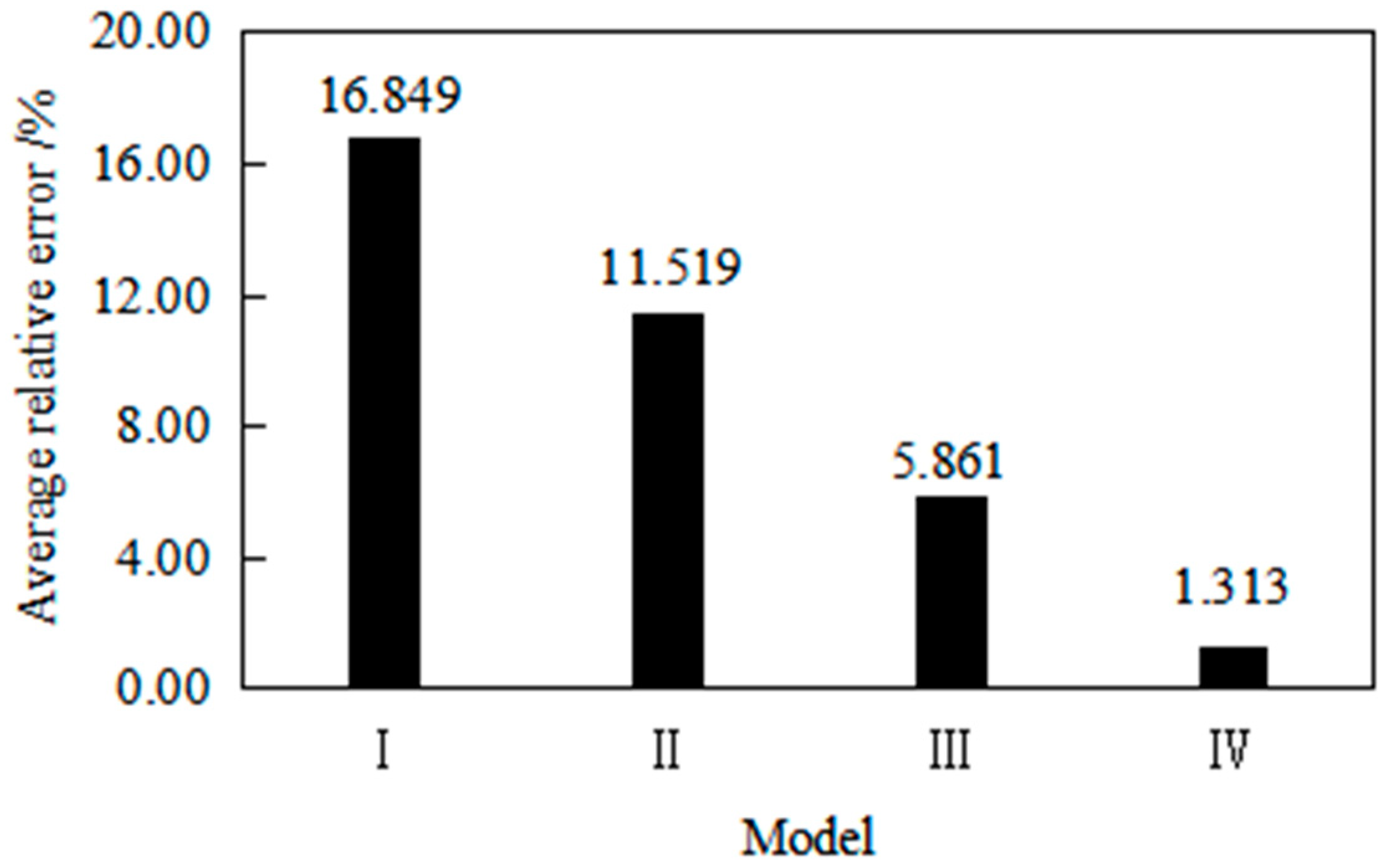
Figure 2.
Root mean square error of prediction results for each model (based on 5–9 sets of data to establish models).
Figure 2.
Root mean square error of prediction results for each model (based on 5–9 sets of data to establish models).
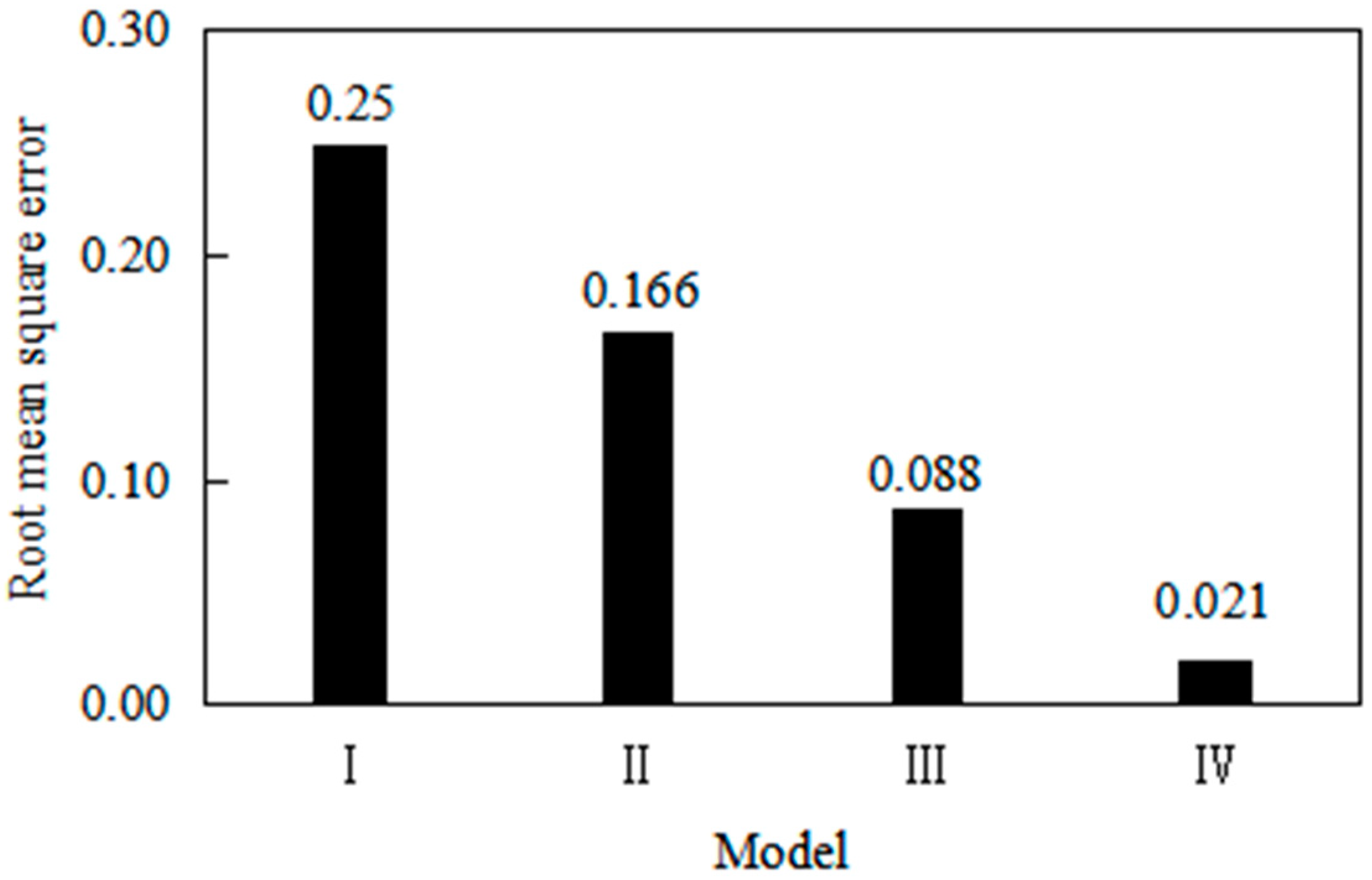
Figure 3.
Average relative error of prediction results for each model (based on 5–10 sets of data to establish models).
Figure 3.
Average relative error of prediction results for each model (based on 5–10 sets of data to establish models).
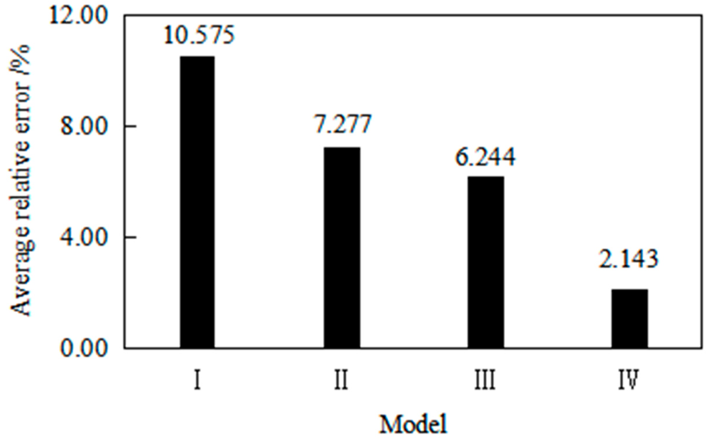
Figure 4.
Root mean square error of prediction results for each model (based on 5–10 sets of data to establish models).
Figure 4.
Root mean square error of prediction results for each model (based on 5–10 sets of data to establish models).

Table 1.
Indoor wax deposition experimental data.
| Time (h) | Thickness (mm) |
|---|---|
| 1 | 0 |
| 2 | 0 |
| 3 | 0 |
| 4 | 0 |
| 5 | 0.33 |
| 6 | 0.65 |
| 7 | 0.82 |
| 8 | 0.97 |
| 9 | 1.08 |
| 10 | 1.19 |
| 11 | 1.3 |
| 12 | 1.42 |
Table 2.
Calculation results and relative errors of each model (based on 5–9 sets of data to establish models).
Table 2.
Calculation results and relative errors of each model (based on 5–9 sets of data to establish models).
| Num | Test Value (mm) | Model I | Model II | Model III | Model IV | ||||
|---|---|---|---|---|---|---|---|---|---|
| Calculated Value (mm) | Relative Error (%) | Calculated Value (mm) | Relative Error (%) | Calculated Value (mm) | Relative Error (%) | Calculated Value (mm) | Relative Error (%) | ||
| 5 | 0.33 | 0.33 | 0.000 | 0.33 | 0.000 | 0.3267 | 1.000 | 0.3274 | 0.788 |
| 6 | 0.65 | 0.6794 | 4.523 | 0.6715 | 3.308 | 0.6476 | 0.369 | 0.6540 | 0.615 |
| 7 | 0.82 | 0.7977 | 2.720 | 0.8018 | 2.220 | 0.8354 | 1.878 | 0.8278 | 0.951 |
| 8 | 0.97 | 0.9367 | 3.433 | 0.9438 | 2.701 | 0.9686 | 0.144 | 0.9622 | 0.804 |
| 9 | 1.08 | 1.0998 | 1.833 | 1.0987 | 1.731 | 1.0719 | 0.750 | 1.0775 | 0.231 |
| 10 | 1.19 | 1.2914 | 8.521 | 1.2676 | 6.521 | 1.1563 | 2.832 | 1.1834 | 0.555 |
| 11 | 1.3 | 1.5163 | 16.638 | 1.4517 | 11.669 | 1.2277 | 5.562 | 1.2855 | 1.115 |
| 12 | 1.42 | 1.7805 | 25.387 | 1.6524 | 16.366 | 1.2895 | 9.190 | 1.3878 | 2.268 |
Table 3.
Average relative error of fitting results for each model (based on 5–9 sets of data to establish models).
Table 3.
Average relative error of fitting results for each model (based on 5–9 sets of data to establish models).
| Model | Average Relative Error (%) |
|---|---|
| Model I | 2.502 |
| Model II | 1.992 |
| Model III | 0.828 |
| Model IV | 0.678 |
Table 4.
Calculation results and relative errors of each model (based on 5–10 sets of data to establish models).
Table 4.
Calculation results and relative errors of each model (based on 5–10 sets of data to establish models).
| Num | Test Value (mm) | Model I | Model II | Model III | Model IV | ||||
|---|---|---|---|---|---|---|---|---|---|
| Calculated Value (mm) | Relative Error (%) | Calculated Value (mm) | Relative Error (%) | Calculated Value (mm) | Relative Error (%) | Calculated Value (mm) | Relative Error (%) | ||
| 5 | 0.33 | 0.33 | 0.000 | 0.33 | 0.000 | 0.3206 | 2.848 | 0.3229 | 2.152 |
| 6 | 0.65 | 0.6996 | 7.631 | 0.6866 | 5.631 | 0.6489 | 0.169 | 0.6613 | 1.738 |
| 7 | 0.82 | 0.8038 | 1.976 | 0.8045 | 1.890 | 0.8410 | 2.561 | 0.8319 | 1.451 |
| 8 | 0.97 | 0.9236 | 4.784 | 0.9315 | 3.969 | 0.9773 | 0.753 | 0.9642 | 0.598 |
| 9 | 1.08 | 1.0612 | 1.741 | 1.0683 | 1.083 | 1.0830 | 0.278 | 1.0777 | 0.213 |
| 10 | 1.19 | 1.2194 | 2.471 | 1.2156 | 2.151 | 1.1694 | 1.731 | 1.1816 | 0.706 |
| 11 | 1.3 | 1.4011 | 7.777 | 1.3744 | 5.723 | 1.2424 | 4.431 | 1.2811 | 1.454 |
| 12 | 1.42 | 1.6099 | 13.373 | 1.5454 | 8.831 | 1.3056 | 8.056 | 1.3798 | 2.831 |
Table 5.
Average relative error of fitting results for each model (based on 5–10 sets of data to establish models).
Table 5.
Average relative error of fitting results for each model (based on 5–10 sets of data to establish models).
| Model | Average Relative Error (%) |
|---|---|
| Model I | 3.101 |
| Model II | 2.454 |
| Model III | 1.390 |
| Model IV | 1.143 |
Disclaimer/Publisher’s Note: The statements, opinions and data contained in all publications are solely those of the individual author(s) and contributor(s) and not of MDPI and/or the editor(s). MDPI and/or the editor(s) disclaim responsibility for any injury to people or property resulting from any ideas, methods, instructions or products referred to in the content. |
© 2023 by the authors. Licensee MDPI, Basel, Switzerland. This article is an open access article distributed under the terms and conditions of the Creative Commons Attribution (CC BY) license (https://creativecommons.org/licenses/by/4.0/).
Share and Cite
MDPI and ACS Style
Jin, W.; Quan, Q.; Dai, K.; Ren, Z.; Guan, J. Research on the Prediction of Wax Deposition Thickness on Pipe Walls Based on the Optimal Weighted Combination Model. Processes 2023, 11, 3363. https://doi.org/10.3390/pr11123363
AMA Style
Jin W, Quan Q, Dai K, Ren Z, Guan J. Research on the Prediction of Wax Deposition Thickness on Pipe Walls Based on the Optimal Weighted Combination Model. Processes. 2023; 11(12):3363. https://doi.org/10.3390/pr11123363
Chicago/Turabian StyleJin, Wenbo, Qing Quan, Kemin Dai, Zongxiao Ren, and Jing Guan. 2023. "Research on the Prediction of Wax Deposition Thickness on Pipe Walls Based on the Optimal Weighted Combination Model" Processes 11, no. 12: 3363. https://doi.org/10.3390/pr11123363
Note that from the first issue of 2016, this journal uses article numbers instead of page numbers. See further details here.