Next Article in Journal
Determination of Sesquiterpenes in Wines by HS-SPME Coupled with GC-MS
Next Article in Special Issue
Fractionation and Characterization of High Aspect Ratio Gold Nanorods Using Asymmetric-Flow Field Flow Fractionation and Single Particle Inductively Coupled Plasma Mass Spectrometry
Previous Article in Journal
Automated Analysis of Oxytocin by On-Line in-Tube Solid-Phase Microextraction Coupled with Liquid Chromatography-Tandem Mass Spectrometry
 
 
Please note that, as of 1 January 2016, Chromatography has been renamed to Separations and is now published here.
Article

Adverse-Mode FFF: Multi-Force Ideal Retention Theory

1
The Rudolf Peierls Centre for Theoretical Physics, 1 Keble Road, Oxford OX1 3NP, UK
2
Department of Physics, University of Ottawa, 150 Louis-Pasteur, Ottawa, ON K1N 6N5, Canada
*
Author to whom correspondence should be addressed.
Chromatography 2015, 2(3), 392-409; https://doi.org/10.3390/chromatography2030392
Submission received: 31 May 2015 / Revised: 25 June 2015 / Accepted: 29 June 2015 / Published: 7 July 2015
(This article belongs to the Special Issue Field-Flow Fractionation)

Abstract

:
A novel field-flow fractionation (FFF) technique, in which two opposing external forces act on the solute particles, is proposed. When the two external forces are sufficiently strong and scale differently as a function of the solutes’ property of interest (such as the solute particle size), a sharp peak in the retention ratio (dramatic drop in elution time) is predicted to exist. Because the external forces oppose one another, we refer to this novel technique as adverse-mode FFF. The location of this peak is theoretically predicted and its ideal width estimated. The peak can become quite sharp by simultaneously increasing the strength of both fields, suggesting that adverse-mode FFF could be a useful technique for accurately measuring single species solute size.

1. Introduction

Field-flow fractionation (FFF) is an elegant separation technique. Species separation can occur by applying an external field perpendicular to a non-uniform, laminar flow profile that carries a mixture of different solute species along a channel. The perpendicular field concentrates the solutes against one of the channel walls (the accumulation wall), while diffusivity resists the inhomogeneity. The competition between thermal energy and the potential energy drop results in an exponential concentration distribution near equilibrium for each of the solutes. If the force acting on each species differs due to differing properties of interest, such as solute size, then the range of the exponential distributions vary, as well. Solute particles that reside on average nearer the channel wall are carried with a slower average speed than samples with a larger mean height. This is ideal normal-mode FFF.
Normal-mode FFF has proven to be a widely successful separation technique [1,2,3,4,5,6,7]. Recent applications of FFF include natural and artificial nanoparticles in environmental samples [8,9,10], protein aggregates [11], drug delivery nanocarriers [12], subcellular organelles [13], food applications [14], quantum dots [15], red blood cells [16], and many more. FFF has been applied to separate solutes as small as 1 nm [17,18,19,20] and as large as 0.1 mm [21,22]. The flexibility of FFF results from the large number of potential transverse external fields that can be used. Gravitational [23,24], centrifugal sedimentation [25,26], electrical [27,28], magnetic [29,30], dielectrophoretic [31,32], acoustic [33,34], photophoretic [35,36], cross-flow (both symmetrical [37,38] and asymmetrical [39,40]) and thermal [41,42] fields have all been utilized by FFF. Cross-flows (both symmetrical and asymmetrical), sedimentation and thermal gradients are the most commonly-employed fields. However, electrical, pressure, magnetic, dielectrophoretic, acoustic and photophoretic fields have been demonstrated as acceptable [43,44]. Ideal normal-mode retention theory often suffices for this disparate family of fields and samples [43,44,45,46,47]. However, complications often arise.
Most complications negatively impact separation [48]. Such complications may include flow profile distortion by the external field [43,49,50], hydrodynamic interactions leading to wall-induced lag [51,52], finite-aspect ratio channels [53], slip [54] and concentration effects [55]. On the other hand, a minority of complications may be beneficial to separation. For instance, steric-interactions with the accumulation wall lead to steric-mode FFF, and lift-based hyperlayer FFF results from non-trivial hydrodynamic forces between the accumulation wall and the solutes [48].
Multiple external fields acting simultaneously on the solutes are commonly considered a negative complication if the strength of the force on each species is unknown, as could occur if samples possess large, but unsuspected mass difference. However, when engineered, multiple external fields acting in concert can be beneficial, as demonstrated by microfluidic thermal-electric FFF [56]. A similar method, combining electric-FFF and flow-FFF, was recently used to accurately determine the electrophoretic mobility of nanoparticles and proteins [57]. The prescribed and simultaneous application of two aligned external fields is termed additive-mode FFF [56]. Likewise, Kato and Nakamura have successfully developed a hyphenated flow-FFF and centrifugal-FFF apparatus, in which the two fields are applied in series [58].
The current manuscript considers a simple, though perhaps non-intuitive, variation on additive-mode FFF. Rather than applying two independent external forces in concert towards the accumulation wall, it is proposed that a pair of opposing forces with different scaling be applied to the sample (Figure 1). While the two forces do indeed compete (reducing the net force applied to the solutes at all points in the channel), the different scalings as a function of solute size allow there to be a predictable size at which the forces balance, producing a sharp increase in elution speed. We term this novel technique adverse-mode FFF.
Figure 1. Schematic of the concept behind adverse-mode field-flow fractionation (FFF). Two strong forces ( f 1 and f 2 ), which scale differently with solute size, oppose one another. At small sizes, the force with the smaller scaling (say α 1 ) dominates and the solute undergoes steric-mode at the accumulation (bottom) wall. At the specific size r ˜ L , the two forces are equal, and the solute is buoyant, such that it diffusively samples all sterically available flows equally. At larger sizes, the adverse force dominates, and the solute is pushed against the opposite (top) channel wall (what was previously the depletion wall).
Chromatography 02 00392 g001

2. Multi-Force Ideal Retention Theory

For specificity, assume that the external forces f i acting on the sample are each a function of solute size r. Generally speaking, if the net force is the sum of many fields ( f = f i = a i r α i ), then the retention parameter is:
λ = k B T h f = k B T h a i r α i
The retention parameter is an inverse Péclet number that describes the competition between the thermal energy k B T , which acts to disperse the solutes, and the drop in potential energy h f as the solute concentrates at the accumulation wall. The field coefficients a i can be positive or negative depending on the direction of the force. For a single external field, the retention parameter depends directly on solute size λ r - α 1 , and so, it is useful to define a device retention parameter [59], which characterizes the apparatus and is defined by λ Λ 1 r ˜ - α 1 , where · ˜ denotes non-dimensionalisation with channel height, h (e.g., r ˜ = r / h ).
The ideal concentration distribution of solutes as a function of distance from the accumulation wall y that results from the net force is:
n y ˜ = n 0 exp y ˜ r ˜ Γ for   r ˜ < y ˜ < 1 r ˜ 0 otherwise
where:
Γ r ˜ Λ i 1 r ˜ α i
and Λ i k B T / h 1 + α i a i . The zero in Equation (2) accounts for exclusion of the near wall region due to steric interactions with the walls, and n 0 is the concentration at the accumulation wall. The concentration in Equation (2) can be thought of as representing the probability distribution of particle heights y ˜ . The current study does not consider techniques in which external forces are a function of solute vertical position y ˜ , such as lift-based hyperlayer [48], acoustic [33,60] or dielectrophoretic levitation [61,62,63] FFF.

2.1. Retention Ratio of the Multi-Force Ideal Retention Theory

The average across the height of the elution channel of an arbitrary function is defined to be F = F n ¯ / n ¯ , where x ¯ = 1 h 0 h x d y . By Equation (2), the average height of the particles above the accumulation wall is then:
y ˜ = 1 Γ + 1 1 e 1 2 r ˜ Γ + r ˜ coth 1 2 r ˜ Γ 2
Using the average height with Poiseuille flow (with average fluid velocity u ¯ ) and a Faxén law correction for the finite size of the solutes [59], the average elution speed V of an eluting sample subject to multiple external forces can be found. This is most often described as the retention ratio R 1 V / u ¯ . The retention ratio is calculated to be:
R 1 = 6 1 2 r ˜ Γ L 1 2 r ˜ Γ 2 + 6 r ˜ 1 4 r ˜ 3
where L x = coth x 1 / x is the Langevin function. The average height and the retention ratio both have identical forms to the single force equations, except that Γ = Λ i 1 r ˜ α i replaces Λ 1 r ˜ α . Equation (5) is the FFF retention ratio for a system in which multiple forces that scale simply with particle size act on the sample.

2.2. Higher Moments of the Multi-Force Ideal Retention Theory

The retention ratio given by Equation (5) represents the ideal first moment of the elution velocity distribution. Much work has been done to theoretically tackle the dispersion of elution bands in FFF [64,65]. Such work is generally concerned with plate height, which accounts for band spreading of sample peaks by thermal diffusion, advection and non-equilibrium corrections to the concentration distribution. Here, diffusion is not considered. Only the ideal moments of the velocity distribution of a sample subject to multiple forces are derived. Additional dispersion is not considered analytically.
The fluid flow profile between two no-slip parallel plates is parabolic, and thus, the velocity of a solute particle at height y ˜ is V ˜ = V 6 u ¯ = y ˜ y ˜ 2 r ˜ 2 / 3 , where the last term accounts for the Faxén correction. The j-th moment is:
R j = n V ˜ j n
Higher moments involve many coefficients due to the parabolic profile of the flowing carrier fluid. These myriad coefficients are cumbersome, and so, a general and relatively convenient framework for calculating the moments is desirable. The functions being averaged are polynomials in y ˜ with coefficients c i , which may be functions of solute size r ˜ :
V ˜ 6 = r ˜ 2 3 + y ˜ y ˜ 2 = c 0 + c 1 y ˜ + c 2 y ˜ 2
V ˜ 2 6 2 = r ˜ 4 9 2 r ˜ 2 3 y ˜ + 1 + 2 r ˜ 2 3 y ˜ 2 2 y ˜ 3 + y ˜ 4 = c 0 + c 1 y ˜ + c 2 y ˜ 2 + c 3 y ˜ 3 + c 4 y ˜ 4
V ˜ 3 6 3 = r ˜ 6 27 + r ˜ 4 3 y ˜ r ˜ 2 1 + r ˜ 2 3 y ˜ 2 + 1 + 2 r ˜ 2 2 y ˜ 3 3 + r ˜ 2 y ˜ 4 + 3 y ˜ 5 y ˜ 6 = c 0 + c 1 y ˜ + c 2 y ˜ 2 + c 3 y ˜ 3 + c 4 y ˜ 4 + c 3 y ˜ 5 + c 4 y ˜ 6
and so on. It is apparent that each moment is a sum of integrals of each term in these polynomials, which necessarily have the form Θ j r ˜ 1 r ˜ e y ˜ r ˜ Γ y ˜ j d y ˜ . For all j, this integral has an analytical solution of the form Θ j X j e 2 r ˜ 1 Γ + Y j / Γ j + 1 , where X j and Y j can be identified from each integral. Defining r * = r ˜ 1 for brevity, the first many are:
X 0 = 1 X 1 = Γ r * 1 X 2 = Γ r * Γ r * 2 + 2 X 3 = Γ r * Γ r * Γ r * 3 + 6 6 X 4 = Γ r * Γ r * Γ r * Γ r * 4 + 12 24 + 24 X 5 = Γ r * Γ r * Γ r * Γ r * Γ r * 5 + 20 60 + 120 120
Y 0 = 1 Y 1 = Γ r ˜ + 1 Y 2 = Γ r ˜ Γ r ˜ + 2 + 2 Y 3 = Γ r ˜ Γ r ˜ Γ r ˜ + 3 + 6 + 6 Y 4 = Γ r ˜ Γ r ˜ Γ r ˜ Γ r ˜ + 4 + 12 + 24 + 24 Y 5 = Γ r ˜ Γ r ˜ Γ r ˜ Γ r ˜ Γ r ˜ + 5 + 20 + 60 + 120 + 120
and so on. From these functions, the j th moment of the solute velocity can be written as:
R j = n V ˜ j n = 6 j i = 0 2 j c i Θ i Γ 1 e 2 r ˜ 1 Γ
where the coefficients come from the appropriate polynomial in Equations (7)-(9). More conveniently, all moments can be written in the explicitly analytical form commonly used for the ideal retention ratio:
R j = A j L γ + B j
A j = 6 j 2 C X , j + C Y , j
B j = 6 j 2 C X , j 1 γ 1 + C Y , j 1 γ + 1
C X , j = i = 0 2 j c i X i Γ i ; C Y , j = i = 0 2 j c i Y i Γ i
γ = Γ 2 1 2 r ˜
The ideal moments of FFF for any number of external fields is given analytically by Equation (11). The ideal moments of traditional FFF with only a single external field are trivially obtained from Equation (11) by simply setting Γ = Λ 1 r ˜ α .
Let us use Equation (11) to calculate the first three moments of velocity as a function of the multi-field device retention parameter Γ and solute size r ˜ . The first moment is the retention ratio, which is given by:
A 1 = 6 1 2 r ˜ Γ
B 1 = 2 r ˜ 3 4 r ˜
and Equation (11), which clearly agrees with Equation (5). An example for a single external field defined by Λ 1 = 10 5 and α 1 = 3 is shown in Figure 2. The analytical form agrees with the numerical form as determined by numerically-integrating the probability distribution of particle heights through n y ˜ or the probability distribution of velocities p V V .
Figure 2. First three cumulants of the velocity distribution for a single external field characterized by Λ 1 = 10 5 and α 1 = 3 as a function of solute size. The functions are determined analytically via Equation (11). The mean (retention ratio) is given by Equations (16)-(17), the variance by Equations (18)-(19) and the skewness by Equations (20)-(21).
Chromatography 02 00392 g002
The second moment is given by:
A 2 = 24 1 2 r ˜ Γ r ˜ 3 4 r ˜ 18 Γ 2
B 2 = 4 r ˜ 2 3 4 r ˜ 2 + 18 1 2 r ˜ 2 Γ 2
The related second cumulant is the variance of the velocity distribution, σ 2 = R 2 R 1 2 . The variance for a single external field Λ 1 = 10 5 and α 1 = 3 is shown in Figure 2. It should be recalled that this is the ideal variance, which does not take into account thermal diffusion or non-equilibrium effects [64,65]. To first order, additional dispersion could be superimposed on σ 2 . The ideal variance goes to zero when the solutes are nearly entirely in steric contact with the accumulation wall.
The third moment is given by:
A 3 = 72 1 2 r ˜ Γ r ˜ 2 3 4 r ˜ 2 + 18 Γ 2 1 10 r ˜ + 12 r ˜ 2 1080 Γ 4
B 3 = 8 r ˜ 3 3 4 r ˜ 3 + 54 r ˜ Γ 2 1 2 r ˜ 2 3 4 r ˜ 1620 Γ 4 1 2 r ˜ 2
The third moment R 3 is related to the skewness κ = R 3 3 R 2 R 1 + 2 R 1 3 . The skewness for a single external field Λ 1 = 10 5 and α 1 = 3 is shown in Figure 2. Both positive and negative skewness are observed. The analytical form for the skewness agrees with the numerically-determined forms from the probability distribution of particle heights and the probability distribution of velocities.
Although Equation (11) gives all of the moments of the distribution in a convenient form, it is also possible to find the ideal distribution of the velocities p V V by inverting Equation (7) to find the height as a function of velocity y ˜ = 1 2 1 ± 1 4 3 r ˜ 2 2 3 V ˜ where the + and − signs refer to heights above and below the centreline, respectively. The minimum particle velocity occurs when the particle is in contact with either wall:
V ˜ min = V ˜ r ˜ = V ˜ 1 r ˜ = 6 r ˜ 1 4 r ˜ / 3
and the maximum is at the centreline
V ˜ max = V ˜ 1 / 2 = 3 2 1 4 r ˜ 2 / 3
These functions are sufficient to write the average of an arbitrary function in terms of an integral over the velocity and demanding the condition that p V d V = 1 gives the full probability distribution of velocities to be:
p V = Γ 6 cosh Γ 2 1 4 3 r ˜ 2 2 3 V ˜ csch 1 2 r ˜ Γ 2 9 12 r ˜ 2 6 V ˜ 1 / 2 V ˜ min V ˜ V ˜ max 0 otherwise
The velocity probability distribution provides an additional method to determine any average via F = p V F V d V . In particular, the moments of the velocity distribution (including the first moment, which is the retention ratio) can be found. Doing so numerically verifies the analytical forms given by Equation (11), as seen in Figure 2.
Having constructed a general ideal retention theory for an FFF system subject to multiple forces, this paper now turns to the proposed technique of adverse-FFF, in which a pair of strong ( Λ i 1 ), opposing forces with different scalings ( α 1 α 2 ) are applied to the eluting sample.

3. Adverse-Mode FFF: Benefit of Two Opposing Forces

Consider a pair of opposing forces with different scaling exponents α 1 and α 2 acting on a particle (Figure 1). At small solute sizes, the force with the lower α (say α 1 ) dominates and pushes the solute distribution against the accumulation wall where the carrier velocity is small, but as the size grows, the opposing force becomes stronger. At a given size r ˜ L , the two forces exactly balance, and the net force is zero. As the size (and therefore, force) is increased further, the particle is pushed against the upper wall (formerly the depletion wall), and the system has effectively flipped. In a manner of speaking, this situation effectively generates a second normal-mode regime, but at larger solute sizes (and therefore, stronger forces).
It is expected that the solutes will usually elute in steric-mode FFF and will be carried by the slow moving near-wall fluid velocity, except when the two forces balance. When the forces exactly cancel, the particle is buoyant and not confined to either wall. The average velocity is fastest at that specific size r ˜ L , for which the solute elutes as in hydrodynamic chromatography, diffusively sampling all sterically available flow velocities with equal probability. Thus, a peak in the retention ratio as a function of size occurs where the opposing forces balance. When both of the opposing external fields are strong, the retention ratio peak can be quite sharp, as we shall demonstrate.

3.1. Adverse-Mode: Retention Ratio Peak

Such peaks can be seen in Figure 3 for a pair of moderate, opposing fields as calculated from Equation (5). The full ideal retention curves are shown, including the Faxén-mode size regime [59]. The solid black curve shows the retention ratio curve for a single external field ( Λ 2 = 0 ) with device retention parameter Λ 1 = 10 3 and α 1 = 1 . This curve is qualitatively similar to the curve in Figure 2. When an opposing field with α 2 = 3 competes with the principle external field, a steep peak arises. Because of the solutes’ finite size, the maximum peak height is even greater than R 1 = 1 , which is the retention ratio of tracer particles, and this increase occurs over a relatively narrow range of solute sizes. In Figure 3, the scalings α 1 = 1 and α 2 = 3 are used for all curves.
The position of the peak maxima in Figure 3 can be simply predicted to be the point at which the forces balance ( i Λ i 1 r ˜ L α i = 0 ). For a pair of opposing external fields, this occurs at the solute size:
r ˜ L = Λ 1 Λ 2 1 / α 1 α 2
As can be seen in Figure 3, Equation (25) accurately predicts the ideal peak position for adverse-mode FFF. Keeping the ratio of Λ 1 / Λ 2 constant fixes the peak position r ˜ L .
The scalings α 1 = 1 and α 2 = 3 used above are physically motivated, as they belong to experimentally-demonstrated sub-techniques of FFF. Flow-FFF [37,39,66,67], thermal-FFF [41,68,69] and electrical-FFF [27,70,71] each have a force that scales as α i = 1 , while sedimentation-FFF [25,72] (including gravitational-FFF [23,73]) is the most obvious commonly-used technique with α i = 3 . External forces with scaling of α i = 2 are not commonly utilized by FFF apparatuses. We stress again that adverse-FFF requires two forces with differing scalings as a function of solute size and that the forces balance at all points in the channel when the solute size is r ˜ L . In this way, adverse-FFF differs from lift-based hyperlayer [48], acoustic [33,60] or dielectrophoretic levitation [61,62,63] FFF, in which there are specific equilibrium heights within the channel at which forces balance. Such techniques tend to focus the solutes towards these points, which is not the case in adverse-FFF.
Figure 3. Retention ratio as a function of solute size for two constant opposing fields (adverse-mode FFF). Moderate opposing fields are shown. The force toward one wall scales as α 1 = 1 (as in flow-FFF), while the other scales as α 2 = 3 (sedimentation-like fields). Solid lines show the full theory (Equation (5)), while dashed lines show the near-peak approximation (Equation (26)). Dots mark r ˜ L from Equation (25).
Chromatography 02 00392 g003

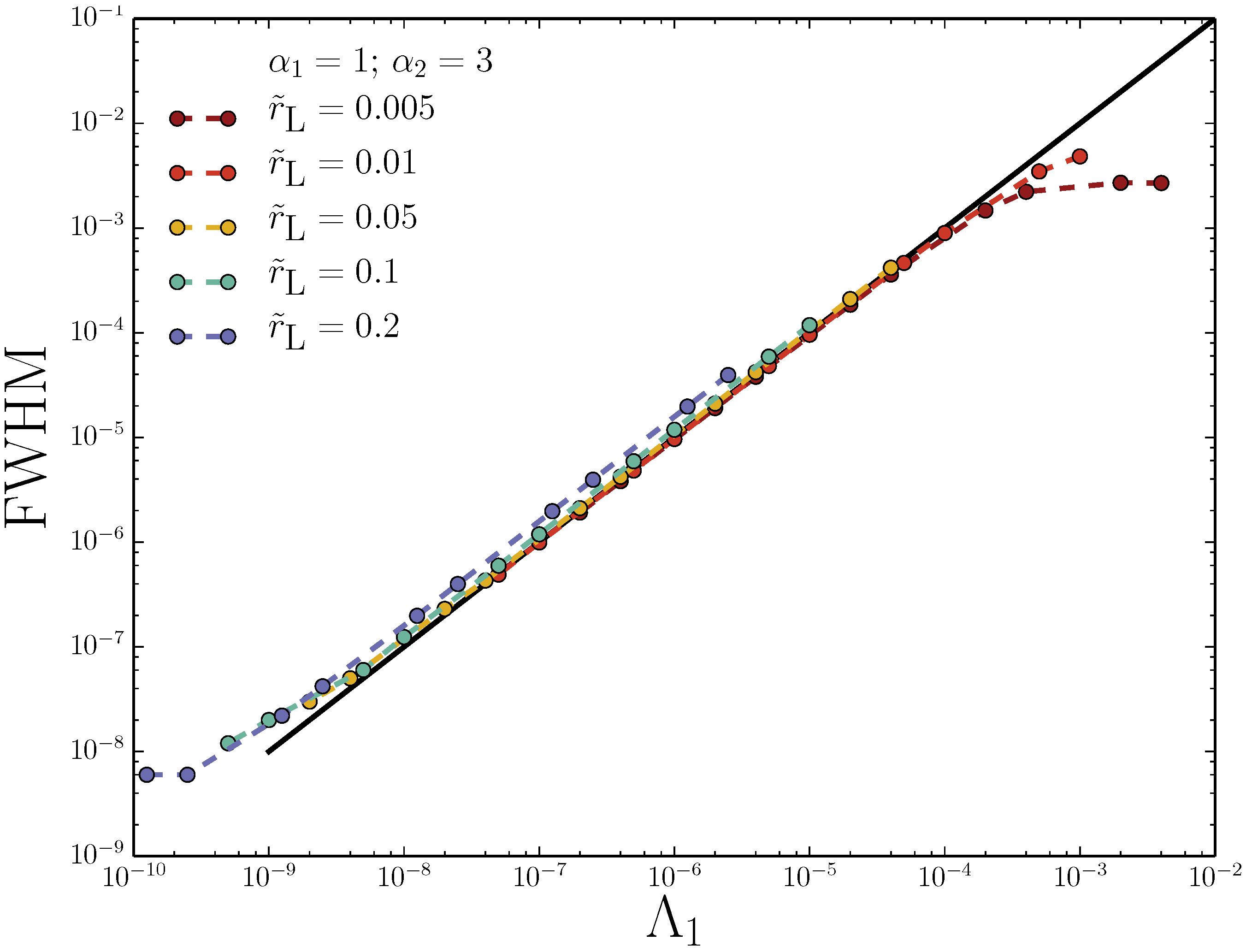
3.2. Adverse-Mode: Retention Ratio Peak Width

By increasing the field strengths (decreasing the two Λ i values), the adverse-FFF peaks narrow significantly (Figure 4). The change in R 1 near the peak is large, while the steric-mode FFF occurs as a slowly varying background retention ratio over the width of the peak. Therefore, two samples of similar size elute with very similar retention times if they have sizes that both fall in the steric-mode background. Only if one of the two samples has a size that corresponds to the narrow peak position while the other does not would they have substantially different retention times.
Near r ˜ L , the retention ratio peak can be simply approximated by expanding Equation (5) about Γ 0 , which produces the approximation:
R 1 1 + 2 r ˜ 4 r ˜ 2 1 2 r ˜ 4 60 Γ 2
Considering Figure 3 and Figure 4, it can be seen that Equation (26) does a reasonable job approximating the peak height and width near the maximum. The maximum can be simply and accurately calculated by substituting r ˜ L into Equation (26). Unfortunately, this near-peak approximation fails to capture the long tails. While it might be possible to use Equation (26) to estimate the width of the peaks in a reasonable, but ultimately arbitrary, manner (such as by setting Equation (26) equal to zero and solving for r ˜ ), it is simplest to measure the full-width at half-maximum (FWHM) of those peaks by subtracting the Λ 2 = curve (solid black line) off of the adverse-FFF retention ratios curves. Narrowing the peak while keeping r ˜ L fixed requires that both fields are increased simultaneously. Figure 5 plots the FWHM against Λ 1 for a variety of fixed values of r ˜ L .
Figure 4. Same as Figure 3, but stronger opposing fields are applied.
Chromatography 02 00392 g004
Figure 5. Full-width half-maximum (FWHM) of peaks as a function of Λ 1 (field strength) for fixed values of peak position r ˜ L . FWHM is non-dimensionalized by channel height. The opposing field Λ 2 is set by Equation (25) for fixed r ˜ L .
Chromatography 02 00392 g005
Peak position is inconsequential to the narrowing of the adverse-FFF peak: simultaneously decreasing Λ 1 and Λ 2 narrows the peak in the same way for all r ˜ L , as seen in Figure 5. The curves are linear with a slope of one on the log-log graph, which demonstrates that simultaneously doubling both fields leaves the peak position unchanged, but halves the FWHM.

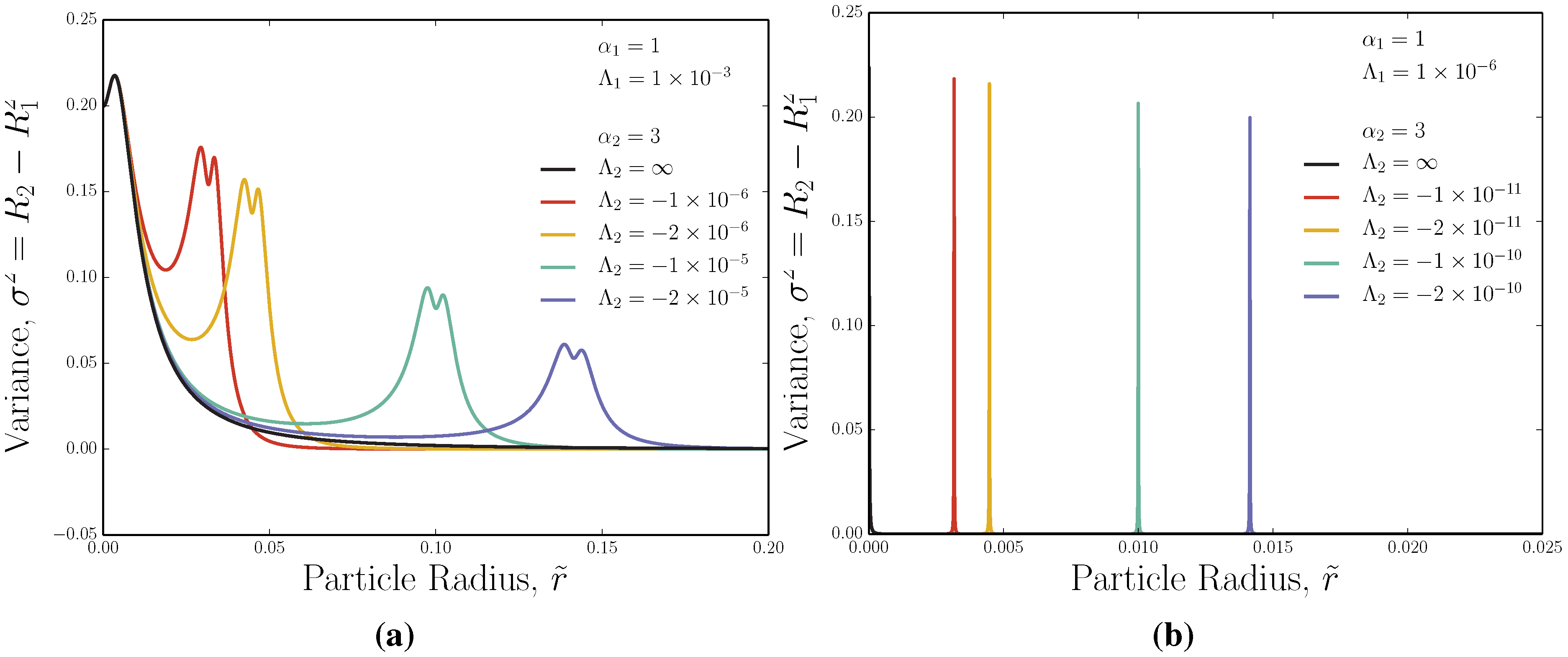
3.3. Adverse-Mode: Ideal Variance Peak

Thus far, only the adverse-FFF peak in the retention ratio has been considered. However, Equation (11) allows higher moments to be found. Equations (18)-(19) predict a sudden rise in the ideal (non-diffusive) variance of adverse-FFF (Figure 6).
Figure 6. Ideal variance as a function of solute size for adverse-FFF. (a) Moderate opposing fields; (b) strong opposing fields.
Chromatography 02 00392 g006
The peaks in variance are non-trivial. They are bimodal with a small local minimum occurring at the buoyancy point r ˜ L (Figure 6a). This is because of the symmetry of the Poiseuille flow about the centreline of the channel: just below or above r ˜ L , the majority of the solute particles sample a velocity profile that increases as a particle moves away from the wall, but once a substantial portion of the concentration passes the centreline, the particles sample the same velocities again, slightly decreasing the variance. When the strength of the opposing external fields Λ 1 and Λ 2 are large, as in Figure 6b, the peaks in variance narrow, and it becomes difficult to resolve their bimodal nature.

4. Implementation and Feasibility

The benefit of adverse-FFF would lie in two characteristics of the method:
  • The retention ratio peaks can be quite sharp for experimentally-achievable fields and;
  • the peak position r ˜ L can be simply predicted.
For these reasons, a system employing adverse-mode FFF could potentially be utilized to accurately measure the solute size of a single species. To measure an unknown solute size r ˜ , adverse-mode FFF might obey the following procedure:
  • Apply an external field with α 1 = 1 (such as flow-FFF, electrical-FFF or thermal-FFF) to an eluting sample. This field should have a small enough Λ 1 that elution occurs in the steric-mode regime of FFF.
  • Apply a field with α 2 = 3 and Λ 2 (such as centrifugal-FFF) to oppose the first field. Λ 2 must be smaller than Λ 1 for adverse-FFF to be successful.
  • Incrementally decrease Λ 2 from an initial large value, shifting r ˜ L to smaller values.
  • Identify the abrupt increase in retention ratio (plummet in retention time) when r ˜ L Λ 2 r ˜ .
  • Determine solute size through Equation (25).
  • Having found r ˜ L , simultaneously decrease the pair of device retention ratios Λ 1 and Λ 2 to hone the peak and improve the measurement accuracy.
The precision of the size measurement is limited by the maximum strength of the two opposing external fields. The essential requirement for adverse-FFF is implementing two opposing forces, which scale differently as a function of solute size and have controllable field strengths. One such device would be the separation system reported by Kato and Nakamura [58]. Although current operation is reportedly hyphenated, this system could conceivably be modified to operate in adverse-mode.
Let us now consider some approximate values for various FFF systems in order to assess the feasibility of adverse-FFF. Let the characteristic thermal energy be appropriate for room temperature, k B T 300 K, the viscosity be roughly that of water η 1 cP and the channel height be h 100 µm [43].
Since the two external forces must scale differently as a function of solute size, a sedimentation-FFF technique with α 2 = 3 is likely to be employed. This might be gravitational-FFF or centrifugal-FFF. For a centrifugal acceleration g = N G g 0 (with g 0 10 m · s 2 and N G the number of standard gravities) and a solute-carrier fluid density difference Δ ρ , the device retention ratio is Λ 2 = 3 k B T 4 π h 4 1 g Δ ρ . This would have a characteristic value of:
Λ 2 10 9 N G P
where 𝒫 is the percent difference of the solute to the carrier fluid density. The percent difference 𝒫 varies widely, but let us say P 5 % as appropriate for polystyrene [58] or polydimethylsiloxane [52]. Although N G = 1 for gravitational-FFF, it can be many thousands for centrifugal-FFF (say ∼10,000 [43]).
The opposing field should have α 1 < α 2 . There are many options for α 1 = 1 .
  • For thermal-FFF, Λ 1 10 4 K / Δ T , where Δ T 30 K is the temperature difference between the accumulation and depletion walls. This estimate assumes a characteristic Soret coefficient of ∼ 10 7 c m 2 s 1 K 1 [74].
  • For electrical-FFF, Λ 1 10 7 V / V eff , where V eff 0.1 V is the effective voltage between plates [75] and an electrophoretic mobility ∼ 10 4 c m 2 V 1 s 1 is assumed [56].
  • For flow-FFF, Λ 1 10 7 s 1 V 0 / V ˙ C , where the channel volume is V 0 10 6 m 3 and the cross-flow rate V ˙ C 1 mL/min [58].
In all of these cases, the adverse device retention parameter has an order of magnitude Λ 1 10 6 . Through Equation (25), the peak position is then predicted to occur at submicron scales, r L = h Λ 2 / Λ 1 1 / 2 0.1 µm.
These rough characteristic values of device retention parameters suggest that the adverse-FFF peak will be quite narrow (Figure 5), and so, solute sizes may be accurately determined using adverse-FFF. However, it also suggests a potential limitation of adverse-FFF. Nanoscopic values of r L demand that Λ 2 Λ 1 . For centrifugal-FFF, small values of Λ 2 may not be possible for small biological macromolecules, but only for dense nanoparticles, and require large rotor speeds. Of course, the opposing field strength can always be decreased (increase Λ 1 ) in order to shift r L towards nanoscopic values, but this compromises accuracy (Figure 5).

5. Conclusions

By applying two strongly-opposing external forces, which scale differently with solute size (or another physical characteristic of interest), a sharp peak occurs in the retention ratio and ideal variance curves. For solutes smaller than the peak position, the force that scales less strongly with size dominates, and the sample is concentrated near the accumulation wall. For larger solutes, the force that scales more strongly with size dominates, and the sample concentrates near what would normally be the depletion wall. The peak’s position can be accurately predicted as the size at which the opposing forces balance, and it commonly occurs in the size interval that would have traditionally been the steric-mode regime.
By increasing both of the opposing field strengths, the peak width can be sharpened and the background steric-mode retention ratio curve made flat. This sharp spike in retention ratio (or drop in elution time) at a well-predicted and potentially variable point suggests a method for accurately measuring submicron solute size. We propose that this technique be called adverse-mode FFF.

Acknowledgements

This work was funded through an EMBO-Long-Term Fellowship to Tyler N. Shendruk (ALTF181-2013) and an NSERCDiscovery Grant to Gary W. Slater.

Author Contributions

All authors contributed significantly to the reported work.

Conflicts of Interest

The authors declare no conflict of interest.

References

  1. Reschiglian, P.; Zattoni, A.; Roda, B.; Michelini, E.; Roda, A. Field-flow fractionation and biotechnology. Trends Biotechnol. 2005, 23, 475–483. [Google Scholar] [CrossRef] [PubMed]
  2. Kowalkowski, T.; Buszewski, B.; Cantado, C.; Dondi, F. Field-Flow Fractionation: Theory, Techniques, Applications and the Challenges. Crit. Rev. Anal. Chem. 2006, 36, 129–135. [Google Scholar] [CrossRef]
  3. Ratanathanawongs Williams, S.; Lee, D. Field-flow fractionation of proteins, polysaccharides, synthetic polymers, and supramolecular assemblies. J. Sep. Sci. 2006, 29, 1720–1732. [Google Scholar] [CrossRef]
  4. Roda, B.; Zattoni, A.; Reschiglian, P.; Moon, M.; Mirasoli, M.; Michelini, E.; Roda, A. Field-flow fractionation in bioanalysis: A review of recent trends. Anal. Chim. Acta 2009, 635, 132–143. [Google Scholar] [CrossRef] [PubMed]
  5. Qureshi, R.; Kok, W. Application of flow field-flow fractionation for the characterization of macromolecules of biological interest: A review. Anal. Bioanal. Chem. 2011, 399, 1401–1411. [Google Scholar] [CrossRef] [PubMed]
  6. Rambaldi, D.; Reschiglian, P.; Zattoni, A. Flow field-flow fractionation: Recent trends in protein analysis. Anal. Bioanal. Chem. 2011, 399, 1439–1447. [Google Scholar] [CrossRef] [PubMed]
  7. Runyon, J.R.; Ulmius, M.; Nilsson, L. A perspective on the characterization of colloids and macromolecules using asymmetrical flow field-flow fractionation. Colloids Surf. A: Physicochem. Eng. Asp. 2014, 442, 25–33. [Google Scholar] [CrossRef]
  8. Baalousha, M.; Stolpe, B.; Lead, J. Flow field-flow fractionation for the analysis and characterization of natural colloids and manufactured nanoparticles in environmental systems: A critical review. J. Chromatogr. A 2011, 1218, 4078–4103. [Google Scholar] [CrossRef] [PubMed]
  9. Stolpe, B.; Guo, L.; Shiller, A.M.; Aiken, G.R. Abundance, size distributions and trace-element binding of organic and iron-rich nanocolloids in Alaskan rivers, as revealed by field-flow fractionation and ICP-MS. Geochim. Cosmochim. Acta 2013, 105, 221–239. [Google Scholar] [CrossRef]
  10. Koopmans, G.; Hiemstra, T.; Regelink, I.; Molleman, B.; Comans, R. Asymmetric flow field-flow fractionation of manufactured silver nanoparticles spiked into soil solution. J. Chromatogr. A 2015, 1392, 100–109. [Google Scholar] [CrossRef] [PubMed]
  11. Tanase, M.; Zolla, V.; Clement, C.C.; Borghi, F.; Urbanska, A.M.; Rodriguez-Navarro, J.A.; Roda, B.; Zattoni, A.; Reschiglian, P.; Cuervo, A.M.; et al. Hydrodynamic size-based separation and characterization of protein aggregates from total cell lysates. Nat. Protoc. 2015, 10, 134–148. [Google Scholar] [CrossRef] [PubMed]
  12. Zattoni, A.; Roda, B.; Borghi, F.; Marassi, V.; Reschiglian, P. Flow field-flow fractionation for the analysis of nanoparticles used in drug delivery. J. Pharm. Biomed. Anal. 2014, 87, 53–61. [Google Scholar] [CrossRef] [PubMed]
  13. Yang, J.S.; Lee, J.Y.; Moon, M.H. High Speed Size Sorting of Subcellular Organelles by Flow Field-Flow Fractionation. Anal. Chem. 2015, 87, 6342–6348. [Google Scholar] [CrossRef] [PubMed]
  14. Nilsson, L. Separation and characterization of food macromolecules using field-flow fractionation: A review. Food Hydrocoll. 2013, 30, 1–11. [Google Scholar] [CrossRef]
  15. Moquin, A.; Neibert, K.D.; Maysinger, D.; Winnik, F.M. Quantum dot agglomerates in biological media and their characterization by asymmetrical flow field-flow fractionation. Eur. J. Pharm. Biopharm. 2015, 89, 290–299. [Google Scholar] [CrossRef] [PubMed]
  16. Moore, L.; Williams, P.; Nehl, F.; Abe, K.; Chalmers, J.; Zborowski, M. Feasibility study of red blood cell debulking by magnetic field-flow fractionation with step-programmed flow. Anal. Bioanal. Chem. 2014, 406, 1661–1670. [Google Scholar] [CrossRef] [PubMed]
  17. Rameshwar, T.; Samal, S.; Lee, S.; Kim, S.; Cho, J.; Kim, I. Determination of the Size of Water-Soluble Nanoparticles and Quantum Dots by Field-Flow Fractionation. J. Nanosci. Nanotechnol. 2006, 6, 2461–2467. [Google Scholar] [CrossRef] [PubMed]
  18. Stolpe, B.; Hassellöv, M. Changes in size distribution of fresh water nanoscale colloidal matter and associated elements on mixing with seawater. Geochim. Cosmochim. Acta 2007, 71, 3292–3301. [Google Scholar] [CrossRef]
  19. Von der Kammer, F.; Legros, S.; Hofmann, T.; Larsen, E.; Loeschner, K. Separation and characterization of nanoparticles in complex food and environmental samples by field-flow fractionation. TrAC Trends Anal. Chem. 2011, 30, 425–436. [Google Scholar] [CrossRef]
  20. Ratanathanawongs Williams, S.; Runyon, J.; Ashames, A. Field-Flow Fractionation: Addressing the Nano Challenge. Anal. Chem. 2011, 83, 634–642. [Google Scholar] [CrossRef] [PubMed]
  21. Giddings, J.; Myers, M. Steric Field-Flow Fractionation: A New Method for Separating 1 to 100 µm Particles. Sep. Sci. Technol. 1978, 13, 637–645. [Google Scholar] [CrossRef]
  22. Giddings, J.C.; Williams, P.S. Multifaceted analysis of 0.01 to 100 µm particles by sedimentation field-flow fractionation. Am. Lab. 1993, 95, 88–95. [Google Scholar]
  23. Berg, H.; Purcell, E.; Stewart, W. A method for separating according to mass a mixture of macromolecules or small particles suspended in a fluid. II. Experiments in a gravitational field. Proc. Natl. Acad. Sci. USA 1967, 58, 1286–1291. [Google Scholar] [CrossRef]
  24. Lee, S.; Kang, D.; Park, M.; Williams, P. Effect of Carrier Fluid Viscosity on Retention Time and Resolution in Gravitational Field-Flow Fractionation. Anal. Chem. 2011, 83, 3343–3351. [Google Scholar] [CrossRef] [PubMed]
  25. Berg, H.; Purcell, E. A method for separating according to mass a mixture of macromolecules or small particles suspended in a fluid. III. Experiments in a centrifugal fluid. Proc. Natl. Acad. Sci. USA 1967, 58, 1821–1828. [Google Scholar] [CrossRef]
  26. Mélin, C.; Perraud, A.; Akil, H.; Jauberteau, M.O.; Cardot, P.; Mathonnet, M.; Battu, S. Cancer Stem Cell Sorting from Colorectal Cancer Cell Lines by Sedimentation Field Flow Fractionation. Anal. Chem. 2012, 84, 1549–1556. [Google Scholar] [CrossRef] [PubMed]
  27. Caldwell, K.; Kesner, L.; Myers, M.; Giddings, J. Electrical Field-Flow Fractionation of Proteins. Science 1972, 176, 296–298. [Google Scholar] [CrossRef] [PubMed]
  28. Gigault, J.; Gale, B.; Le Hecho, I.; Lespes, G. Nanoparticle Characterization by Cyclical Electrical Field-Flow Fractionation. Anal. Chem. 2011, 83, 6565–6572. [Google Scholar] [CrossRef] [PubMed]
  29. Vickrey, T.; Garcia-ramirez, J. Magnetic Field-Flow Fractionation: Theoretical Basis. Sep. Sci. Technol. 1980, 15, 1297–1304. [Google Scholar] [CrossRef]
  30. Williams, P.; Carpino, F.; Zborowski, M. Characterization of magnetic nanoparticles using programmed quadrupole magnetic field-flow fractionation. Philos. Trans. R. Soc. A 2010, 368, 4419–4437. [Google Scholar] [CrossRef] [PubMed]
  31. Huang, Y.; Wang, X.; Becker, F.; Gascoyne, P. Introducing dielectrophoresis as a new force field for field-flow fractionation. Biophys. J. 1997, 73, 1118–1129. [Google Scholar] [CrossRef]
  32. Shim, S.; Gascoyne, P.; Noshari, J.; Stemke Hale, K. Dynamic physical properties of dissociated tumor cells revealed by dielectrophoretic field-flow fractionation. Integr. Biol. 2011, 3, 850–862. [Google Scholar] [CrossRef] [PubMed]
  33. Semyonov, S.; Maslow, K. Acoustic field-flow fractionation. J. Chromatogr. A 1988, 446, 151–156. [Google Scholar] [CrossRef]
  34. Budwig, R.; Anderson, M.; Putnam, G.; Manning, C. Ultrasonic particle size fractionation in a moving air stream. Ultrasonics 2010, 50, 26–31. [Google Scholar] [CrossRef] [PubMed]
  35. Giddings, J. Field-Flow Fractionation. Chem. Eng. News Arch. 1988, 66, 34–45. [Google Scholar] [CrossRef]
  36. Kononenko, V.; Giddings, J.; Myers, M. On the possibility of photophoretic field-flow fractionation. J. Microcolumn Sep. 1997, 9, 321–327. [Google Scholar] [CrossRef]
  37. Giddings, J.; Yang, F.; Myers, M. Theoretical and experimental characterization of flow field-flow fractionation. Anal. Chem. 1976, 48, 1126–1132. [Google Scholar] [CrossRef]
  38. Cumberland, S.; Lead, J. Particle size distributions of silver nanoparticles at environmentally relevant conditions. J. Chromatogr. A 2009, 1216, 9099–9105. [Google Scholar] [CrossRef] [PubMed]
  39. Wahlund, K.; Giddings, J. Properties of an asymmetrical flow field-flow fractionation channel having one permeable wall. Anal. Chem. 1987, 59, 1332–1339. [Google Scholar] [CrossRef] [PubMed]
  40. Yohannes, G.; Jussila, M.; Hartonen, K.; Riekkola, M.L. Asymmetrical flow field-flow fractionation technique for separation and characterization of biopolymers and bioparticles. J. Chromatogr. A 2011, 1218, 4104–4116. [Google Scholar] [CrossRef] [PubMed]
  41. Thompson, G.; Myers, M.; Giddings, J. An Observation of a Field-Flow Fractionation Effect with Polystyrene Samples. Sep. Sci. 1967, 2, 797–800. [Google Scholar] [CrossRef]
  42. Runyon, J.; Williams, S.R. A theory-based approach to thermal field-flow fractionation of polyacrylates. J. Chromatogr. A 2011, 1218, 7016–7022. [Google Scholar] [CrossRef] [PubMed]
  43. Cölfen, H.; Antonietti, M. Field-Flow Fractionation Techniques for Polymer and Colloid Analysis. In New Developments in Polymer Analytics I; Schmidt, M., Ed.; Springer: Berlin, Germany; Heidelberg, Germany, 2000; Volume 157, pp. 67–187. [Google Scholar]
  44. Messaud, F.; Sanderson, R.; Runyon, J.; Otte, T.; Pasch, H.; Williams, S.R. An overview on field-flow fractionation techniques and their applications in the separation and characterization of polymers. Prog. Polym. Sci. 2009, 34, 351–368. [Google Scholar] [CrossRef]
  45. Fraunhofer, W.; Winter, G. The use of asymmetrical flow field-flow fractionation in pharmaceutics and biopharmaceutics. Eur. J. Pharm. Biopharm. 2004, 58, 369–383. [Google Scholar] [CrossRef] [PubMed]
  46. Sant, H.; Gale, B. Microscale Field-Flow Fractionation: Theory and Practice. In Microfluidic Technologies for Miniaturized Analysis Systems; Hardt, S., Schönfeld, F., Eds.; Springer: New York, NY, USA, 2007; pp. 471–521. [Google Scholar]
  47. Wahlund, K.G. Flow field-flow fractionation: Critical overview. J. Chromatogr. A 2013, 1287, 97–112. [Google Scholar] [CrossRef] [PubMed]
  48. Martin, M.; Beckett, R. Size Selectivity in Field-Flow Fractionation: Lift Mode of Retention with Near-Wall Lift Force. J. Phys. Chem. A 2012, 116, 6540–6551. [Google Scholar] [CrossRef] [PubMed]
  49. Westermann-Clark, G. Note on Nonisothermal Flow in Field-Flow Fractionation. Sep. Sci. Technol. 1978, 13, 819–822. [Google Scholar] [CrossRef]
  50. Belgaied, J.; Hoyos, M.; Martin, M. Velocity profiles in thermal field-flow fractionation. J. Chromatogr. A 1994, 678, 85–96. [Google Scholar] [CrossRef]
  51. Pasol, L.; Martin, M.; Ekiel-Jeżewska, M.; Wajnryb, E.; Bławzdziewicz, J.; Feuillebois, F. Motion of a sphere parallel to plane walls in a Poiseuille flow. Application to field-flow fractionation and hydrodynamic chromatography. Chem. Eng. Sci. 2011, 66, 4078–4089. [Google Scholar] [CrossRef]
  52. Shendruk, T.; Tahvildari, R.; Catafard, N.; Andrzejewski, L.; Gigault, C.; Todd, A.; Gagne-Dumais, L.; Slater, G.; Godin, M. Field-Flow Fractionation and Hydrodynamic Chromatography on a Microfluidic Chip. Anal. Chem. 2013, 85, 5981–5988. [Google Scholar] [CrossRef] [PubMed]
  53. Shendruk, T.; Slater, G. Hydrodynamic chromatography and field flow fractionation in finite aspect ratio channels. J. Chromatogr. A 2014, 1339, 219–223. [Google Scholar] [CrossRef] [PubMed]
  54. Slater, G.; Shendruk, T. Can slip walls improve field-flow fractionation or hydrodynamic chromatography? J. Chromatogr. A 2012, 1256, 206–212. [Google Scholar] [CrossRef] [PubMed]
  55. Martin, M.; Feuillebois, F. Onset of sample concentration effects on retention in field-flow fractionation. J. Sep. Sci. 2003, 26, 471–479. [Google Scholar] [CrossRef]
  56. Sant, H.; Gale, B. Characterization of a microscale thermal-electrical field-flow fractionation system. J. Chromatogr. A 2012, 1225, 174–181. [Google Scholar] [CrossRef] [PubMed]
  57. Johann, C.; Elsenberg, S.; Schuch, H.; Rösch, U. Instrument and Method to Determine the Electrophoretic Mobility of Nanoparticles and Proteins by Combining Electrical and Flow Field-Flow Fractionation. Anal. Chem. 2015, 87, 4292–4298. [Google Scholar] [CrossRef] [PubMed]
  58. Kato, H.; Nakamura, A. Separation of nano- and micro-sized materials by hyphenated flow and centrifugal field-flow fractionation. Anal. Methods 2014, 6, 3215–3218. [Google Scholar] [CrossRef]
  59. Shendruk, T.; Slater, G. Operational-modes of field-flow fractionation in microfluidic channels. J. Chromatogr. A 2012, 1233, 100–108. [Google Scholar] [CrossRef] [PubMed]
  60. Ratier, C.; Hoyos, M. Acoustic Programming in Step-Split-Flow Lateral-Transport Thin Fractionation. Anal. Chem. 2010, 82, 1318–1325. [Google Scholar] [CrossRef] [PubMed]
  61. Wang, X.B.; Vykoukal, J.; Becker, F.F.; Gascoyne, P.R. Separation of Polystyrene Microbeads Using Dielectrophoretic/Gravitational Field-Flow-Fractionation. Biophys. J. 1998, 74, 2689–2701. [Google Scholar] [CrossRef]
  62. Yang, J.; Huang, Y.; Wang, X.B.; Becker, F.F.; Gascoyne, P.R.C. Cell Separation on Microfabricated Electrodes Using Dielectrophoretic/Gravitational Field-Flow Fractionation. Anal. Chem. 1999, 71, 911–918. [Google Scholar] [CrossRef] [PubMed]
  63. Wang, X.B.; Yang, J.; Huang, Y.; Vykoukal, J.; Becker, F.F.; Gascoyne, P.R.C. Cell Separation by Dielectrophoretic Field-flow-fractionation. Anal. Chem. 2000, 72, 832–839. [Google Scholar] [CrossRef] [PubMed]
  64. Giddings, J. Nonequilibrium Theory of Field-Flow Fractionation. J. Chem. Phys. 1968, 49, 81–85. [Google Scholar] [CrossRef]
  65. Williams, P. Retention ratio and nonequilibrium bandspreading in asymmetrical flow field-flow fractionation. Anal. Bioanal. Chem. 2015, 407, 4327–4338. [Google Scholar] [CrossRef] [PubMed]
  66. Mudalige, T.K.; Qu, H.; Sánchez-Pomales, G.; Sisco, P.N.; Linder, S.W. Simple Functionalization Strategies for Enhancing Nanoparticle Separation and Recovery with Asymmetric Flow Field Flow Fractionation. Anal. Chem. 2015, 87, 1764–1772. [Google Scholar] [CrossRef] [PubMed]
  67. Perez-Rea, D.; Bergenståhl, B.; Nilsson, L. Development and evaluation of methods for starch dissolution using asymmetrical flow field-flow fractionation. Part I: Dissolution of amylopectin. Anal. Bioanal. Chem. 2015, 407, 4315–4326. [Google Scholar] [PubMed]
  68. Ngaza, N.; Brand, M.; Pasch, H. Multidetector-ThF3 as a Novel Tool for the Investigation of Solution Properties of Amphiphilic Block Copolymers. Macromol. Chem. Phys. 2015, 216, 1355–1364. [Google Scholar] [CrossRef]
  69. Greyling, G.; Pasch, H. Tacticity Separation of Poly(methyl methacrylate) by Multidetector Thermal Field-Flow Fractionation. Anal. Chem. 2015, 87, 3011–3018. [Google Scholar] [CrossRef] [PubMed]
  70. Tasci, T.O.; Johnson, W.P.; Fernandez, D.P.; Manangon, E.; Gale, B.K. Biased Cyclical Electrical Field Flow Fractionation for Separation of Sub 50 nm Particles. Anal. Chem. 2013, 85, 11225–11232. [Google Scholar] [CrossRef] [PubMed]
  71. Tasci, T.O.; Johnson, W.P.; Fernandez, D.P.; Manangon, E.; Gale, B.K. Circuit modification in electrical field flow fractionation systems generating higher resolution separation of nanoparticles. J. Chromatogr. A 2014, 1365, 164–172. [Google Scholar] [CrossRef] [PubMed]
  72. Choi, J.; Kwen, H.D.; Kim, Y.S.; Choi, S.H.; Lee, S. γ-ray synthesis and size characterization of CdS quantum dot (QD) particles using flow and sedimentation field-flow fractionation (FFF). Microchem. J. 2014, 117, 34–39. [Google Scholar] [CrossRef]
  73. Woo, I.S.; Jung, E.C.; Lee, S. Retention behavior of microparticles in gravitational field-flow fractionation (GrFFF): Effect of ionic strength. Talanta 2015, 132, 945–953. [Google Scholar] [CrossRef] [PubMed]
  74. Ponyik, C.; Wu, D.; Ratanathanawongs Williams, S. Separation and composition distribution determination of triblock copolymers by thermal field-flow fractionation. Anal. Bioanal. Chem. 2013, 1, 1–8. [Google Scholar] [CrossRef] [PubMed]
  75. Gale, B.; Sant, H. Nanoparticle analysis using microscale field flow fractionation. In Society of Photo-Optical Instrumentation Engineers (SPIE) Conference Series (San Jose, USA); SPIE: Bellingham, WA, USA, 2007; Volume 6465, p. 18. [Google Scholar]

