3.2. Digital Removal of Pump Pulse Spikes
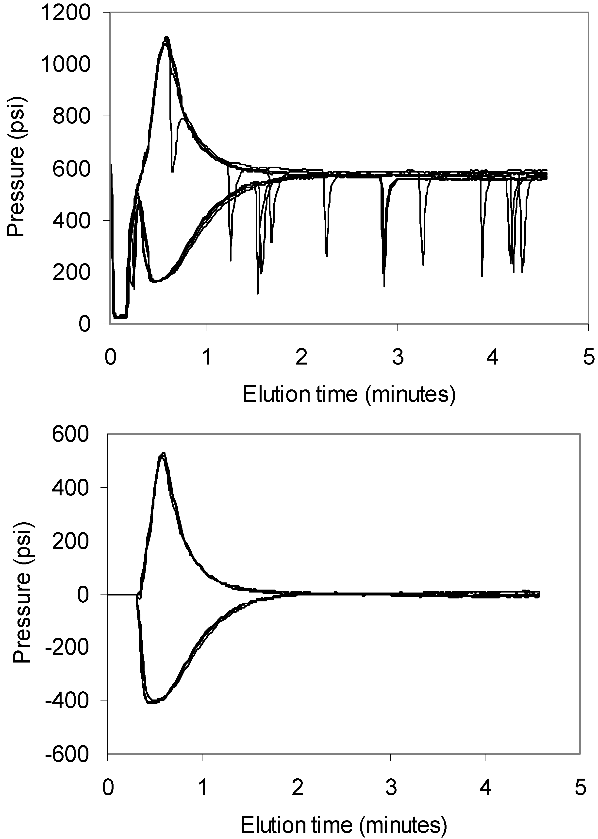
In typical HPLC pumps there are two pistons present, one that is pumping the mobile phase out of its chamber and into the system, and the other one moving in reverse direction while drawing the mobile phase into its chamber. When the pistons exchange their roles, a brief drop of the pressure occurs that is recorded by the transducer. The resulting spikes are seen in
Figure 1. A trivial Microsoft Excel™ macro program was written using embedded Visual Basic that “zapped” the negative spike peaks. The program scanned each profile point by point, and when a sudden drop (>25% of signal magnitude) was encountered, backed up two points to establish starting point for the linear interpolation. The 14th consecutive data point was used as an ending point; thus, the “zapped” region spanned 14 s (one data point was acquired every second). The data shown in
Figure 1 illustrates the effectiveness of the zapping procedure as well as an excellent reproducibility of the method (four, essentially overlapping, runs are shown for each of the two samples). The effect of diffusion is also apparent, as the more viscous samples produced a narrower peak in comparison to less viscous ones. It should be noted that the exact concentration of glycerol in the running phase can vary over the long term due to water evaporation effects. The resulting back-pressure will also depend on the ambient temperature and the temperature in the thermostat, if used. For example, the calibration curves in the following figures intersect the zero line (where peak area is zero) at an apparent glycerol concentration of approximately 75%. Thus, injections of glycerol standards of well-controlled concentrations should be performed during the experiment to assure that the most recent calibration curve is valid.
Figure 1.
Representative profiles of water (lower curves) and 90% glycerol (upper curves). The raw data is shown in upper panel, while the profiles after digital removal of pump pulse spikes are shown in lower panel. Average pressure values between 2 min and 3 min were subtracted from the raw data in upper panel to account for background back pressure in the system. See Materials and Methods section for experimental details.
Generation of a standard curve for the measurement of viscosity using this method was performed using a series of glycerol aqueous solutions of various concentrations. The theoretical viscosity values were first calculated using the approach of Chang [
16], and compared to experimental values published by Dow Chemical Company [
17], and those given in the Handbook of Chemistry and Physics [
18]. However, significant discrepancies were found between the calculated and listed values, e.g., the values for 80% glycerol at 25 °C were 45.9 cP and 47.0 cP at CRC and Dow Chemical tables, respectively, while the calculation method [
16] yielded a value of 80.7 cP. Therefore, the Dow Chemical Company table was employed for the creation of the calibration curve. The values at 25 °C and at glycerol concentrations not listed at the original table were obtained by least-squares fitting to the relation [
19]:
where η is dynamic viscosity, B and D are parameters, E
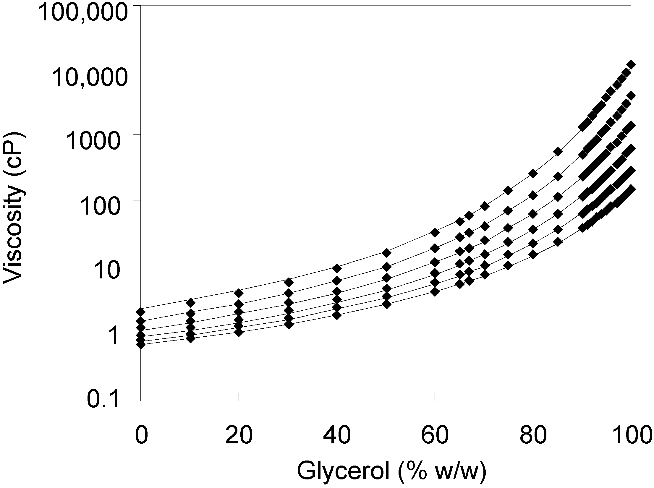
s is the activation energy of viscous flow of solution, R is the gas constant and T is absolute temperature. The data points used for fitting are shown in
Figure 2.
Figure 2.
The viscosities of glycerol solutions at various concentrations listed on the DOW Chemical Company web page at temperatures from 0 °C (top line) to 50 °C (bottom line). The solid lines represent best least-squares fits to Equation (1), using a value of 90 kJ/mol for the energy of activation of viscous flow (Es).
The temperatures from 0 °C (top curve) to 50 °C (bottom curve) at 10 °C intervals were used. A constant value of of 90 kJ/mol the activation energy of viscous flow was found to produce adequate fits, while the values of parameters B and D differed between the concentrations. The values of these parameters at different temperatures, as well as resulting values of dynamic viscosity at 25 °C calculated from Equation (1) are listed in
Table 1.
Table 1.
Parameters for the calculation of viscosity values of glycerol between 0 °C and 50 °C using Equation (1). The value for Ec (activation energy of viscous flow) was 90 kJ/mol. Viscosity values at 25 °C as calculated using Equation (1) are listed for convenience.
Table 1.
Parameters for the calculation of viscosity values of glycerol between 0 °C and 50 °C using Equation (1). The value for Ec (activation energy of viscous flow) was 90 kJ/mol. Viscosity values at 25 °C as calculated using Equation (1) are listed for convenience.
| % (w/w) | B | D | η25 °C (cP) |
|---|
| | | | |
| 0 | 64.526 | 0.096595 | 0.89 * |
| 10 | 64.526 | 0.094838 | 1.06 |
| 20 | 63.716 | 0.093106 | 1.42 |
| 30 | 62.710 | 0.090872 | 1.99 |
| 40 | 61.528 | 0.088231 | 2.95 |
| 50 | 60.012 | 0.084710 | 4.71 |
| 60 | 57.988 | 0.079863 | 8.41 |
| 65 | 56.804 | 0.077022 | 11.8 |
| 67 | 56.256 | 0.075692 | 13.7 |
| 70 | 55.355 | 0.073466 | 17.4 |
| 75 | 53.650 | 0.069230 | 27.0 |
| 80 | 51.654 | 0.064246 | 45.0 |
| 85 | 49.415 | 0.058684 | 80.4 |
| 90 | 46.630 | 0.051654 | 160 |
| 91 | 46.037 | 0.050186 | 187 |
| 92 | 45.333 | 0.048385 | 221 |
| 93 | 44.796 | 0.047127 | 260 |
| 94 | 44.206 | 0.045713 | 308 |
| 95 | 43.503 | 0.043944 | 367 |
| 96 | 42.864 | 0.042414 | 440 |
| 97 | 42.166 | 0.040700 | 531 |
| 98 | 41.435 | 0.038918 | 648 |
| 99 | 40.742 | 0.037274 | 794 |
| 100 | 40.075 | 0.035730 | 976 |
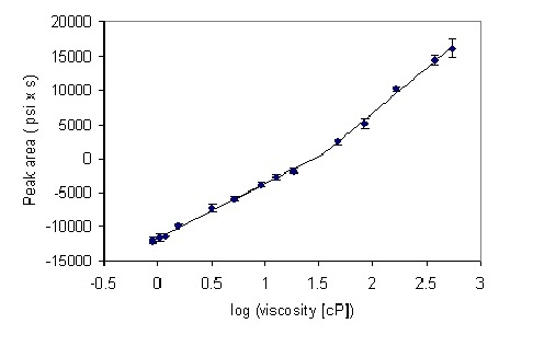
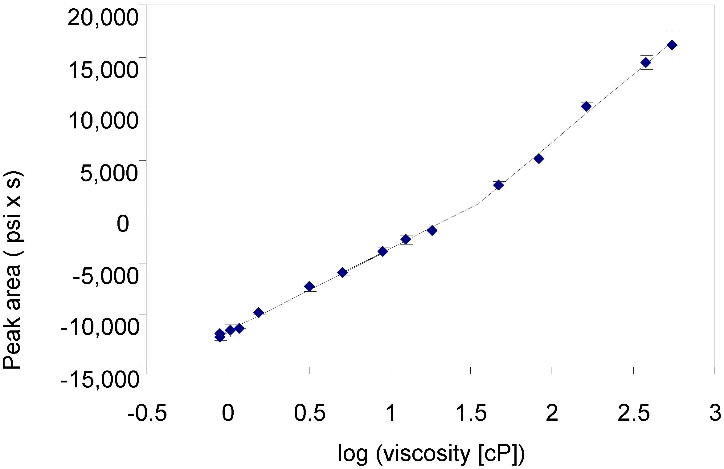
A series of solutions of glycerol were prepared, their viscosities at 25 °C calculated using Equation (1), and their backpressure profiles measured after 10 microliter injections into the HPLC system (see Materials and Methods section for experimental details). At the first approximation, a linear relationship between logarithm of viscosity and the generated pressure was observed (
Figure 3).
However, more detailed inspection reveals a biphasic behavior, where two linear regions of slightly different slopes are discerned. Straight lines were fitted to these regions, leading to the equations for the prediction of viscosity based on the pressure at the pump for the particular system employed. The “cross-over” abscissa (X-axis) point is given by the point of intersection of the two linear fits, calculated from the relation:
where b
1, b
2 and a
1, a
2 are the intersects and slopes of the corresponding straight lines. The X value was 1.54, corresponding to viscosity of 35 cP. The peak area at the “cross-over” point was 702 (psi x second). Thus, for peak areas below 700, an equation y = 7958x − 11541 was used, and for peak area above 700, the equation was y = 13074x − 19412.
Figure 3.
Calibration plot for the series of glycerol standards. Points 1–9 and 10–14 were separately fitted to a straight line by a least-squares procedure embedded in Microsoft Excel™. The error bars show the standard deviation from four measurements.
Figure 3.
Calibration plot for the series of glycerol standards. Points 1–9 and 10–14 were separately fitted to a straight line by a least-squares procedure embedded in Microsoft Excel™. The error bars show the standard deviation from four measurements.
3.3. Measurement of Vaccine and Protein Samples
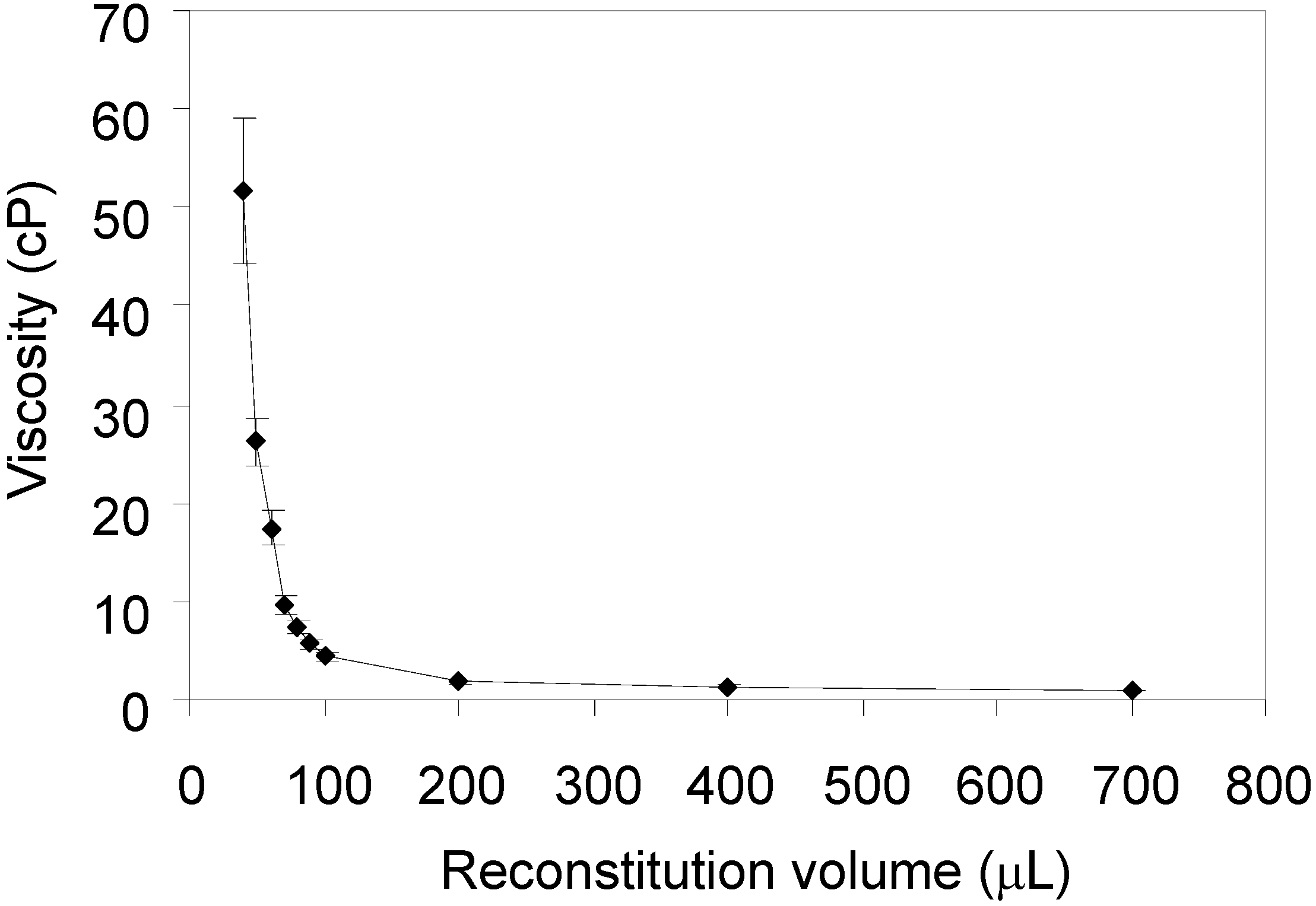
A series of lyophilized Varicella vaccine samples were reconstituted in decreasing volumes of USP water to estimate the highest concentration that maintained reasonable viscosity for injection. Reconstituted samples were placed in HPLC vials and the procedure was executed as described above. The resulting plot is shown in
Figure 4.
Figure 4.
Viscosity values of Varicella vaccine samples, reconstituted in different volumes of USP water, obtained by high-pressure liquid chromatography (HPLC) method. The error bars represent standard deviation of four measurements.
Figure 4.
Viscosity values of Varicella vaccine samples, reconstituted in different volumes of USP water, obtained by high-pressure liquid chromatography (HPLC) method. The error bars represent standard deviation of four measurements.
There was little increase of viscosity between reconstitution volumes of 700 μL and 100 μL. The intermediate range, where the viscosity raised sharply in decreasing reconstitution volumes, fell between 100 μL and 50 μL. At lower reconstitution volumes, the viscosity reached approximately ~50 cP, and the standard deviation also increased, presumably due to the presence of cell debris in the Varicella vaccine preparations, potentially leading to the interactions with surfaces in the sampling system needle and/or tubing surfaces. Furthermore, since the relationship of concentration and viscosity is non-linear, at high concentrations small differences of concentration will result in large changes of viscosity. In general, any differences of concentration between the injections that might be due to sedimentation or surface interactions will tend to increase irreproducibility.
This example illustrates the utility of this method, as a large number of measurements were made using minimal amount of sample. In fact, even smaller amounts would be difficult to handle because of evaporation effects as well as typical lesser accuracy of standard laboratory pipettes at that volume range. The experiment consisted of placing the volumes into the vials, loading the autosampler and starting the pre-programmed method within the HPLC system. After the runs were complete, the set of chromatogram files was exported into an Excel workbook, where the pre-programmed macro performed the removal of the pump pressure spikes, baseline correction, peak integration and the tabulation of the results. Thus, the entire operator’s involvement was in the range of minutes rather than hours, which are often needed for traditional viscometry measurements.
Concentrated solution of bovine serum albumin (~100 mg/mL) was also injected into the system and the pressure was monitored as described above. No signs of increased noise, systems pressure or UV detector artifacts were observed, indicating that the partial dilution into a ~70% glycerol solution did not result in protein precipitation (not shown). The viscosity value, resulting from the procedure describe above, was 82 ± 5 cP. The same sample, when examined with conventional plate viscometer, yielded viscosity of 70 ± 1 cP, suggesting that some variations between the instruments should be expected.
Potential future experiments with a series of concentrated proteins at various viscosities, and examination of the corresponding UV detector profiles may help to evaluate various factors that may contribute to the method’s accuracy and precision. At the present stage, however, the precision of the method allows for use as a tool in the differentiation between various proteins and formulations, in addition to obtaining approximate values of viscosity. In pharmaceutical development practice, the timing of the information and relative ranking are often of high importance, especially because often only a general qualitative range for each critical quality attribute is sought for developability assessment of therapeutic candidates.


