Monetary Transfers in the U.S.: How Efficient Are Tax Rebates?

Abstract

Recent debate on the effectiveness of tax rebates has concentrated on the degree to which they can affect economic activity, which depends on the methodology, the state of the economy, and the underlying assumptions. A better approach to assess the effectiveness of these monetary transfers is by comparing this method to alternative policies—like the traditional monetary injections through the financial intermediaries. A limited participation model calibrated to the U.S. economy is used to show that the higher the proportion of the monetary injection channeled through the consumers—instead of banks—leads to a less vigorous recovery of output but softens the detrimental effect on the utility of the representative household from the inherent inflationary pressure. This result is robust to the relative importance of the injection (utilization of resources) and alternative utility functions.

1. Introduction

As policymakers searched for the optimal way to jump start the recovery from the Great Recession, greater emphasis was placed on alternative policies, like the monetary transfer to consumers recently implemented in the U.S. through tax rebates. Tax rebates were used in the U.S. in 2001 and 2008, with the tax rebates of 2001 injecting approximately $38 billion into the economy (0.2% of GDP), and those of 2008 injecting approximately $100 billion (0.69% of GDP). Although each tax rebate had different stipulations and were implemented under different economic conditions, they were both intended to raise consumption and thus fuel economic growth.

The theory behind these monetary transfers to the consumers is simple: tax rebates increase disposable income and thus should raise consumption levels (according to the marginal propensity to consume), stimulating aggregate demand and consequently creating an economic expansion. Recent findings show that these transfers have been effective in increasing spending (Zandi [1], Broda and Parker [2]), affecting the economy rapidly (Johnson et al. [3], Agarwal et al. [4], Parker et al. [5]), and reaching a broad portion of the economy (Elmendorf and Reifschneider [6], Elmendorf and Furman [7]). Critics, however, argue that, according to the permanent income theory of Milton Friedman or the life cycle theory of Franco Modigliani, consumption only responds marginally because such monetary transfers are only temporary, and thus would not change wealth enough to alter consumption patterns (Eichenbaum [8], Feldstein [9], and Taylor [10,11,12] among others). The Ricardian equivalence reinforces this argument if tax rebates are financed by government debt.

Much of this debate on the effectiveness of tax rebates to generate growth has been centered on its relative success to raise consumer expenditures, measuring the degree of additional consumption generated by this one-time monetary transfer. Recent studies have used survey data from households to examine consumption and saving patterns (i.e., Johnson et al. [3], Agarwal et al. [4], Shapiro and Slemrod [13], Parker et al. [5]), others have used aggregated expenditure data and counterfactual simulations to show what would had happened to consumer spending if no rebate were introduced (Taylor [11,12], Parker et al. [5]), and others have relied on economic modeling to uncover macroeconomic implications (i.e., Elmendorf and Reifschneider [6]). These approaches are dependent on the special characteristics of the economy under which they are being implemented and without a clear and direct comparison with similar but alternative policies. For example, little attention has been paid in comparing these tax rebates, which in essence are cash transfers to a sector of the economy, to the well established monetary injections through the financial intermediaries implemented by the Federal Reserve Bank.

Since these tax rebates are in fact a monetary transfer to the consumer, a more efficient way to assess the effectiveness of these tax rebates should be by comparing them to the traditional monetary injections. By modeling the monetary injection (transfer) in a way in which it targets the financial intermediaries—the traditional way to model monetary injections—or the consumers (effectively putting cash in their hands), we could have a simple and direct way to compare these alternative policies. This approach takes away the dependence on the economic environment (i.e., behavior of savings, the level of indebtness, or high oil prices), as both methods to inject liquidity into the system are subject to the same environment. This approach could also eliminate the discussion of “what would have been our actual expenditures if we didn’t have the tax rebates?”, answer that depends on the circumstances and assumptions used to derive the conclusion, and thus open to interpretation.

Here I evaluate the impact of “governmental” monetary transfers on economic performance, allowing for alternative fractions of a monetary injection to go through financial intermediaries and through the consumers. Using a basic limited participation model (LPM) calibrated to the U.S. economy I show that monetary injections (transfers) have a differential effect on output and on the utility of the representative household depending on the injection distribution between the two alternative channels. The specification with higher percentages of the injection going through consumers produces a weaker and delayed recovery of output, but ameliorates the negative impact of the injection on the welfare of the representative household—transferring money to the household mitigates the drop in consumption arising from the inflationary pressure. This result is found to be robust to alternative degrees of slackness (labor utilization) and use of a utility function with a more predominant role for the intertemporal elasticity of substitution in labor response.

The remainder of this paper is organized as follows: the literature review on the topic is presented in Section 2; Section 3 describes the theoretical limited participation model used to examine this issue; Section 4 presents the main dynamic responses; Section 5 provides some robustness check; Section 6 summarizes and concludes.

2. Literature Review

Tax rebates were included in the Economic Growth and Tax Relief Reconciliation Act of 2001 and in the Economic Stimulus Act of 2008. The rebates are designed to raise consumption and stimulate aggregate demand to generate an economic expansion. These temporary tax rebates differ from permanent changes in tax rates—i.e., a lowering of personal income taxes—since they are temporary and produce lumpy increases in income, which can have important implications for liquidity constrained households (Agarwal et al. [4]). They were first introduced in the U.S. in 2001, when the government transferred $300 or $600 per household (depending on marital status), injecting approximately $38 billion into the economy. Approximately two-thirds of all tax filers received this transfer, with 17% ineligible and 16% not receiving the transfer for non-filing for the rebate (Johnson et al. [3]).

The positive impact that tax rebates can exert on the economy was initially shown by Elmendorf and Reifschneider [6], who used the Federal Reserve Board’s large-scale model to conclude that a one percent of GDP tax rebate would increase output for two consecutive quarters, producing an annualized increase in GDP growth rate of almost four percent [14]. Survey data from this first episode allowed Shapiro and Slemrod [15] to show that around a fifth of the persons who were expecting to receive or actually received the tax rebates were planning on spending the funds. Johnson et al. [3] used microdata to corroborate this finding, showing that households spent between 20% and 40% of the tax rebate during the first quarter, and an additional 30% in the next quarter. The cumulative expenditure was approximately two-thirds of the rebates.

Agarwal et al. [4] used credit card information to provide further evidence of the influence of tax rebates. They found that consumers initially used the tax rebate to reduce credit card debt, but this reduction was reversed in the following quarter to give rise to an increase in consumer spending—with those most likely to be credit constrained producing the largest effect. In addition, Elmendorf and Furman [7] also concluded that the stimulus efforts of 2001 that were focused on individuals (like tax rebates) added a larger effect on spending than skeptical economists might have expected, highlighting that more than 50% of targeted tax rebates were spent within a few quarters. These studies provided evidence of a contemporaneous positive effect on consumption, but also of the presence of a lagged and smaller effect.

The second batch of results come from the 2008 tax rebates, when the government transferred $300 to $600 per individual tax filer, and households could claim an additional $300 per dependent child. On average, individuals received twice as much of what they received in the 2001 tax rebates, enabling them to consume relatively more big-ticket items (Parker et al. [5]). In this instance, the initial prediction indicated that 40% of the tax rebates should have been spent in the following six months (Congressional Budget Office [16]).

Broda and Parker [2] found that recipient households increased their consumption of nondurables by an average of 3.5% in the following four weeks using data collected as tax rebates were mailed out [17]. This represented an expenditure of almost 20% of the tax rebate on the first quarter and an additional 15.5% in the following quarter. With similar data, but in this case from a survey of behavior from the representative household, Shapiro and Slemrod [13] found that only 20% of the households receiving tax rebates planned to spend the rebates, 32% planned on saving the rebate, and almost 50% planned on using the rebate to reduce their debt. This response allowed them to calculate an economy-wide marginal propensity to consume of about one-third. In terms of subsequent consumption, they only found marginal increases in the following quarter.

But Parker et al. [5] actually show that tax rebates have a more significant positive impact on the economy. Using data from the Consumer Expenditure Survey [18] from the third quarter of 2007 to the second quarter of 2009, and estimating a battery of specifications, they find that the tax rebates have created an increase in nondurable expenditures of about 12%–30% of the total stimulus in the first quarter, but the total effect on total consumption can be as large as 50%–90% when one includes all types of consumption (including durable goods). The subsequent quarter also is affected positively, by almost half the contemporaneous effect, but their estimates lack precision. Zandi [1] argues that the one-time tax rebate increased output by more than the initial injection—an estimated total increase in output of 1.26 dollars for each dollar injected. He points out that high oil and food prices precluded the full effect from materializing.

Since targeting becomes crucial for tax rebates to achieve its greatest impact on the economy, the 2008 tax rebates were more targeted to low-income households, who have a higher marginal propensity to consume that produce a larger multiplier effect. Agarwal et al. [4], Johnson et al. [3], Broda and Parker [2], and Parker et al. [5] provide some evidence for these liquidity-constrained households spending a larger proportion of their tax rebate.

However, a problem with the latest tax rebate is that a large proportion of the monetary transfers were saved (Taylor [12], Shapiro and Slemrod [13]), dampening its potential impact on consumption. In fact, Shapiro and Slemrod [13] found that low-income families planned to pay off debt by a higher margin than the rest of the sample, without a clear distinction in their desire to consume. This indicates that low-income households are liquidity constrained in the present but since they will continue to be constrained in the future, they used the tax rebate to reduce debt now and enhance their balance sheet for the future. However, this could be more indicative of a timing issue, since the initial increase in savings (reduction in debt) eventually reverted to an increase in consumption (Agarwal et al. [4]).

Other arguments based on Modigliani’s life cycle hypothesis, Friedman’s permanent income hypothesis, and the Ricardian equivalence further erode the beneficial perception of tax rebates. In fact, many economists used these arguments to criticize the use of tax rebates to raise consumer expenditures (Taylor [10,11], Barro [19]). Taylor [12] relied on empirical evidence to support his view, and used quarterly data on consumer expenditures for the last decade to show that temporary tax transfers have had a very small impact on personal consumption expenditures, but such influence lacked statistical significance.

From a more methodological perspective, and of particular importance to our approach, Parker [20] points out that much of the analysis on the effectiveness of fiscal policy (including tax rebates) during recessions is faulty because the effect of these policies are not measured appropriately. The problem of dynamic stochastic general equilibrium models (DSGE) is the use of linearization around a given steady state (implying that the effect is the same irrespective if one is in a recession or in a boom) and the lack of size specificity of the stimulus (the true effect should be dependent on the size of the stimulus). These limitations are mitigated here by the analysis of alternative channels to inject liquidity, thus controlling for the economic environment, and by the inclusion of a robustness check that controls for the relative importance of the injection, relative to labor income in this case.

3. Theoretical Model

The model used here to study the tax rebate effectiveness is similar to the one used by Vacaflores [21] in his study of cash transfers in Latin America. However, the LPM here introduces a more comprehensive utility function, it is specifically calibrated to the U.S. economy, and is designed to compare the effectiveness of tax rebates relative to the traditional monetary injection—providing an extensive robustness check to verify the stability of the results. Theoretical models are ideal to conduct counterfactual policy experiments, as they can be calibrated to approximate a given economy and thus examine the dynamics emanating from the implementation of alternative policies. Of course, they are calibrated to a given state of the economy (normal conditions), and thus fail to incorporate unusual behavior, like the failure of the financial intermediaries to lend at normal levels, the reluctance of firms to invest even when they had the funds, and the unwillingness of households to consume at normal levels.

This LPM requires that the representative household determines their money allocation between cash to finance consumption ( ) and deposits to earn a return ( ) one period in advance, such that when agents want to alter their money holdings they will face an adjustment cost—the subscript t means the corresponding variable at time t. This implies that bank deposits would not change significantly following a monetary shock, generating a large and persistent liquidity effect. A monetary injection then increases the amount of funds available for lending, and the firm could take advantage of the lower interest rate.

3.1. Structure of the Model

The economy is characterized by perfect competition, with the production of an identical good being performed by domestic firms and also by firms from the rest of the world. The law of one price holds and the price of the identical good is given by P_t (dollars). Letting s_t denote the price of foreign currency in terms of domestic currency (i.e., euros per dollars), and keeping in mind that the small open economy assumption implies that the price of the good in foreign currency P^* is exogenous, then purchasing power parity is given by:

P_t = s_tP^*

(1)

3.1.1. The Household

The representative agent’s objective is to choose a path for consumption and asset holdings to maximize:

(2)

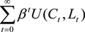where C is real consumption and L is leisure hours. We normalize the time endowment to unity, so leisure is given by L_t = 1 − H_t − Ω_t, where H is labor supply and Ω is time spent adjusting money balances (this reduces leisure time and thus become a time cost). The adjustment cost is given by:

(3)

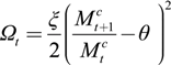with the parameter ξ calibrating the size and persistence of the liquidity effect, and θ being the steady state money growth rate.

We use a utility function that defines consumption and leisure as complements, as proposed by Greenwood, Hercowitz, and Huffman [22]. This specification has important characteristics useful for the analysis of economies with different degrees of idle resources. The per-period utility function is given by:

(4)

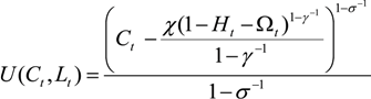where γ is the Frisch-elasticity of labor supply (0 ˂ γ) , and σ is the inverse of the intertemporal elasticity of substitution in the usual Constant Elasticity of Substitution (CES) utility function. The parameter χ calibrates the weight of leisure in the utility and is endogenously determined—see steady state derivation.

The cash-in-advance (CIA) constraint has the usual allocation on money cash ( ) brought forward from period t−1, but we also allow for the government to transfer money that can be used for current consumption:

(5)

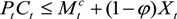X_t is the amount of money transferred to the consumer and the parameter φ is the proportion of the monetary transfer (injection) channeled through the financial intermediary. A monetary transfer (injection) could be fully channeled through the financial intermediaries when φ is equal to one (the usual monetary injection) but could also be channeled towards the consumers—and thus consumption —when φ is set below one [23].

Households have access to domestic and foreign financial markets. The household budget constraint is then given by:

(6)

At time t the household determines consumption C_t and labor supply H_t, as well as the amount of money deposited in banks, , the amount of money kept as cash, , and the foreign asset position B_t+1. Household income is determined by the real wage w_t and the profits (or dividends) received at the end of the period from the firm and the commercial bank, and , as well as interest on deposits and on foreign bonds. Foreign bonds yield a risk-free nominal interest rate .

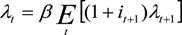
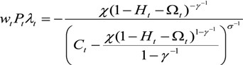
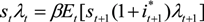
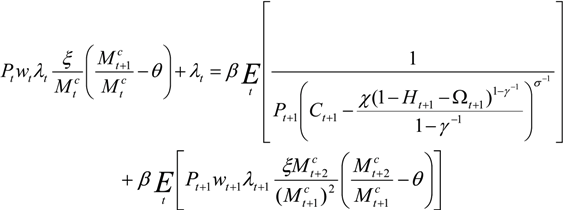
The household’s maximization problem can be represented by the value function: , subject to the cash-in-advance constraint (Equation (5)) and the budget constraint (Equation (6)). Here refers to the expected value of the term(s) in brackets conditional on information up to time t. Letting λ_t denote the Lagrangian multiplier associated with the budget constraint, the first order conditions for the household’s choice of consumption, labor, money deposits, money-cash holdings, and foreign assets provide the following relationships:

(7)

(8)

(9)

(10)

Equation (7) reflects equality between the costs and benefits of bank deposits, while Equation (8) entails equality between the marginal disutility of working and the marginal benefit—the real wage multiplied by the Lagrange multiplier. Equation (9) indicates equality of the current marginal cost of buying foreign assets (in terms of wealth) with the gains in the following period from holding such assets today, and Equation (10) equates the costs and benefits related to the choice made at time t of money holdings available for consumption in the following period. It is clear that if the adjustment cost is zero (ξ = 0) then Equation (10) will just equate the household’s cost of holding money in the current period to the marginal utility of consumption in the following period, properly discounted.

3.1.2. The Firm

We use the typical Cobb Douglas production function to represent the firm’s production technology:

(11)

where α ∈ [0,1], z is the technological shock and K is physical capital. The firm maximizes the discounted stream of dividend payments, considering the value of this discounted dividend stream to the owners, the households.

We assume that firms can only borrow for incremental investments, which need to be paid off completely by the end of the period, with the cost of borrowing given by the nominal interest rate i_t. Consequently, the nominal profits of the firm are given by:

(12)

with investment evolving according to the law of motion of the stock of physical capital,

(13)

where δ is the depreciation rate. The last term in Equation (12) accounts for the fact that physical capital is not freely adjusted but in fact forces firms to incur a capital adjustment cost when altered. Here the parameter ψ is chosen to calibrate such cost.

The decision about the use of dividends, either payments to households or reinvestment in the firm, is captured by the ratio of the multipliers associated with the budget constraint of the household in the value function (see Equation (7)), as it reflects the consumer’s variation in wealth (which is time varying). The value function of the firm is then

(14)

The first order necessary conditions for the household’s choice of labor and capital produce the standard results. The fact that the cost of hiring an additional worker should equal the worker’s marginal productivity is reflected in Equation (15), and the requirement that the cost and benefits of marginal investment should be the same is reflected in Equation (16).

(15)

(16)

3.1.3. The Monetary Authority

Tax rebates are part of fiscal policy, and thus are administered by a different entity than the one that conducts monetary policy (the Federal Reserve Bank). Here we abstract from this technicality and assume that these monetary transfers could potentially be administered by the same authority that conducts the monetary injections [24]. We are therefore postulating that the “government” injects money into the system, through the financial intermediary or through the consumers, leaving the practical implementation considerations aside. That is, the “government” controls the money supply according to:

M_t+1 = M_t + X_t

(17)

where the monetary authority’s injection is defined as X_t = (θ_t – 1)M_t, and where θ_t represents the monetary growth factor.

3.1.4. The Financial Intermediary

At the beginning of the period, financial intermediaries receive deposits from the household and potentially a monetary injection from the monetary authority, φX_t [25]. Its nominal asset balance is given by:

(18)

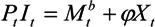where P_tI_t are the loans made to firms (investment) and the right hand side are the source of funds.

The per-period profits of these financial intermediaries are equal to the interest on loans minus interest paid on deposits in the bank. Here we assume that the lending rate and the deposit rate are the same, so the bank earns zero economic profits unless there is a monetary injection. The monetary injection directly into these banks then is a subsidy to the bank since there is no interest expense incurred by the bank on the use of such funds.

(19)

3.2. Closing the Model

The household’s budget constraint (Equation (6)) under market equilibrium provides the path for the holding of foreign assets:

(20)

The right-hand side of the equation relates the foreign assets position to the difference between domestic production and absorption in the economy, giving the balance of payments equilibrium.

To avoid the typical non-stationarity issues from incomplete asset markets, we also introduce the interest rate differential on bond holdings as in Karamé et al. [26]:

(21)

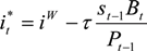
The interest in bonds is determined by the world interest rate and the net real foreign asset position, with τ calibrating the asset position. This assumption leads to a lower bond interest rate as the country’s net asset position improves.

The dynamics of this model are generated by a monetary shock and a technology shock. Both shocks are modeled in the usual form, with the monetary shock given by:

(22)

where ε_θ,t+1 is white noise innovations with variance , and the technology shock denoted by:

(23)

with ε_z,t+1 being the white noise innovation with variance . ρ_θ and ρ_z are the respective persistence parameters, while θ and z are the steady states of θ and z, respectively.

The set of equations given by the first order conditions, the market equilibriums, and the laws of motion for physical capital, domestic money supply, foreign assets, and the monetary growth factor constitute a non-linear dynamic stochastic system, and are presented in the Appendix (A) in Vacaflores [27].

3.3. Calibration and Steady State Equilibrium

The calibration of the model to the U.S. is presented in Table 1 below. It uses standard values for the capital share, α, the subjective discount factor, β, and the depreciation rate of capital, δ. We set the parameter H to 0.2, which implies a 34-h work week. The long-run gross inflation factor is given by π, and is determined by the average money growth rate θ from the measure of M1 (0.8% per quarter), obtained from the Federal Reserve Bank of St Louis’s FRED data base. The data is seasonally adjusted and at quarterly frequency, it starts in the first quarter of 1990 and ends on the third quarter of 2008—after this date our measures of monetary policy are no longer appropriate indicators due to the policies of the Federal Reserve Bank to contain the financial crisis.

Table 1. Model calibration values.

α = 0.36	ν = −0.0288	ξ = 3	σ = 1.05	H = 0.2
β = −0.988	θ = 1.0083	φ = 0.1	τ = 0.0019	δ = 0.025
ρθ = 0.29	σθ = 0.00194	γ = 1.05	ρz = 0.95	σz = 0.00816

Table 1. Model calibration values.

α = 0.36	ν = −0.0288	ξ = 3	σ = 1.05	H = 0.2
β = −0.988	θ = 1.0083	φ = 0.1	τ = 0.0019	δ = 0.025
ρθ = 0.29	σθ = 0.00194	γ = 1.05	ρz = 0.95	σz = 0.00816

I have also used FRED’s measures of real GDP, real consumption, real investment, interest rate, exchange rates, and trade balance to judge the model’s adequacy. This information allows us to calibrate the economy to reflect an average trade deficit as percentage of GDP of 2.877%—which in the steady state calculations will be represented with the parameter ν to simplify equation 20.

The choice on the responsiveness of the interest on foreign bonds to the actual level of bonds (τ) follows Karamé et al. [26], and the parameter σ is set to be greater than 1 to reflect complementarity between leisure and consumption is the CES case (robustness section). The Frisch-elasticity of labor supply (γ) is set to 1.05, very close to the value chosen by Nakamura et al. [28]. While the parameters describing the technological shock are standard, we take a bit ad hoc approach with the calibration of the persistence coefficient of the monetary shock, ρ_θ. We usually take the persistence of the money supply to anchor the behavior of money, but here we opt for calibrating it to be between the actual persistence of the 2008 tax rebates (0.19) [29] and the persistence parameter from the estimation of the AR(1) process on M1 (0.56)—we use the estimated standard deviation, σ_θ, to describe the monetary innovation.

We consider the case of a small but positive adjustment cost parameter, ξ = 3, which represent lost time rearranging money balances of less than a minute per week. Nominal variables are made stationary by dividing them by the lagged domestic price level. The main variables are: ; ; ; ; . Obviously adjustment costs disappear in the steady state, and values do not need time subscripts. We look at a steady state in which the domestic and foreign inflation levels are the same, so purchasing power parity implies that the change in the nominal exchange rate is constant [30]. Consequently, the uncovered interest rate parity condition implies that the domestic interest rate and the interest rate on foreign bonds are equal (i = i^*). The calculation of steady state equilibrium is straight forward, and a detailed explanation of its derivation is available in Vacaflores [27] under the section Appendix (B).

The steady state values presented below in Table 2 examine the allocation of resources in the small open economy, representative of the U.S. economy. Note that we are not modeling an economy with a government, so we omit taxes and government spending and thus concentrate on consumption, investment, and net exports.

Table 2. Steady state values.

	100% Injections towards Investment	Percent of Output
Nominal Interest Rate	0.0202	-
Interest on Foreign Bonds	0.0202	-
Investment	0.1685	0.23
Physical Capital	6.7402	-
Output	0.7095	1.00
Hours Worked	0.2	-
Real Wages	2.2705	-
Consumption	0.5615	0.79
Real Money Balances	0.7300	-
Real Money Cash	0.5660	-
Real Money Deposits	0.1640	-
Inflation	1.0080	-
Foreign Bonds	1.6825	-
Trade Balance	−0.0204	−0.028

Table 2. Steady state values.

	100% Injections towards Investment	Percent of Output
Nominal Interest Rate	0.0202	-
Interest on Foreign Bonds	0.0202	-
Investment	0.1685	0.23
Physical Capital	6.7402	-
Output	0.7095	1.00
Hours Worked	0.2	-
Real Wages	2.2705	-
Consumption	0.5615	0.79
Real Money Balances	0.7300	-
Real Money Cash	0.5660	-
Real Money Deposits	0.1640	-
Inflation	1.0080	-
Foreign Bonds	1.6825	-
Trade Balance	−0.0204	−0.028

As it can be observed, our small open economy has an inflation rate of 0.8% per quarter, which leads to a nominal interest rate of 2.02% per quarter. Investment in this small open economy without government is almost 23% of GDP while consumption is approximately 79% of GDP, with the trade deficit allowing for these higher levels (around two percent of GDP).

4. Dynamic Response

We first evaluate the ability of our LPM to generate standard results from monetary (and technological) shocks [31]. In particular, we analyze the aggregate dynamics of inflation, the nominal interest rate, the nominal exchange rate, consumption, labor supply, and output, examining such dynamics under a baseline calibration where the complete monetary transfer goes through the financial intermediaries. Since we are considering a small open economy, exogenous foreign variables are held constant and drop from the dynamics.

The impulse response functions presented in this section are those following a one percent increase in the domestic money growth rate in the initial period. As shown below in the top-left panel of Figure 1, the monetary shock puts an upward pressure on inflation, creating a one period price increase of almost two percent. This higher inflation reduces the value of real money balances, inducing households to reallocate more funds towards cash in order to preserve future consumption. However, since households cannot withdraw their deposits immediately, and since the monetary expansion goes through the financial intermediaries, these excess of funds available for lending outweigh the inflationary pressure and produce a drop in the nominal interest rate, by approximately 10 base points. This is the typical liquidity effect, and its persistent impact on the interest rate can be observed below in the top-center panel of Figure 1.

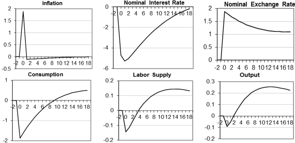
Figure 1. Dynamic response to a 1% monetary shock. Percent deviation from steady state in vertical axis and quarters in horizontal axis.

Figure 1. Dynamic response to a 1% monetary shock. Percent deviation from steady state in vertical axis and quarters in horizontal axis.

The spike in inflation has a direct and immediate effect on the exchange rate, leading to an instantaneous depreciation of the nominal exchange rate of similar magnitude than the rise in prices. The overshooting of the nominal exchange rate shown in the top-right panel of Figure 1 is due to the uncovered interest rate parity, which requires the interest rate differential to be equal to the expected rate of appreciation of the following periods, leading to the subsequent appreciation until it stabilizes at its higher steady state, as the liquidity effect dissipates. The fall in the nominal interest rate also reduces the return on domestic savings, and forces the household to reallocate more funds towards foreign assets.

The higher inflation and the inability to reallocate funds contemporaneously have a direct impact on consumption, as shown in the bottom-left panel of Figure 1. In this model, since consumption is determined by the cash-in-advance constraint, and since the amount of money-cash available for consumption is predetermined, inflation generated by the larger money supply reduces consumption instantaneously [32,33]. The consumption dynamics from the second period onwards arises from the rearrangement between money-cash and money-deposits, which is done slowly to avoid a one-time large adjustment cost. Consumption recovers smoothly, reaching the original steady state level of consumption by the ninth quarter and remaining at above steady state levels for an extended period of time.

The dynamics governing production are presented in the last two panels in the bottom of Figure 1. It is well known that expansionary monetary shocks generate a positive wealth effect that allows for an increase in leisure (a drop in labor supply), but since capital is fixed for the period, this lower supply of labor leads to a slight drop in output on impact. However, this instant drop is quickly reversed as capital accumulates—investment increases as a response to the below steady-state interest rate—and labor supply recovers to levels above the initial supply—from the above-steady-levels of real wages. Output returns to its original steady state level two quarters after the monetary shock and peeks after 12 quarters before starting to decline again—the typical hump-shape response (i.e., Christiano and Eichenbaum [34]).

To assess the model accuracy, we now report the volatility of the main macroeconomic aggregates and their correlation with respect to output. The upper portion of Table 3 shows the unconditional moments for the actual data for the period 1990 quarter 1 through 2008 quarter 3, expressed in growth rates. One can see that investment is more than 5 times more volatile than output while the nominal interest rate is approximately 25 times more volatile than output. Consumption and inflation are slightly less volatile than output, and the nominal exchange rate is over 4 times more volatile than output. If we consider the correlation of our aggregates with respect to output, we find that there is a positive correlation between the investment, interest rate, and consumption with output, with the correlation of investment and output being the largest and the correlation between the interest and output being the smallest. We also observe a negative correlation of inflation and the exchange rate with output, with the correlation of inflation with output being slightly larger than the correlation of the exchange rate and output.

In terms of the model simulations, the model provides volatilities that are comparable to those coming from the data—except those for inflation and nominal exchange rate [35]. In particular, the relative volatilities of investment, the nominal interest rate, and the nominal exchange rates are still large (although approximately half as large as in the data). In terms of output correlations, the aggregates have the same tendency as the data and their magnitudes are closely comparable. Although the simulation generates correlations of investment, the interest rate, and consumption with output that are slightly larger, their relative correlation with output remains intact. The correlation of inflation and output in the simulation is similar to the data, but the correlation of the exchange rate and output is almost four times larger than the data. The data and the model present similar moments.

Table 3. Unconditional moments.

Data	Standard Deviation	Relative Standard Deviation	Correlation with Output
Output	0.5392	1.00	1.0000
Investment	2.9170	5.40	0.7385
N. Interest Rate	13.5008	25.03	0.2991
Consumption	0.4805	0.89	0.6262
Inflation (CPI)	0.4741	0.88	−0.2247
N. Exchange Rate	2.2070	4.09	−0.1567
Model
Output	0.0272	1.00	1.00
Investment	0.0619	2.27	0.95
N. Interest Rate	0.3093	11.37	0.70
Consumption	0.0483	1.77	0.85
Inflation	0.0322	1.18	−0.17
N. Exchange Rate	0.0491	1.80	−0.53

Note: Variables were transformed to growth rates (∆lnX) in the data estimation, using FRED’s data. Model estimates are obtained using H-P simulations. Data starts in 1990Q1 and ends in 2008Q3.

Table 3. Unconditional moments.

Data	Standard Deviation	Relative Standard Deviation	Correlation with Output
Output	0.5392	1.00	1.0000
Investment	2.9170	5.40	0.7385
N. Interest Rate	13.5008	25.03	0.2991
Consumption	0.4805	0.89	0.6262
Inflation (CPI)	0.4741	0.88	−0.2247
N. Exchange Rate	2.2070	4.09	−0.1567
Model
Output	0.0272	1.00	1.00
Investment	0.0619	2.27	0.95
N. Interest Rate	0.3093	11.37	0.70
Consumption	0.0483	1.77	0.85
Inflation	0.0322	1.18	−0.17
N. Exchange Rate	0.0491	1.80	−0.53

Note: Variables were transformed to growth rates (∆lnX) in the data estimation, using FRED’s data. Model estimates are obtained using H-P simulations. Data starts in 1990Q1 and ends in 2008Q3.

4.1. Alternative Distributions of Monetary Injections

To determine if there is a differential effect from monetary injections (transfers) on the economy we now allow for alternative distributions of the monetary injection between financial intermediaries and consumers. To this end, we allow the parameter φ to vary from 1, thus reducing the percentage of monetary injection going through the financial intermediary and increasing the percentage going through the consumers. We consider the cases of φ equal to 1, 0.8, 0.6, and 0.4, for the proportion of the injection being channeled through the financial intermediary—and not through consumers [36].

Figure 2 below presents the dynamic response of the interest rate, investment, capital, consumption, labor supply, and output. The monetary injection has no differential effect on inflation, and the nominal exchange rate, when the proportion channeled through the consumer increases. However, when one reduces the percentage of the monetary injection going through the financial intermediary the drop in the nominal interest rate is slightly reduced since the amount of funds available to the financial intermediary are relatively smaller. The initial drop in the interest rate is almost 20% (40%) smaller as we reduce the amount of money injected through the financial intermediary from 100% to 80% (60%). However, the additional interest drop in the period following the shock is enhanced as the proportion of the money injected through the financial intermediary is decreased—the fall in real money deposits is smaller for larger proportions of the monetary injection going through the consumer. This smaller liquidity effect has implications for the investment amount, and capital accumulation, as observed in the next two panels in the top of Figure 2. In fact, the original increase in investment declines as the proportion on the monetary injection going through the financial intermediaries is reduced, being slightly overturned for the case when only 40% is channeled through the financial intermediaries.

As shown in the bottom-left of Figure 2, despite the fact that the inflationary effect is identical under the different distributions of the monetary injection, thus suggesting a similar drop in consumption due to the predetermined allocation of money cash, the proportional increase of the monetary injection towards consumption leads to a smaller initial fall in consumption. Higher fractions of the injection going through consumers loosen the cash-in-advance constraint and thus partially neutralize the inflationary pressure, or loss of purchasing power of real money cash. The subsequent dynamics are almost unaffected by the alternative distribution of the injection between the financial intermediaries and the consumers.

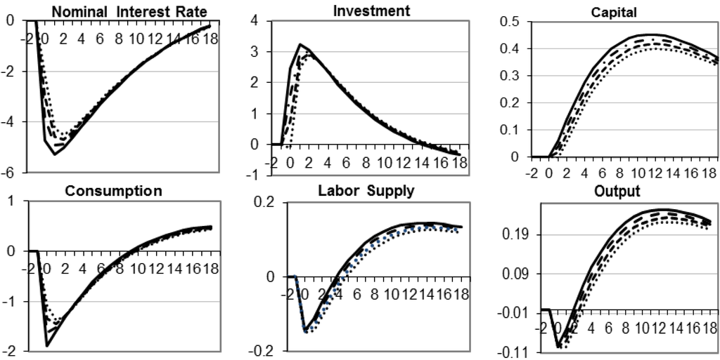
Figure 2. Dynamic response to a 1% monetary shock. Percent deviations from steady state in vertical axis and quarters in horizontal axis. φ = 1, ^____; φ = 0.8, ---; φ = 0.6, ∙ ∙ ∙; φ = 0.4, ∙∙∙.

Figure 2. Dynamic response to a 1% monetary shock. Percent deviations from steady state in vertical axis and quarters in horizontal axis. φ = 1, ^____; φ = 0.8, ---; φ = 0.6, ∙ ∙ ∙; φ = 0.4, ∙∙∙.

We also observe that on impact the response of labor is unaffected by the alternative distributions of the monetary injection, but we find that the recovery in labor supply is diminished, and even delayed, by the increasing channeling of larger proportions of the monetary injection through the consumers. Labor initially falls in response to the positive wealth effect, but then responds to the behavior of real wages, which mimics the behavior of capital and presents a smaller—and even small reduction—subsequent improvement in real wages as we reduce the proportion of the monetary injection going through the financial intermediary. Of course, since the initial drop in labor is unaffected and the amount of capital predetermined, the initial drop in output is unaffected by the alternative distribution of the monetary injection. However, since the recovery of labor and accumulation of capital is diminished by the larger proportions of the monetary injection channeled through consumers, the subsequent recovery of output is also reduced when we direct a higher fraction of the injection towards the consumer. Actually, the peak is 13% smaller than the base line case when 60% of the injection is being channeled through the consumers, and the gap remains significant for a prolonged period of time. While the per-period differences might not be large, the cumulative effect has a long lasting impact on economic recovery.

While it should be clear that the most efficient way in which the government could inject liquidity into the system is by the traditional monetary injections, and not through the alternative tax rebates, the fact that people’s wellbeing (utility) plays an important role in policy decision making, it becomes imperative to also examine the utility response to these alternative distributions of the injection. In Figure 3 below we present the behavior of the per-period utility of the representative household under the four alternative distributions of the injection between the financial intermediaries and consumers.

Figure 3. Utility dynamics. Percent deviations from steady state in vertical axis and quarters in horizontal axis.

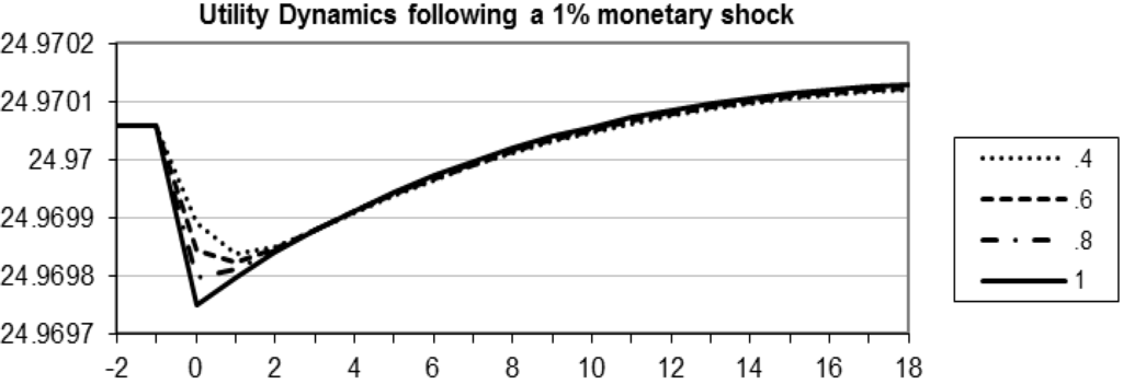
Figure 3. Utility dynamics. Percent deviations from steady state in vertical axis and quarters in horizontal axis.

Figure 3 shows that the expansionary monetary shock reduces the utility of the representative household on impact irrespective of the way in which the government injects liquidity into the system. The drop in consumption and the time lost rearranging money balances to preserve future consumption is larger than the benefit from the initial increase in leisure from the wealth effect. However, it also shows that the magnitude of the initial decline in utility is dependent on the distribution of the monetary injection between the financial intermediaries and consumers. As we increase the proportion of the injection being channeled through consumers, the initial drop in consumption weakens, reducing the downward pressure in utility, and this small deviation in consumption also reduces the amount of time spent by the representative household adjusting money balances, again reducing the initial drop in utility (A more comprehensive analysis will account for all future periods, but since all responses converge to the same level after four periods this conclusion still holds).

While not directly comparable because of more persistent dynamics, the initial drop in utility from the 1% positive monetary injection is equivalent to a 0.6745% (0.576%) negative technological shock when 100% (80%) of the injection goes through the financial intermediary. In terms of utility, channeling higher proportions of the monetary injection through consumers is equivalent to reducing the magnitude of a technological shock.

Tax rebates in a sense help protect household’s consumption patterns, and by mitigating these drops in consumption these transfers generate the intended economic expansion. That tax rebates protect consumption patterns should not be surprising, but a specific measure of its contribution to consumer expenditures could facilitate a better measurement of the overall contribution to utility. The effectiveness of tax rebates, relative to the typical monetary injection, depends on the objective that one is trying to achieve: if one wants to get economic recovery in the most efficient way, then greater proportions of the injection should be channeled through the financial intermediaries. But if one is trying to maximize the wellbeing of the populations, the results indicate that larger proportions of the injection should in fact be channeled through consumers—to the extent that consumers will only use these funds towards consumption according to the MPC, then some fraction will still be going through the financial system to still produce the interest rate reduction.

5. Robustness of the Differential Effect

In order to establish the robustness of our results, we examine the dynamic response of the main macroeconomic aggregates from alternative levels of labor participation and from a more flexible utility function. The examination of alternative degrees of labor participation arises from the extensive arguments indicating that the effectiveness of a given policy depends in the amount of resources that could be mobilized. Here we model the existence of larger labor participation by increasing the intensive margin of labor (by increasing the level of H). Increasing the steady state level of labor supply will be equivalent to having an economy with a higher number of worked hours (per employee), such that the overall response of consumers to the monetary transfer should be smaller. In Figure 4 below we examine the case when households supply 25% of its total time to labor activities (approximately 42 h per week) in the center column, and the case when they supply 30% of its total time to labor activities (approximately 50 h per week).

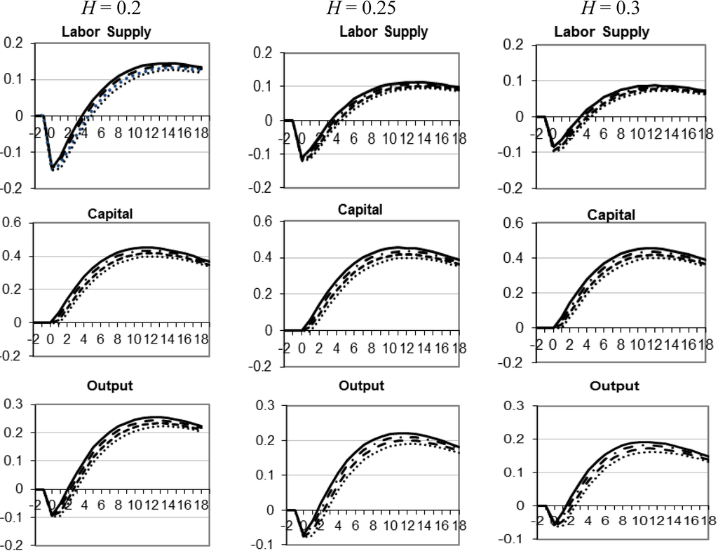
Figure 4. Dynamic response to a 1% Monetary shock under alternative hours worked. Percent deviations from steady state in vertical axis and quarters in horizontal axis. φ = 1, ^____; φ = 0.8, ---; φ = 0.6, ∙ ∙ ∙; φ = 0.4, ∙∙∙.

Figure 4. Dynamic response to a 1% Monetary shock under alternative hours worked. Percent deviations from steady state in vertical axis and quarters in horizontal axis. φ = 1, ^____; φ = 0.8, ---; φ = 0.6, ∙ ∙ ∙; φ = 0.4, ∙∙∙.

Relative to the base line calibration (left column), the increase in labor participation reduces the importance of the wealth effect from the monetary injection, and thus creates a smaller initial drop in labor supply, and a subsequent smaller recovery as the monetary shock dissipates. In the three cases presented, the reduction of the proportion of the injection being channeled through the financial intermediaries continues to diminish the subsequent recovery of labor by similar proportions. However, the effect of the positive monetary shock on the interest rate, and thus on investment and capital accumulation, is unaffected by the degree of labor participation, so the dynamics of capital to alternative distributions of the injection between financial intermediaries and consumers is the same for the different levels of labor participation (moving rightwards through the columns). This leads to an output response that preserves the differential impact of alternative distributions of the injection between financial intermediaries and consumers but that present a more subtle response to the monetary shock as the degree of labor participation is enhanced—since the response of capital is identical, the labor dynamics drive this response.

These results corroborate the intuition that the existence of idle resources—lower utilization of labor—would lead to a more pronounced effect from policies. Here this result arises from the fact that higher levels of labor participation increases labor income, such that the same size monetary shock is relatively less influential and thus creates a relatively smaller wealth effect, with its consequent influence on labor supply. This effect can also help explain the arguments that emphasize on the size of the injection (stimulus) to achieve a given recovery. Discussions of the 2008–2009 policy response had some economists pushing for a higher stimulus (i.e., Krugman [37]) while others were reluctant to any stimulus (i.e., Taylor [10,11,12]). More than the overall size of the stimulus, we are able to capture the relative importance of the stimulus relative to labor income of the recipients. This also suggests that, in order to achieve the most “bang for the back” from monetary transfers, policymakers should target the transfers to low-income households, most credit constrained individuals or families. The recent temporary tax rebates partly achieved this by providing a differential return according to the reported income tax level, but it was not as efficient as it could be because a large portion of the U.S. population does not pay taxes, and consequently did not participate of the tax rebate [38].

The second sensitivity verification arises from the need to test the robustness of the responses to alternative specifications of preferences, giving that we have an array of alternative utility functions that could potentially reflect household behavior better. In addition, since the output response to the monetary shock depends on the labor response to the wealth effect, we would like to introduce a utility function that has the intertemporal elasticity of substitution (IES) playing a more predominant role. The constant elasticity of substitution (CES) utility function fulfills these requirements, so we use it to describe preferences:

(24)

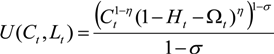where η is the relative weight of leisure (0 ˂ η ˂ 1) and σ is the inverse of the IES (here assumed to be equal to 1.05 to retain the complementarity property between consumption and leisure used in the main utility function) [39].

As it can observed in Figure 5, the monetary injection produces similar responses to the standard ones found with our original utility specification. Inflation and the exchange rate are barely affected by the alternative distribution of the monetary injection. However, the use of this CES utility function brings to light a differential response of labor supply to the monetary shock, and to the alternative distributions of the injection between the financial intermediaries and the consumers. Here we find that while the monetary shock reduces labor supply on impact at similar rates than the original specification, the subsequent behavior of labor is affected by the CES specification. Also, the relatively smaller drop in the interest rate provides a smaller boost in investment—and accumulation of capital—that when combined with the initial contraction in labor generates a higher real wage that provides the incentive for labor to increase its supply (just like in the original case). The recovery of labor here is smaller, and returns only slowly to the original steady state, with the higher proportion of the injection towards the consumer in this case producing a relatively greater recovery in the supply of labor.

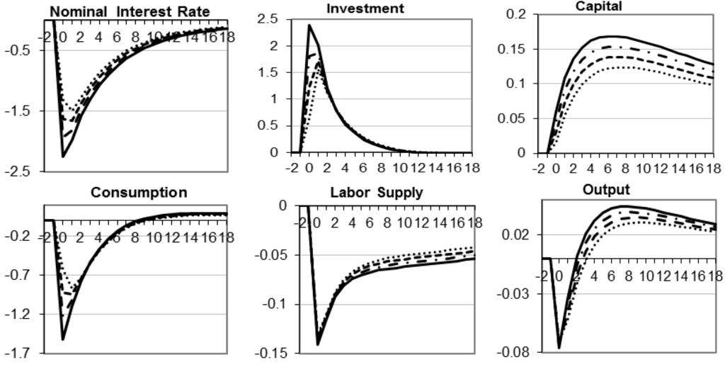
Figure 5. Dynamic response to a 1% monetary shock under CES utility function. Percent deviations from steady state in vertical axis and quarters in horizontal axis. φ = 1, ^____; φ = 0.8, ---; φ = 0.6, ∙ ∙ ∙; φ = 0.4, ∙∙∙.

Figure 5. Dynamic response to a 1% monetary shock under CES utility function. Percent deviations from steady state in vertical axis and quarters in horizontal axis. φ = 1, ^____; φ = 0.8, ---; φ = 0.6, ∙ ∙ ∙; φ = 0.4, ∙∙∙.

Since the behavior of investment and capital are similar—although smaller from the relatively large IES—than in the baseline case, the behavior of labor to these alternative distributions of the injection is what drives the output response. The relative smaller stock of capital coupled with a minute recovery of labor produce the typical hump-shape response that in this case peaks at a lower level, but the qualitative finding that such recovery is diminished by the larger distribution of the injection towards consumers remains clear. Irrespective of the utility function, output initially drops but quickly recovers and stays above steady states for a significant period (see also Vacaflores [21] for the results for logarithmic preferences).

6. Conclusions

The effectiveness of tax rebates to households to fuel economic expansions remains questionable. Problems in the assessment of its effectiveness arise from the type of data (micro data vs. macroeconomic aggregates), the type of methods employed (techniques that do not control for the asymmetrical response of policies to alternative environments), and from the specific assumption with regards to the expected response of the receivers—in terms of consumption. We avoid these inherent complications by examining the effectiveness of tax rebates in terms of its efficiency relative to conventional monetary policy.

The dynamic responses of the macroeconomic aggregates in this study are similar to a substantial literature in monetary policy, especially in terms of the liquidity effect of the interest rate and hump-shape response of output. The dynamics clearly indicate that the most effective way in which the government could inject money into the economy to create economic recoveries is in fact by channeling such injections through the financial intermediaries. However, since the expansionary monetary shock reduces the utility of the representative household, an increase in the percentage of the monetary injection being channeled through the consumers will also mitigate the negative impact on the utility. These results are robust to the degree of utilization of economic resources – suggesting that its effectiveness depends on the degree of idle resources—and to alternative utility functions.

While technically these monetary transfers are conducted by separate entities, it is not farfetched the idea that the Fed could operationally implement monetary transfers to the consumers—remember that Bernanke [40] practically laid out the possibility for the Fed to drop money into the consumers (with the cooperation of the government). We abstract from this technicality and provide a model that enables the “government” to inject money into the system through the financial intermediaries or through the consumers. This model thus allows policymakers to measure the relative effectiveness of these alternative policies.

Further research should be conducted on the degree of responsiveness of consumption to these temporary tax rebates, and the determination of optimal expansionary policy should consider the targeting and timing of such monetary transfers. In fact, Blanchard et al. [41] argues for the implementation of more automaticity in temporary transfers (from the expenditure point of view) and temporary tax rebates (from the taxation point of view), with the targeting of low-income and liquidity-constrained households to achieve the greatest efficiency.

References and Notes

- M. Zandi. “Written Testimony before the House Committee on Small Business Hearing on “Economic Stimulus for Small Business: A Look Back and Assessing Need for Additional Relief”.” 24 July 2008. Available online: http://zh.scribd.com/doc/12002123/Written-Testimony-of-Mark-Zandi-Chief-Economist-and-CoFounder (accessed on 26 October 2013).
- C. Broda, and J. Parker. “The Impact of the 2008 Tax Rebates on Consumer Spending: A First Look at the Evidence.” Available online: http://insight.kellogg.northwestern.edu/article/the_impact_of_the_2008_tax_rebates_on_consumer_spending/ (accessed on 26 October 2013).
- D.S. Johnson, J.A. Parker, and N.S. Souleles. “Household expenditure and the income tax rebate of 2001.” Am. Econ. Rev. 96 (2006): 1589–1610. [Google Scholar] [CrossRef]
- S. Agarwal, C. Liu, and N.S. Souleles. “The reaction of consumer spending and debt to tax rebates—Evidence from consumer credit data.” J. Polit. Econ. 115 (2007): 986–1019. [Google Scholar] [CrossRef]
- J.A. Parker, N.S. Souleles, D.S. Johnson, and R. MacClelland. “Consumer Spending and the Economic Stimulus Payments of 2008.” Available online: https://www.kellogg.northwestern.edu/research/risk/projects/Parker%20PSJM%20Feb%2018%202010.pdf (accessed on 26 October 2013).
- D.W. Elmendorf, and D. Reifschneider. “Short run effects of fiscal policy with forward-looking financial markets.” Natl. Tax J. 55 (2002): 357–386. [Google Scholar]
- D.W. Elmendorf, and J. Furman. “If, When, How: A Primer on Fiscal Stimulus.” Available online: http://www.brookings.edu/~/media/research/files/papers/2008/1/10%20fiscal%20stimulus%20elmendorf%20furman/0110_fiscal_stimulus_elmendorf_furman (accessed on 26 October 2013).
- M. Eichenbaum. “Some thoughts on practical stabilization policy.” Am. Econ. Rev. 87 (1997): 236–239. [Google Scholar]
- M. Feldstein. “The Role for Discretionary Fiscal Policy in a Low Interest Rate Environment.” Available online: https://notendur.hi.is/bge1/EC542/Feldstein%202002.pdf (accessed on 26 October 2013).
- J.B. Taylor. “The State of the Economy and Principles for Fiscal Stimulus.” Available online: http://www.stanford.edu/~johntayl/Onlinepaperscombinedbyyear/2008/The_State_of_the_Economy_and_Principles_for_Fiscal_Stimulus_Senate_Budget_Committee-11-19-08.pdf (accessed on 26 October 2013).
- J.B. Taylor. “The Financial Crisis and the Policy Responses: An Empirical Analysis of What Went Wrong.” Available online: http://www.stanford.edu/~johntayl/FCPR.pdf (accessed on 26 October 2013).
- J.B. Taylor. “An empirical analysis of the revival of fiscal activism in the 2000s.” J. Econ. Lit. 49 (2011): 686–702. [Google Scholar] [CrossRef]
- M.W. Shapiro, and J.B. Slemrod. “Did the 2008 tax rebates stimulate spending? ” Am. Econ. Rev. 99 (2009): 374–379. [Google Scholar] [CrossRef]
- They assumed that households will spend 50% of the tax rebate.
- M.W. Shapiro, and J.B. Slemrod. “Consumer response to tax rebates.” Am. Econ. Rev. 93 (2003): 381–396. [Google Scholar] [CrossRef]
- Congressional Budget Office. “Did the 2008 Tax Rebates Stimulate Short-Term Growth? ” Available online: http://www.cbo.gov/sites/default/files/cbofiles/ftpdocs/96xx/doc9617/06-10-2008stimulus.pdf (accessed on 26 October 2013).
- They use weekly data provided by 34,000 participating households that scanned their purchases for ACNielsen’s Homescan.
- The Consumer Expenditure Survey is collected by the Bureau of Labor Statistics; it provides information on the buying habits of American consumers.
- R.J. Barro. “Government Spending Is Not Free Lunch.” Wall Street Journa, 22 January 2009, A17. [Google Scholar]
- J.A. Parker. “On measuring the effects of fiscal policy in recessions.” J. Econ. Lit. 49 (2011): 703–718. [Google Scholar] [CrossRef]
- D.E. Vacaflores. “Monetary stimulus: Through Wall Street or Main Street? ” Rev. Anal. 14 (2012): 9–40. [Google Scholar]
- J. Greenwood, Z. Hercowitz, and G.W. Huffman. “Investment, capacity utilization and the real business cycle.” Am. Econ. Rev. 78 (1988): 402–417. [Google Scholar]
- The parameter φ thus allows us to test the differential impact of a monetary injection by modeling a helicopter drop on households or on banks.
- Remember that Ben Bernanke actually said that the Fed could inject money into the system as a helicopter drop directly to the consumers if necessary (Bernanke [40]).
- When φ = 1 we have that all the monetary injection goes through the financial intermediaries.
- F. Karame, L. Patureau, and T. Sopraseuth. “Limited participation and exchange rate dynamics: Does theory meet the data? ” J. Econ. Dyn. Control 32 (2008): 1041–1087. [Google Scholar] [CrossRef]
- D.E. Vacaflores. “Technical Appendix (Monetary Transfers in the U.S.: How Efficient Are Tax Rebates?).” Available online: http://www.business.txstate.edu/users/dv13/research.htm (accessed on 26 October 2013).
- E. Nakamura, and J. Steinson. “Fiscal Stimulus in a Monetary Union: Evidence from U.S. Regions.” Available online: http://www.columbia.edu/~js3204/papers/fiscal.pdf (accessed on 26 October 2013).
- Note that M1 in 2008Q2 was $1399 billion, which at the average growth of money will become $1410 billion by 2008Q3, when tax rebates introduced an initial $78 billion that was followed by another $15 billion in 2008Q3.
- This assumption sets the steady-state nominal exchange rate to be constant instead of growing at a constant rate.
- Results for a 1% technology shock are standard, but since there are only used to establish the strength of the model they are presented in the Supplementary Materials.
- Note that the model assumes instant adjustment in prices, which can be oversimplifying the behavior of prices. Alternatively, one could introduce price rigidities to reduce these volatilities, but the gains are only marginal (see Patureau [33] for a model with these characteristics).
- L. Patureau. “Pricing-to-market, limited participation and exchange rate dynamics.” J. Econ. Dyn. Control 31 (2007): 3281–3320. [Google Scholar] [CrossRef]
- L.J. Christiano, and M. Eichenbaum. “Some Empirical Evidence on the Liquidity Effect.” In Political Economy, Growth and Business Cycle. Edited by Z. Cukierman, Z. Hercowitz and L. Leiderman. Cambridge, MA, USA: MIT Press, 1992. [Google Scholar]
- Again, this arises from flexibility of prices assumed in the model, but the main results from the alternative distribution of the injection should not depend on the modeling of sticky prices.
- Note that we can alternatively interpret this distribution of the injection as the actual use of the funds by the household between consumption and savings, responding to a given marginal propensity to consume.
- P. Krugman. “Stimulus Arithmetic (Wonkish but Important).” Available online: http://krugman.blogs.nytimes.com/2009/01/06/stimulus-arithmetic-wonkish-but-important/?_r = 0 (accessed on 28 October 2013).
- Parker et al. [5] reports that 130 million U.S. tax filers received the 2008 tax rebate (around 85% of eligible tax payers) and Shapiro and Slemrod [13] report that 8.4% of respondents stated that they will not receive the tax rebate. The total adult population is approximately 230 million.
- We had to set α, the parameter that determines the share of capital in production, to a higher level (0.46) to generate comparable responses to the results under the main specification.
- B.S. Bernanke. “Deflation: Making sure “it” doesn’t happen here. Remarks by Governor Ben S Bernanke before the National Economists Club, Washington, DC, USA.” 12 November 2002. [Google Scholar]
- O. Blanchard, G. Dell’Ariccia, and P. Mauro. “Rethinking macroeconomic policy.” J. Money Credit Bank. 42 (2010): 199–215. [Google Scholar] [CrossRef]
© 2013 by the authors; licensee MDPI, Basel, Switzerland. This article is an open access article distributed under the terms and conditions of the Creative Commons Attribution license (http://creativecommons.org/licenses/by/3.0/).