The Changing Effectiveness of Monetary Policy

Abstract
:1. Introduction
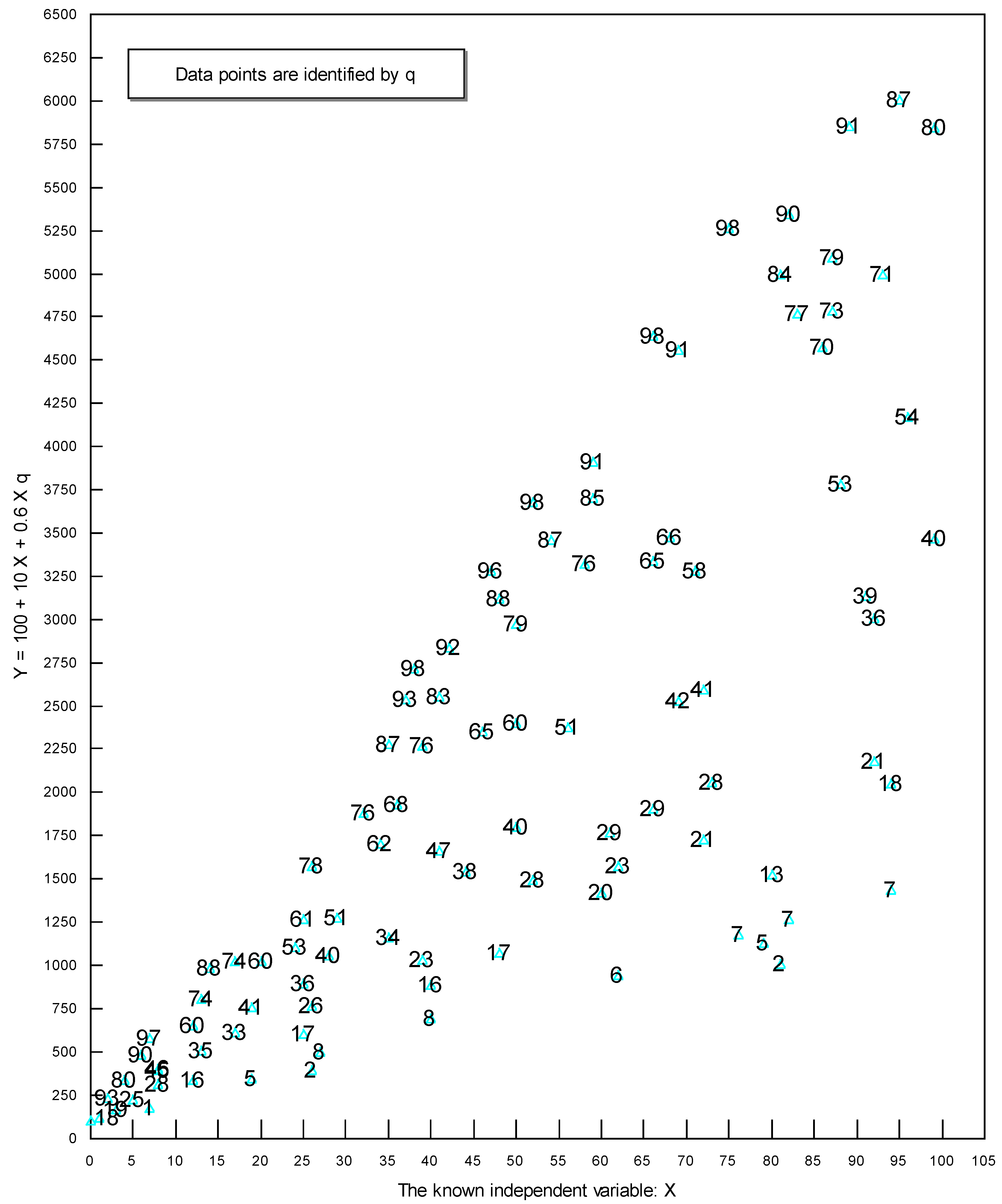
2. An Intuitive Explanation of the Analytical Technique Used
3. The Data and the Empirical Results

| dGDP/dM-1 | dCPI/dM-1 | |||||||||||||
|---|---|---|---|---|---|---|---|---|---|---|---|---|---|---|
| Japan | UK | USA | Euro 17 | Brazil | China | Russia | Japan | UK | US | Brazil | China | India | Russia | |
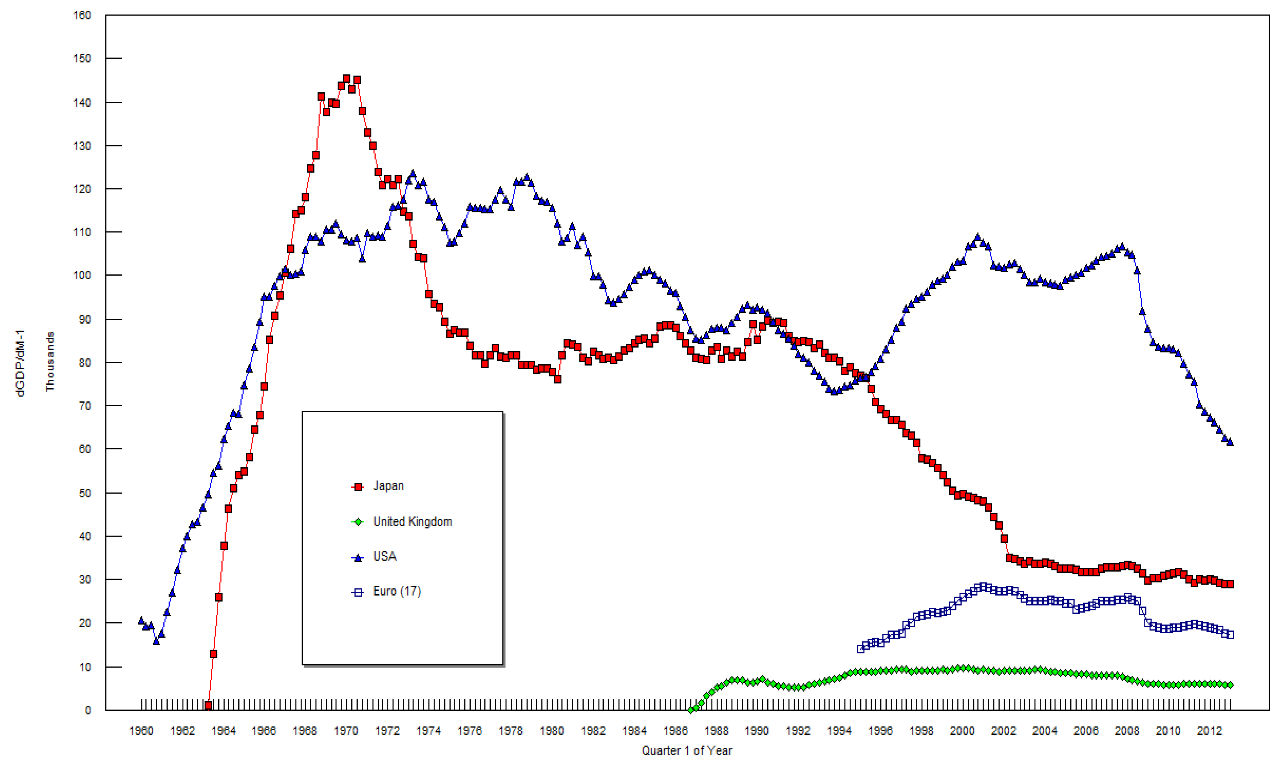
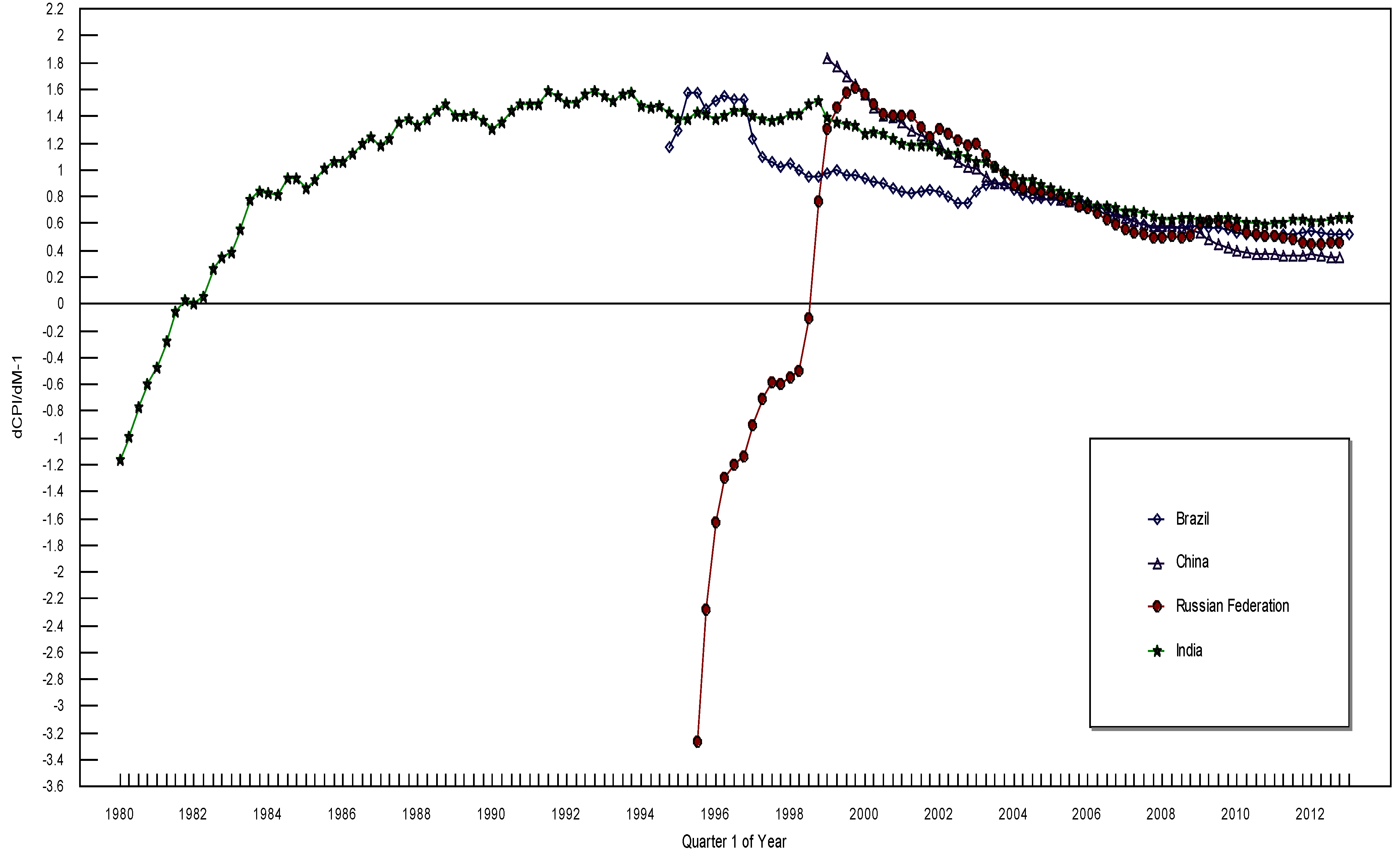
| Q1-1997 | 65,605 | 9416 | 89,489 | 17,589 | 13,525 | 0.435 | 0.594 | 0.747 | 1.228 | 1.402 | −0.907 | |||
| Q2-1997 | 63,753 | 9270 | 92,419 | 19,581 | 12,080 | 0.475 | 0.580 | 0.760 | 1.097 | 1.384 | −0.710 | |||
| Q3-1997 | 63,174 | 8714 | 93,583 | 20,154 | 12,124 | 0.467 | 0.533 | 0.761 | 1.065 | 1.368 | −0.590 | |||
| Q4-1997 | 61,541 | 8980 | 94,549 | 21,365 | 11,769 | 0.461 | 0.537 | 0.765 | 1.019 | 1.377 | −0.599 | |||
| Q1-1998 | 57,940 | 9046 | 95,144 | 21,894 | 10,940 | 0.437 | 0.520 | 0.763 | 1.050 | 1.416 | −0.553 | |||
| Q2-1998 | 57,571 | 9025 | 96,225 | 21,915 | 10,908 | 0.447 | 0.527 | 0.768 | 1.003 | 1.414 | −0.500 | |||
| Q3-1998 | 56,726 | 9117 | 97,983 | 22,458 | 10,376 | 0.427 | 0.520 | 0.773 | 0.946 | 1.483 | −0.112 | |||
| Q4-1998 | 55,757 | 9179 | 98,850 | 22,376 | 9983 | 0.436 | 0.518 | 0.765 | 0.948 | 1.520 | 0.761 | |||
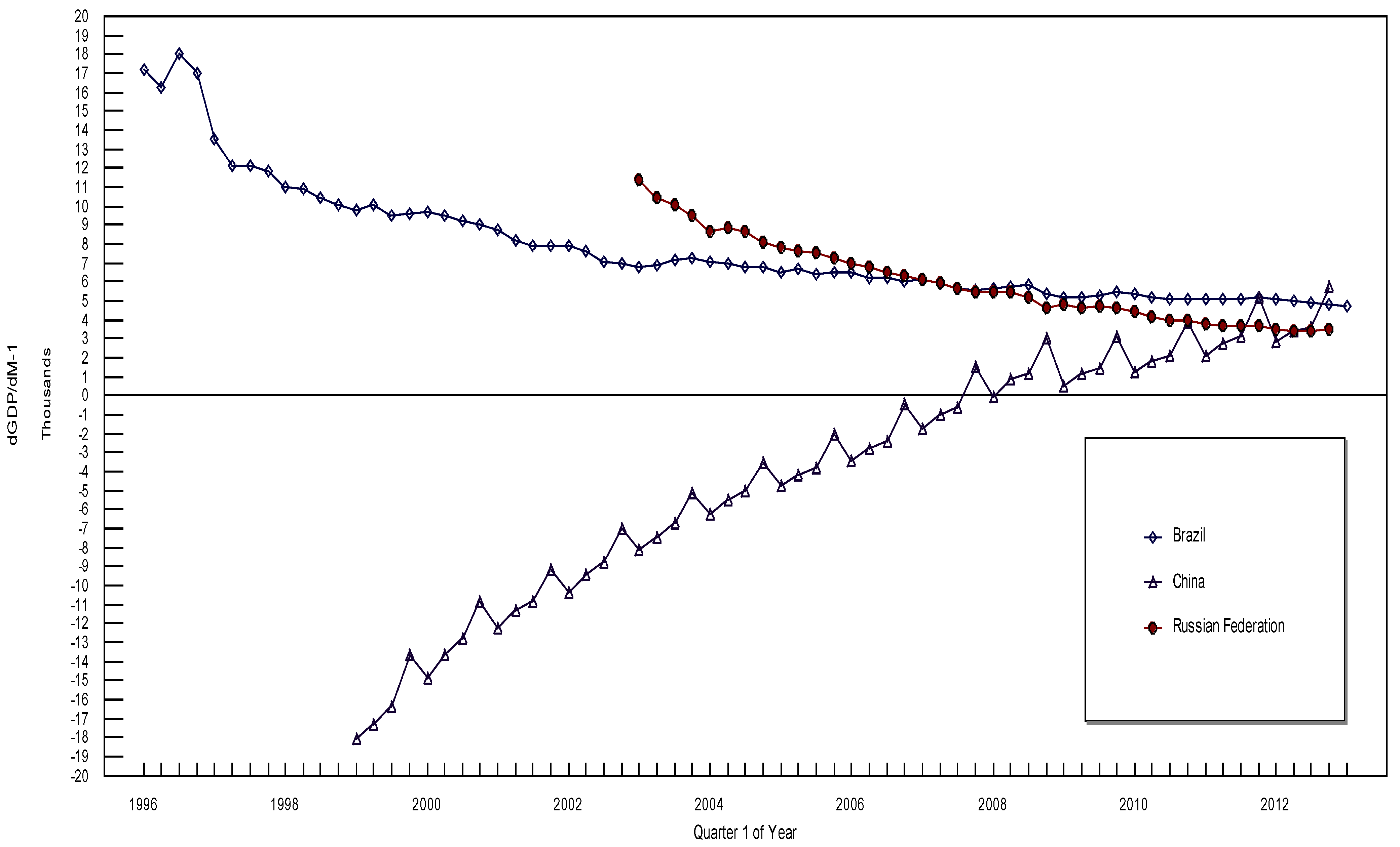
| Q1-1999 | 53,968 | 9224 | 99,450 | 22,452 | 9782 | −18,065 | 0.408 | 0.509 | 0.766 | 0.967 | 1.833 | 1.388 | 1.301 | |
| Q2-1999 | 52,356 | 9151 | 100,096 | 22,970 | 10,034 | −17,294 | 0.399 | 0.517 | 0.773 | 1.001 | 1.773 | 1.348 | 1.461 | |
| Q3-1999 | 50,476 | 9400 | 102,090 | 23,936 | 9514 | −16,386 | 0.381 | 0.497 | 0.782 | 0.965 | 1.702 | 1.341 | 1.579 | |
| Q4-1999 | 49,480 | 9576 | 103,205 | 25,183 | 9587 | −13,702 | 0.371 | 0.493 | 0.779 | 0.958 | 1.632 | 1.326 | 1.617 | |
| Q1-2000 | 49,489 | 9554 | 103,504 | 26,034 | 9659 | −14,883 | 0.353 | 0.471 | 0.789 | 0.940 | 1.562 | 1.264 | 1.568 | |
| Q2-2000 | 49,095 | 9557 | 106,643 | 26,817 | 9429 | −13,648 | 0.353 | 0.464 | 0.804 | 0.916 | 1.462 | 1.282 | 1.485 | |
| Q3-2000 | 48,731 | 9357 | 107,403 | 27,363 | 9187 | −12,842 | 0.348 | 0.449 | 0.817 | 0.900 | 1.401 | 1.265 | 1.416 | |
| Q4-2000 | 48,376 | 9180 | 109,023 | 28,193 | 8979 | −10,877 | 0.341 | 0.447 | 0.829 | 0.860 | 1.393 | 1.236 | 1.401 | |
| Q1-2001 | 47,980 | 9202 | 107,634 | 28,500 | 8706 | −12,222 | 0.329 | 0.423 | 0.833 | 0.842 | 1.357 | 1.197 | 1.402 | |
| Q2-2001 | 46,498 | 9082 | 106,810 | 28,033 | 8200 | −11,327 | 0.318 | 0.430 | 0.831 | 0.822 | 1.300 | 1.186 | 1.407 | |
| Q3-2001 | 44,503 | 9040 | 102,396 | 27,687 | 7882 | −10,815 | 0.305 | 0.421 | 0.801 | 0.838 | 1.252 | 1.189 | 1.317 | |
| Q4-2001 | 42,442 | 8900 | 102,083 | 27,376 | 7832 | −9144 | 0.286 | 0.412 | 0.792 | 0.854 | 1.242 | 1.185 | 1.250 | |
| Q1-2002 | 39,345 | 8998 | 101,664 | 27,165 | 7851 | −10,361 | 0.257 | 0.412 | 0.784 | 0.845 | 1.187 | 1.149 | 1.303 | |
| Q2-2002 | 35,078 | 9131 | 102,504 | 27,442 | 7602 | −9477 | 0.231 | 0.420 | 0.796 | 0.805 | 1.123 | 1.126 | 1.274 | |
| Q3-2002 | 34,593 | 9039 | 102,810 | 27,162 | 7066 | −8751 | 0.224 | 0.407 | 0.798 | 0.747 | 1.063 | 1.122 | 1.218 | |
| Q4-2002 | 34,042 | 9051 | 101,378 | 26,412 | 6900 | −7023 | 0.218 | 0.404 | 0.790 | 0.758 | 1.028 | 1.100 | 1.186 | |
| Q1-2003 | 33,533 | 9018 | 100,018 | 25,671 | 6777 | −8174 | 11,351 | 0.212 | 0.396 | 0.785 | 0.836 | 1.010 | 1.065 | 1.199 |
| Q2-2003 | 34,051 | 9119 | 98,577 | 25,056 | 6898 | −7498 | 10,409 | 0.217 | 0.396 | 0.769 | 0.886 | 0.955 | 1.055 | 1.110 |
| Q3-2003 | 33,509 | 9263 | 98,558 | 25,029 | 7129 | −6737 | 10,009 | 0.211 | 0.392 | 0.758 | 0.901 | 0.898 | 1.029 | 1.021 |
| Q4-2003 | 33,584 | 9240 | 99,158 | 25,207 | 7188 | −5145 | 9450 | 0.207 | 0.386 | 0.754 | 0.893 | 0.896 | 0.990 | 0.967 |
| Q1-2004 | 33788 | 9125 | 98,622 | 25,206 | 7019 | −6261 | 8639 | 0.203 | 0.373 | 0.753 | 0.847 | 0.885 | 0.950 | 0.883 |
| Q2-2004 | 33599 | 8907 | 98,144 | 25,239 | 6906 | −5486 | 8797 | 0.205 | 0.371 | 0.757 | 0.809 | 0.848 | 0.920 | 0.867 |
| Q3-2004 | 33040 | 8632 | 97,906 | 25,149 | 6771 | −5017 | 8620 | 0.201 | 0.360 | 0.751 | 0.794 | 0.830 | 0.920 | 0.856 |
| Q4-2004 | 32564 | 8524 | 97,588 | 24,930 | 6748 | −3549 | 8093 | 0.203 | 0.357 | 0.747 | 0.787 | 0.817 | 0.885 | 0.837 |
| Q1-2005 | 32397 | 8425 | 98,905 | 24,493 | 6497 | −4811 | 7760 | 0.195 | 0.350 | 0.753 | 0.779 | 0.809 | 0.869 | 0.820 |
| Q2-2005 | 32641 | 8441 | 99,620 | 24,411 | 6647 | −4227 | 7626 | 0.195 | 0.350 | 0.768 | 0.773 | 0.780 | 0.837 | 0.798 |
| Q3-2005 | 32204 | 8336 | 100,177 | 23,204 | 6400 | −3812 | 7462 | 0.189 | 0.344 | 0.777 | 0.771 | 0.760 | 0.813 | 0.764 |
| Q4-2005 | 31803 | 8314 | 100,722 | 23,295 | 6477 | −2043 | 7222 | 0.187 | 0.339 | 0.781 | 0.772 | 0.743 | 0.793 | 0.723 |
| Q1-2006 | 31770 | 8212 | 101,923 | 23,598 | 6455 | −3452 | 6986 | 0.185 | 0.331 | 0.783 | 0.751 | 0.735 | 0.749 | 0.717 |
| Q2-2006 | 31824 | 8051 | 102,450 | 24,012 | 6214 | −2776 | 6772 | 0.188 | 0.334 | 0.800 | 0.727 | 0.707 | 0.724 | 0.683 |
| Q3-2006 | 31827 | 7943 | 103,411 | 24,402 | 6150 | −2429 | 6439 | 0.191 | 0.334 | 0.814 | 0.698 | 0.673 | 0.729 | 0.625 |
| Q4-2006 | 32442 | 7910 | 104,225 | 24,952 | 5998 | −468 | 6292 | 0.189 | 0.332 | 0.804 | 0.666 | 0.650 | 0.716 | 0.586 |
| Q1-2007 | 32777 | 7944 | 104,488 | 25,008 | 6054 | −1783 | 6081 | 0.184 | 0.327 | 0.815 | 0.653 | 0.638 | 0.688 | 0.560 |
| Q2-2007 | 32826 | 7938 | 105,119 | 25,042 | 5876 | −1022 | 5957 | 0.188 | 0.326 | 0.831 | 0.622 | 0.616 | 0.688 | 0.536 |
| Q3-2007 | 32740 | 7806 | 106,279 | 25,244 | 5638 | −611 | 5611 | 0.190 | 0.312 | 0.836 | 0.591 | 0.598 | 0.683 | 0.516 |
| Q4-2007 | 32948 | 7629 | 106,644 | 25,459 | 5537 | 1473 | 5426 | 0.193 | 0.312 | 0.842 | 0.564 | 0.581 | 0.657 | 0.496 |
| Q1-2008 | 33278 | 7026 | 105,440 | 25,820 | 5615 | −58 | 5466 | 0.193 | 0.290 | 0.849 | 0.562 | 0.586 | 0.626 | 0.497 |
| Q2-2008 | 33006 | 6823 | 104,895 | 25,482 | 5736 | 845 | 5444 | 0.203 | 0.302 | 0.864 | 0.570 | 0.580 | 0.628 | 0.505 |
| Q3-2008 | 32613 | 6666 | 101,321 | 25,045 | 5851 | 1164 | 5142 | 0.212 | 0.317 | 0.857 | 0.574 | 0.569 | 0.642 | 0.497 |
| Q4-2008 | 31367 | 6280 | 91,842 | 22,916 | 5351 | 3013 | 4617 | 0.205 | 0.314 | 0.772 | 0.577 | 0.554 | 0.649 | 0.505 |
| Q1-2009 | 29723 | 5879 | 87,618 | 19,970 | 5165 | 510 | 4751 | 0.192 | 0.302 | 0.744 | 0.584 | 0.527 | 0.631 | 0.603 |
| Q2-2009 | 30230 | 5974 | 84,781 | 19,265 | 5158 | 1147 | 4632 | 0.192 | 0.316 | 0.730 | 0.574 | 0.477 | 0.615 | 0.615 |
| Q3-2009 | 30227 | 6035 | 83,568 | 18,986 | 5281 | 1400 | 4718 | 0.189 | 0.321 | 0.723 | 0.564 | 0.441 | 0.638 | 0.615 |
| Q4-2009 | 30829 | 5863 | 83,352 | 18,749 | 5390 | 3140 | 4636 | 0.183 | 0.315 | 0.714 | 0.551 | 0.420 | 0.644 | 0.593 |
| Q1-2010 | 31238 | 5740 | 83,384 | 18,637 | 5307 | 1201 | 4426 | 0.182 | 0.309 | 0.712 | 0.534 | 0.400 | 0.628 | 0.564 |
| Q2-2010 | 31298 | 5779 | 83,153 | 18,985 | 5186 | 1747 | 4150 | 0.182 | 0.316 | 0.710 | 0.519 | 0.384 | 0.608 | 0.536 |
| Q3-2010 | 31646 | 5869 | 82,331 | 19,059 | 5087 | 2055 | 3974 | 0.175 | 0.318 | 0.698 | 0.502 | 0.373 | 0.604 | 0.518 |
| Q4-2010 | 31220 | 5895 | 79,733 | 19,286 | 5058 | 3850 | 3948 | 0.175 | 0.331 | 0.673 | 0.500 | 0.366 | 0.595 | 0.507 |
| Q1-2011 | 30177 | 6036 | 77,221 | 19,619 | 5091 | 2044 | 3797 | 0.171 | 0.346 | 0.662 | 0.510 | 0.367 | 0.607 | 0.501 |
| Q2-2011 | 29196 | 5983 | 75,479 | 19,746 | 5087 | 2702 | 3655 | 0.169 | 0.354 | 0.657 | 0.517 | 0.359 | 0.611 | 0.494 |
| Q3-2011 | 29899 | 6005 | 70,439 | 19,637 | 5058 | 3141 | 3631 | 0.168 | 0.356 | 0.613 | 0.520 | 0.360 | 0.634 | 0.477 |
| Q4-2011 | 29667 | 5972 | 68,805 | 19,295 | 5118 | 5123 | 3636 | 0.164 | 0.362 | 0.591 | 0.534 | 0.357 | 0.632 | 0.460 |
| Q1-2012 | 29913 | 6031 | 67,393 | 19,063 | 5089 | 2784 | 3509 | 0.165 | 0.369 | 0.581 | 0.539 | 0.367 | 0.615 | 0.449 |
| Q2-2012 | 29662 | 5948 | 66,258 | 18,823 | 4952 | 3401 | 3419 | 0.166 | 0.373 | 0.575 | 0.529 | 0.358 | 0.623 | 0.447 |
| Q3-2012 | 29065 | 5932 | 64,538 | 18,296 | 4858 | 3594 | 3417 | 0.159 | 0.367 | 0.556 | 0.522 | 0.350 | 0.633 | 0.453 |
| Q4-2012 | 28885 | 5788 | 62,485 | 17,582 | 4791 | 5686 | 3475 | 0.157 | 0.370 | 0.538 | 0.520 | 0.345 | 0.644 | 0.453 |
| Q1-2013 | 28824 | 5655 | 61,870 | 17,229 | 4704 | 0.154 | 0.362 | 0.533 | 0.518 | 0.643 | ||||


4. Conclusions
Acknowledgments
Conflicts of Interest
References
- J. Mead, and J. Hilsenrath. “Banks Rush to Ease Supply of Money.” Wall Street Journal, 14 May 2013, A7. [Google Scholar]
- P. Dvorak, and E. Warnock. “Suffering Japan Rolls Dice on New Era of Easy Money.” Wall Street Journal, 21 March 2013, A1–A12. [Google Scholar]
- A. Frangos. “Asia Wrestles with a Flood of Cash.” Wall Street Journal, 9 May 2013, C1–C4. [Google Scholar]
- E. McCarthy, P. Natarajan, and K. Inagaki. “Japan Triggers a Shift to Emerging Markets.” Wall Street Journal, 15 April 2013, C1–C2. [Google Scholar]
- J.E. Leightner. The Changing Effectiveness of Key Policy Tools in Thailand. Singapore: Institute of Southeast Asian Studies for East Asian Development Network, 2002. [Google Scholar]
- J.E. Leightner, and T. Inoue. “Tackling the omitted variables problem without the strong assumptions of proxies.” Eur. J. Oper. Res. 178 (2007): 819–840. [Google Scholar] [CrossRef]
- T. Inoue, P. Lafaye de Micheaux, and J.E. Leightner. “Several related solutions to the omitted variables problem.” 2013, unpublished work. [Google Scholar]
- J.K. Abbott, and H.A. Klaiber. “An embarrassment of riches: Confronting omitted variable bias and multiscale capitalization in hedonic price models.” Rev. Econ. Stat. 93 (2011): 1331–1342. [Google Scholar] [CrossRef]
- J.D. Angrist, and A.B. Krueger. “Instrumental variables and the search for identification: From supply and demand to natural experiments.” J. Econ. Perspect. 15 (2001): 69–85. [Google Scholar] [CrossRef]
- S.E. Black, and L.M. Lynch. “How to compete: The impact of workplace practices and information technology on productivity.” Rev. Econ. Stat. 83 (2001): 434–445. [Google Scholar] [CrossRef]
- C.A. Botosan, and M.A. Plumlee. “A re-examination of disclosure level and the expected cost of equity capital.” J. Account. Res. 40 (2002): 21–40. [Google Scholar]
- S.R. Cellini. “Causal inference and omitted variable bias in financial aid research: Assessing solutions.” Rev. High. Educ. 31 (2008): 329–354. [Google Scholar] [CrossRef]
- T.A. DiPrete, and M. Gangl. “Assessing Bias in the Estimation of Causal Effects: Rosenbaum Bounds on Matching Estimators and Instrumental Estimation with Imperfect Instruments.” Available online: http://www.wjh.harvard.edu/~cwinship/cfa_papers/HBprop_021204.pdf (accessed on 20 March 2013).
- A.L. Harris, and K. Robinson. “Schooling behaviors or prior skills? A cautionary tale of omitted variable bias within oppositional culture theory.” Sociol. Educ. 80 (2007): 139–157. [Google Scholar] [CrossRef]
- D.B. Mustard. “Reexamining criminal behavior: The importance of omitted variable bias.” Rev. Econ. Stat. 85 (2003): 205–211. [Google Scholar] [CrossRef]
- R.K. Pace, and J.P. LeSage. “Omitted Variable Biases of OLS and Spatial Lag Models.” In Progress in Spatial Analysis: Advances in Spatial Science. Berlin, Germany: Springer-Verlag Berlin Heidelberg, 2010. [Google Scholar]
- R.W. Paterson, and K.J. Boyle. “Out of sight, out of mind? Using GIS to incorporate visibility in hedonic property value models.” Land Econ. 78 (2002): 417–425. [Google Scholar] [CrossRef]
- R.M. Scheffler, T.T. Brown, and J.K. Rice. “The role of social capital in reducing non-specific psychological distress: The importance of controlling for omitted variable bias.” Soc. Sci. Med. 65 (2007): 842–854. [Google Scholar] [CrossRef]
- D.N. Sessions, and L.K. Stevans. “Investigating omitted variable bias in regression parameter estimation: A genetic algorithm approach.” Comput. Stat. Data Anal. 50 (2006): 2835–2854. [Google Scholar] [CrossRef]
- S.C. Streams, and E.C. Norton. “Time to include time to death? The future of health care expenditure predictions.” Health Econ. 13 (2004): 315–327. [Google Scholar] [CrossRef]
- P.A.V.B. Swamy, I.L. Chang, J.S. Mehta, and G.S. Tavlas. “Correcting for omitted-variable and measurement-error bias in autoregressive model estimation with panel data.” Comput. Econ. 22 (2003): 225–253. [Google Scholar] [CrossRef]
- J. Branson, and C.A. Knox Lovell. “Taxation and Economic Growth in New Zealand.” In Taxation and the Limits of Government. Edited by G.W. Scully and P.J. Caragata. Boston, MA, USA: Kluwer Academic, 2000, pp. 37–88. [Google Scholar]
- J.E. Leightner. “Omitted variables and how the Chinese yuan affects other Asian currencies.” Int. J. Contemp. Math. Sci. 3 (2008): 645–666. [Google Scholar]
- J.E. Leightner, and T. Inoue. “Solving the omitted variables problem of regression analysis using the relative vertical position of observations.” Adv. Decis. Sci. 2012, 2012, p. 728980. Available online: http://www.hindawi.com/journals/ads/2012/728980/ (accessed on 11 March 2013).
- J.E. Leightner, and T. Inoue. “Is China replacing the USA as an engine for global growth? ” Int. Econ. Financ. J. 7 (2012): 55–77. [Google Scholar]
- J.E. Leightner, and T. Inoue. “Negative fiscal multipliers exceed positive multipliers during Japanese deflation.” Appl. Econ. Lett. 16 (2009): 1523–1527. [Google Scholar] [CrossRef]
- J.E. Leightner, and T. Inoue. “Capturing climate’s effect on pollution abatement with an improved solution to the omitted variables problem.” Eur. J. Oper. Res. 191 (2008): 539–556. [Google Scholar]
- J.E. Leightner, and T. Inoue. “The effect of the Chinese yuan on other Asian Currencies during the 1997–1998 Asian Crisis.” Int. J. Econ. Issues 1 (2008): 11–24. [Google Scholar]
- J.E. Leightner. “Chinese Overtrading.” In Two Asias: The Emerging Postcrisis Divide. Edited by S. Rosefielde, M. Kuboniwa and S. Mizobata. Singapore: World Scientific Publishers, 2011. [Google Scholar]
- J.E. Leightner. “Fiscal stimulus for the USA in the current financial crisis: What does 1930–2008 tell us? ” Appl. Econ. Lett. 18 (2011): 539–549. [Google Scholar] [CrossRef]
- J.E. Leightner. “Are the forces that cause China’s trade surplus with the USA good? ” J. Chin. Econ. Foreign Trade Stud. 3 (2010): 43–53. [Google Scholar] [CrossRef]
- J.E. Leightner. “China’s fiscal stimulus package for the current international crisis, what does 1996–2006 tell us? ” Front. Econ. China 5 (2010): 1–24. [Google Scholar] [CrossRef]
- J.E. Leightner. “How China’s holdings of foreign reserves affect the value of the US dollar in Europe and Asia.” China World Econ. 18 (2010): 24–39. [Google Scholar]
- J.E. Leightner. “Omitted variables, confidence intervals, and the productivity of exchange rates.” Pac. Econ. Rev. 12 (2007): 15–45. [Google Scholar] [CrossRef]
- J.E. Leightner. “Fight deflation with deflation, not with monetary policy.” Jpn. Econ. Transl. Stud. 33 (2005): 67–93. [Google Scholar]
- J.E. Leightner. “The productivity of government spending in Asia: 1983–2000.” J. Product. Anal. 23 (2005): 33–46. [Google Scholar] [CrossRef]
- B. Casselman. “Cautious Companies Stockpile Cash.” Wall Street Journal, 7 December 2012, A2. [Google Scholar]
- E. Chasan. “Lots of Cash, Few Alternatives: Company Funds Stay Put at Banks Even after Unlimited Deposit Insurance Expires.” Wall Street Journal, 23 April 2013, B6. [Google Scholar]
- S. Fidler. “Firms’ Cash Hoarding Stunts Europe.” Wall Street Journal, 24–25 March 2012, A10. [Google Scholar]
- T. Gara. “S&P: U.S. Companies Underinvest by Billions.” Wall Street Journal, 12 December 2012, B6. [Google Scholar]
- J. Hilsenrath, and R. Simon. “Penitent Debtors Hobble Recovery in U.S.” Wall Street Journal, 22–23 October 2011, A1–A14. [Google Scholar]
- V. Monga. “Companies’ $2 Trillion Conundrum.” Wall Street Journal, 5 October 2011, B5. [Google Scholar]
- R. Sidel. “Wads of Cash Squeeze Bank Margins.” Wall Street Journal, 11 January 2013, C1. [Google Scholar]
- J.M. Keynes. The General Theory of Employment, Interest and Money. London, UK: MacMillan, 2007. [Google Scholar]
© 2013 by the authors; licensee MDPI, Basel, Switzerland. This article is an open access article distributed under the terms and conditions of the Creative Commons Attribution license (http://creativecommons.org/licenses/by/3.0/).
Share and Cite
Leightner, J.E. The Changing Effectiveness of Monetary Policy. Economies 2013, 1, 49-64. https://doi.org/10.3390/economies1030049
Leightner JE. The Changing Effectiveness of Monetary Policy. Economies. 2013; 1(3):49-64. https://doi.org/10.3390/economies1030049
Chicago/Turabian StyleLeightner, Jonathan E. 2013. "The Changing Effectiveness of Monetary Policy" Economies 1, no. 3: 49-64. https://doi.org/10.3390/economies1030049
APA StyleLeightner, J. E. (2013). The Changing Effectiveness of Monetary Policy. Economies, 1(3), 49-64. https://doi.org/10.3390/economies1030049