Overview of the Application of Physically Informed Neural Networks to the Problems of Nonlinear Fluid Flow in Porous Media

Abstract

To describe unsteady multiphase flows in porous media, it is important to consider the non-Newtonian properties of fluids by including rheological laws in the hydrodynamic model. This leads to the formation of a nonlinear system of partial differential equations. To solve this direct problem, it is necessary to linearize the equation system. Algorithm construction for inverse problem solution is problematic since the numerical solution is unstable. The application of implicit methods is reduced to matrix equations with a high rank of the coefficient matrix, which requires significant computational resources. The authors of this paper investigated the possibility of parameterized function (physics-informed neural networks) application to solve direct and inverse problems of non-Newtonian fluid flows in porous media. The results of laboratory experiments to process core samples and field data from a real oil field were selected as examples of application of this method. Due to the lack of analytical solutions, the results obtained via the finite difference method and via real experiments were proposed for validation.

1. Introduction

A feature of unsteady flow problems is a description of hydrodynamic processes by a system of partial differential equations (PDEs). The numerical solution of such systems involves the application of complex integration methods, even for the one-dimensional case [1,2]. Accounting for the flow multidimensionality, the multiphase nature of the filtered fluids and the necessity of phase interaction considerations (taking into account the ongoing phase transitions and chemical reactions) significantly complicates the system [3]. Paper [4] provides an extensive overview of modern approaches to integrating systems of PDEs, including describing fluid flow in porous media with mass flows between phases. In classical approaches to integrating nonlinear systems, the finite difference method, the finite element method, the finite volume method and their various modifications are applied to solve both direct and inverse problems. As a rule, high-resolution structured grids are applied in calculations, which leads to a large amount of calculations. The construction of non-structured grids, for example, based on Voronoy diagrams, allows for a more detailed consideration of the flow geometry and increases the accuracy of calculations; however, they require the construction of special algorithms and do not eliminate the problem of the large amount of calculations [5,6].

Hydrodynamic modeling aims to solve the direct problem of non-steady fluid flow with specified reservoir properties (porosity, permeability and the physical properties of saturated reservoir phases) based on the data obtained from geological studies and well exploration analyses. The main goal is to obtain the time dependencies of the flow process parameters (density, viscosity, pressure, temperature, etc.).

To predict further reserve recovery developments (which last for decades in some fields), it is necessary to adjust the input data sets, determining the properties of the simulated saturated reservoir system at all stages of deposit development. In practice, this process is carried out by conducting well hydrodynamic studies and determining the current reservoir properties by analyzing changes in the pressure and temperature sensors obtained from sensors during start/stop of the well. Mathematically, the flow theory inverse problem solution is considered, which could be carried out in three ways. The classical (first) approach includes an iterative way to solve a conservation equation system written in finite-difference form with the initial and boundary conditions [7,8]. The main disadvantage of this method is that it uses large amounts of computing resources, especially for multidimensional flows.

The second approach applies basic machine learning (ML) algorithms. It is based on the analysis of the variety of direct problem solutions. In fact, it is similar to the approach of choosing a “suitable” solution within the hydrodynamic function domain based on “expert” assessments of previous options. The problem is solved by minimizing the quality functional between the defined and given parameters (hydrodynamic, filtration, capacitive), for example, according to the least squares criterion [9]. The significant disadvantage of ML algorithm implementation is the availability of a substantial “training” data set (actual data or previously obtained solutions). This is impossible at the initial stage of a field development or during modification of an already existing field development scheme. Furthermore, when the details of the layer are not fully understood, error variance may arise, and its magnitude is strongly influenced by the choice of the deviation functional, the training data set content, and the choice of “expert” constraints.

The third method proposed in [4,10] is the physics-informed neural network (PINN), which considers (opposite to ML) the physics of the process, since the loss function contains a form of differential equations (for example, mass, momentum and energy conservation laws). The advantage of PINN application to non-steady flow problems is the uniformity of the algorithm when applied to numerical simulations of direct and inverse problems.

At the moment, there are many approaches based on the PINN concept. For example, there are variational PINNs (hp-VPINNs) [11], which use a variational concept to construct the loss functional, and conservative PINNs [12], where additional terms to the loss function are included, “penalizing” for the failure of the basic conservation laws. A conservative PINN is capable of increasing the accuracy of the solution, but it is only applicable to certain types of systems (conservation laws). In [13], the X-PINN model was proposed, which expands the applicability of conservative PINNs by overcoming the equation type limitations. The authors of [14] propose applying an adaptable algorithm for generating a training data set to improve the accuracy of such models. They consider the distribution of errors (according to the loss function) and increase the data set size in the vicinity of large errors. Since the initial data of the problem often contain some noise (a recognized fact in oil and gas problems), it is proposed to apply a Bayesian physics-informed neural network (B-PINN) to obtain more accurate solutions [15]. Improving the accuracy of the solution is achieved due to their ability to avoid overtraining.

PINN algorithms have been successfully applied to solve practical problems in fluid mechanics, including in porous media. For example, in [16], the problems of shock wave propagation are considered, which are popular in computational mechanics. In [17], a PINN is applied to consider the classical formulation of two-phase flow according to Darcy’s law [18] with the application of convolutional physics-informed neural networks. It is difficult to consistently solve a set of different equations using PINNs, as for each equation, it is necessary to manually redefine various program blocks (for example, the loss function). However, solvers for PINN automation are already being developed [19,20].

In most of the current tasks for developing hard-to-recover hydrocarbon reserves, it is important to consider the rheological properties of the fluids. Therefore, the PDE system becomes nonlinear. In this paper, the possibility of using PINN-based methods to obtain flow problem solutions which consider the description of the nonlinearities of the viscous properties of fluids is analyzed.

This paper is organized as follows: In Section 2, the mathematical formulation of the proposed algorithm for solving the considered equation system type is consistently presented. Section 3 contains the results of the formulated error function application to solving problems of nonlinear liquid filtration in a porous medium, validated by comparing the calculations with data obtained from one-dimensional physical experiments of two characteristic sizes of the analyzed object: several centimeters, using the example of core samples (Section 3.1), and hundreds of meters, based on field measurements of indicators at a well (Section 3.2).

2. Mathematical Approach

In parameterized model applications for solving differential equations, the solution obtaining problem is reduced to the minimization problem. Consider a differential equation depending on p independent variables $x=(x^1,x^2,\dots ,x^p)\in \mathrm{\Omega }\subset {\mathbb{R}}^p$ written in operator mode and defined on domain $\mathrm{\Omega }$ with boundaries $\partial \mathrm{\Omega }$:

$$\begin{array}{c}Lu=f{|}_{\mathrm{\Omega }}bu=g{|}_{\partial \mathrm{\Omega }}.\end{array}$$

(1)

In Equation (1), the differential operator L, boundary operator b and random functions f and g are known and hence the boundary value problem is correct. The problem of obtaining Equation (1)’s solution using the Cauchy–Schwarz equation is reduced to the minimization problem [20]:

$$\tilde{u}=\arg \underset{u}{min}\left|\right|Lu-{f\left|\right|}_D.$$

(2)

Here, D is the Sobolev space induced from the space of basis functions $C^{\infty }\left(\mathrm{\Omega }\right)$ with compact support.

In the next step, it is necessary to move from the analytical formulation of the minimization problem to the numerical one. Most numerical methods assume that the solution field is in a finite discrete subset of $\mathrm{\Omega }$ in the form of a grid function (for simplicity and without generality loss, consider the case of $\mathrm{\Omega }\in R^2$). Further, for an equation depending on two variables, the following functional representation is defined:

$$\begin{array}{c}\overline{u}=\{u(x^{\left(i\right)},t^{\left(i\right)}),i=1,2\},\\ \forall i(x^{\left(i\right)},t^{\left(i\right)})\in \mathrm{\Omega }.\end{array}$$

(3)

Without generality loss, we assume that the discretization of the field $X=\{x^{\left(i\right)},t^{\left(i\right)}\}\subset \mathrm{\Omega }$ is fixed in the process of solving the differential equation. The minimization problem of finding the solution field of Equation (1) can be formulated as:

$$\underset{\overline{u}}{min}{\lambda }_r\left|\right|L\overline{u}-{f\left|\right|}_2+{\lambda }_b\left|\right|b\overline{u}-g{\left|\right|}_2.$$

(4)

As a rule, $l_2$ norms are applied in the implementation of this approach. However, it can be assumed that the solution of the equation can be more accurate when the norms associated with the original Sobolev space are applied. The parameters ${\lambda }_r$ and ${\lambda }_b$ act as regularization coefficients, and can be both functions and constant coefficients. In [21], it is proposed to use the neural tangent kernel (NTK) to ensure better algorithm convergence by evaluating the parameters ${\lambda }_r$ and ${\lambda }_b$ in terms of their inverse contribution to the variance, which is calculated using the NTK eigenvalues. The parameters ${\lambda }_r$ and ${\lambda }_b$ are considered as constant and positive in this research. Since the solution of the equation is unknown, numerical differentiation methods are applied. They are implemented in the deep learning library Pytorch to obtain the values of $L\overline{u}$ for the solution and approximation at a specific iterative step. In practice, the differential $\overline{L}$ and boundary $\overline{b}$ operators are also approximations of continuous L and b operators with some error. Therefore, the minimization functional for solving a direct problem can be formulated as follows:

$$\underset{\overline{u}}{min}\left[{\lambda }_r\left|\right|\overline{L}\overline{u}-{f\left|\right|}_2+{\lambda }_b\left|\right|\overline{b}\overline{u}-g{\left|\right|}_2\right]{|}_X.$$

(5)

In Equation (5), the differential $\overline{L}$ and boundary $\overline{b}$ operators are numerical discretizations of differential operators, and the field X represents a grid covering the solution domain $\mathrm{\Omega }$. When solving the inverse problem, the additive component responsible for the convergence of the equation solution to the value set from physical observations should be added to Equation (5); further, the functional for solving the direct and inverse problems will be written as follows:

$$\underset{\overline{u}}{min}\left[{\lambda }_r\left|\right|\overline{L}\overline{u}-{f\left|\right|}_2+{\lambda }_b\left|\right|\overline{b}\overline{u}-g{\left|\right|}_2\right]{|}_X+{\lambda }_d\left|\right|\overline{u}-data{\left|\right|}_2{|}_Z.$$

(6)

In Equation (6), the $Z\subset \mathrm{\Omega }$ field represents a set of points where the values of the desired function are measured. The parameter ${\lambda }_d$ is the regularization coefficient responsible for the “degree of importance” of the last component for the optimization algorithm. For the numerical implementation of the minimization algorithm, it is necessary to determine the parameterized model itself, which approximates the values of the desired solution. In physical-based algorithms, neural networks are applied with different architectures. The authors of this paper applied a multilayer neural network, where $\overline{u}(x,t;\mathrm{\Theta })$ was used as a function, $R^p\to R$ and $\mathrm{\Theta }=\{{\theta }_1,\dots {\theta }_N\}$ is the set of neural network parameters, which is determined from the minimization problem of the following functional:

$$\begin{array}{c}\underset{\mathrm{\Theta }}{min}\left[{\lambda }_r\left|\right|\overline{L}\overline{u}(x,t;\mathrm{\Theta })-{f\left|\right|}_2+{\lambda }_b\left|\right|\overline{b}\overline{u}(x,t;\mathrm{\Theta })-g{\left|\right|}_2\right]{|}_X+\\ {\lambda }_d\left|\right|\overline{u}(x,t;\mathrm{\Theta })-data{\left|\right|}_2{|}_Z.\end{array}$$

(7)

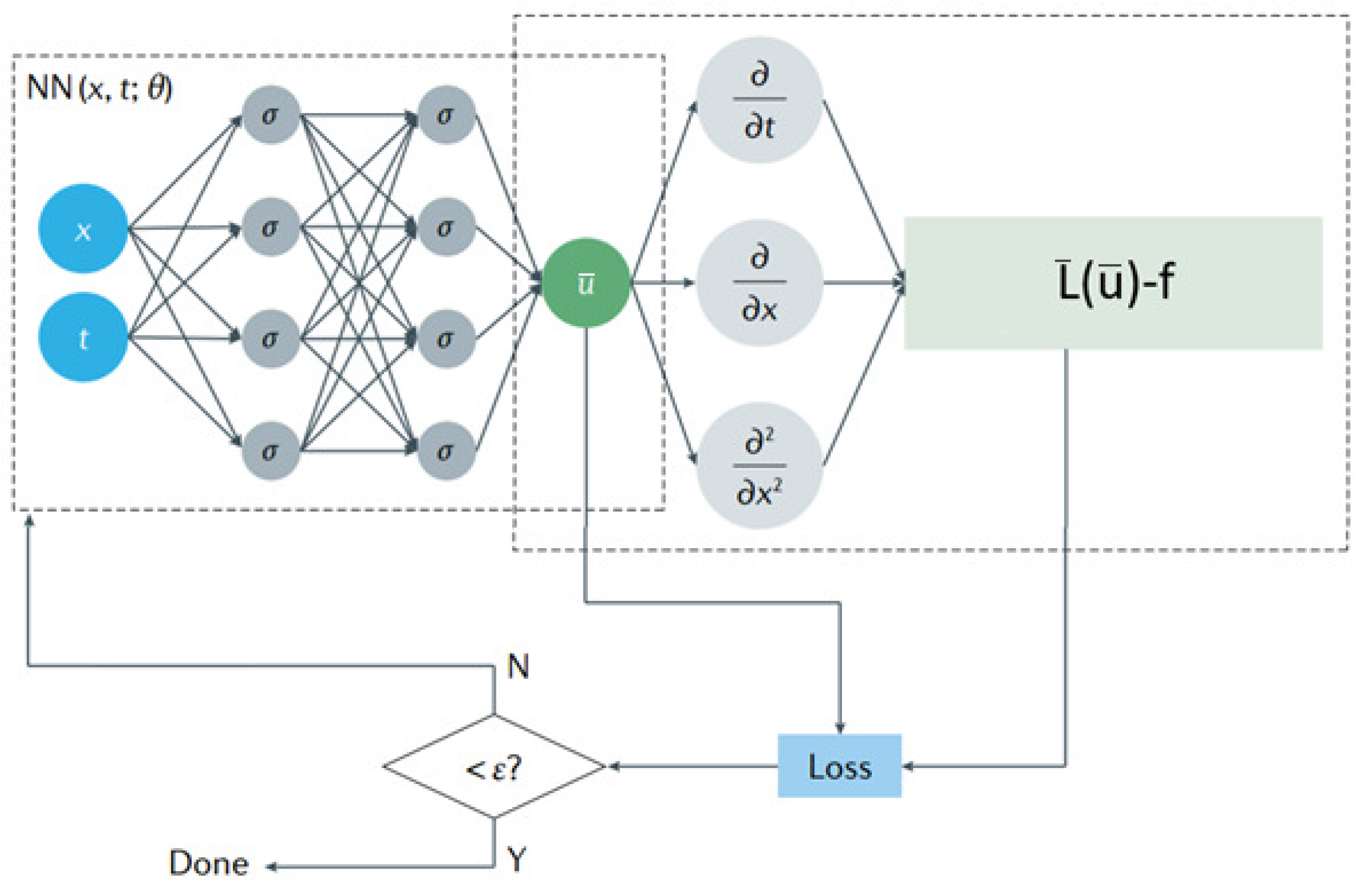
Figure 1 shows the schematic algorithm for solving the differential equation using a parameterized model (neural network).

3. Flow Theory Direct and Inverse Problem Solution Results

The flow velocities are low during fluid filtration through porous media, and the velocity is often described by Darcy’s law (linear dependence of the velocity vector on the pressure gradient) [22]. Nonlinear flow equations are used, as a rule, only for highly viscous fluids, for which non-Newtonian properties are established in the laboratory via rotary viscometers. It was noticed (in dynamic experiments on core samples) that the nonlinear behavior of the fluid also occurs in non-stationary modes in the area of small pressure gradients, including Newtonian liquids [23]. At the same time, it is important to establish the type of dependence of viscosity on the pressure gradient, taking into account the experimental results. To simulate a physical experiment on a real core [23], a system of isothermal flow equations on a space-time grid $(x,t)\in [0,L]\times [0,T]\subset \mathrm{\Omega }$ was considered, including the fluid mass conservation law (oil), the flow velocity equation with apparent viscosity [8], the elastic matrix porosity change equation, and the fluid state equation:

$$\begin{array}{c}\left\{\begin{array}{c}\frac{\partial \left(\rho m\right)}{\partial t}+div\left(\rho \overrightarrow{w}\right)=0,\hfill \\ \overrightarrow{w}=-\frac{k}{\mu }\nabla p,\hfill \\ \mu =\frac{{\mu }_H-{\mu }_L}{1+expB\left(\right|\nabla p|-G)}+{\mu }_L,\hfill \\ m=m_0+{\beta }_s(p-p_0),\hfill \\ \rho ={\rho }_0(1+{\beta }_0(p-p_0)).\hfill \end{array}\right.\end{array}$$

(8)

Here, m and k are, respectively, the porosity of the sample and its permeability (k is set according to the core study data and depends on porosity) and $\rho$ is the density of the fluid depending on the pressure p; the viscosity function $\mu$ depending on the pressure gradient is used in the form proposed in [8]. The unknown constants B and G define the form of the rheological curve of the drop in oil viscosity from the initial high value ${\mu }_H$ (also unknown) to the final value ${\mu }_L$ recorded on a rotary viscometer; $m_0$ and ${\rho }_0$, respectively, are the sample porosity and the oil density at initial pressure $p_0$; ${\beta }_0$ and ${\beta }_s$ are the compressibility coefficients of the porous matrix and oil, respectively; and $\overrightarrow{w}$ is the flow velocity vector ($\overrightarrow{w}=\overrightarrow{v}m$) of the oil phase.

Due to the small size of the core sample, the flow can be simulated in a one-dimensional formulation. Further, after substituting the flow velocity law into the mass conservation equation and non-dimensioning ($\overline{x}=\frac{x}{L}$, $\overline{t}=\frac{t}{T}$, $\overline{p}=\frac{p}{p_0}$) the system is written as follows:

$$\begin{array}{c}\left\{\begin{array}{c}\frac{{\beta }_{*}}{T}\frac{\partial \overline{p}}{\partial \overline{t}}-\frac{1}{L^2}\frac{\partial }{\partial \overline{x}}\left(\frac{k}{\mu }\frac{\partial \overline{p}}{\partial \overline{x}}\right)=0,\hfill \\ \mu =\frac{{\mu }_H-{\mu }_L}{1+exp\frac{B{P}_0}{L}\left(\right|\frac{\partial \overline{p}}{\partial x}|-G)}+{\mu }_L.\hfill \end{array}\right.\\ (\overline{x},\overline{t})\in [0,1]\times [0,1]\subset \overline{\mathrm{\Omega }}\end{array}$$

(9)

The coefficient ${\beta }_{*}={\beta }_0+{\beta }_s{m}_0$ sets the compressibility properties of the core sample and fluid in a complex way. System 9 is solved considering the initial and boundary conditions:

$$\begin{array}{c}\left\{\begin{array}{c}\frac{\partial \overline{p}}{\partial \overline{x}}{|}_{(0,\overline{t})}=\frac{q\mu L}{k{p}_0},\hfill \\ \overline{p}(\overline{x},0)=1,\hfill \\ \overline{p}(1,\overline{t})=1.\hfill \end{array}\right.\end{array}$$

(10)

where q is the oil flow rate related to the area of the inlet area.

3.1. Laboratory Experiment Interpretation

To assess the quality of solutions obtained via the proposed method, a direct test task (a series of launches) was initially solved and compared with solutions obtained by the finite difference method. The expression $rRMSE=\sqrt{\frac{\left|\right|p_{fd}-p_{pinn}{\left|\right|}_2^2}{\left|\right|p_{fd}{\left|\right|}_2^2}}$ was chosen as a quality assessment metric, where $p_{fd}$ and $p_{pinn}$ are solutions obtained by the finite difference method and using a PINN, respectively. The loss function, defined in this case based on Equation (7) (for ${\lambda }_d=0$), is represented as:

$$\underset{\mathrm{\Theta }}{min}{\lambda }_r\left[\left|\right|{\mathcal{L}}_r{\left|\right|}_2+{\lambda }_b\left|\right|{\mathcal{L}}_b{\left|\right|}_2\right]{|}_X.$$

(11)

This function is defined on a space-time grid X. ${\mathcal{L}}_b$ is defined by a vector with components in the form of residuals according to initial and boundary conditions:

$$\left\{\begin{array}{c}{\mathcal{L}}_r=\frac{{\beta }_{*}}{T}\frac{\partial \overline{p}}{\partial \overline{t}}-\frac{1}{L^2}\frac{\partial }{\partial \overline{x}}\left(\frac{k}{\mu }\frac{\partial \overline{p}}{\partial \overline{x}}\right),\hfill \\ {\mathcal{L}}_b=\left[\frac{\partial \overline{p}}{\partial \overline{x}}{|}_{(0,\overline{t})}-\frac{q\mu L}{k{p}_0},\overline{p}(\overline{x},0)-1,\overline{p}(1,\overline{t})-1\right].\hfill \end{array}\right.$$

(12)

A fully connected neural network with four hidden layers of 100 neurons and a hyperbolic tangent as an activation function was applied; the weight coefficients in the loss function were set by the constants ${\lambda }_r=10$ and ${\lambda }_b=100$. The Adam (Adaptive Moment Estimation) [24] optimization algorithm was used in numerical experiments with an optimization step of lr = 1 × 10⁻³, and the number of iterations was epoch = 35,000. $\overline{\mathrm{\Omega }}$ was covered by the uniform square grid X, which consists of $(N_x,N_t)=(50,50)$ collocation points. The input data of the problem are shown in

Table 1. The input parameters for solving the direct problem.

$p_0=25\mathrm{MPa}$	${\beta }_{*}={10}^{-9}{\mathrm{Pa}}^{-1}$	$k=2.5\mathrm{mD}$
$q=0.1\frac{\mathrm{m}}{\mathrm{day}}$	${\mu }_H=13.6\mathrm{mPa}\mathrm{s}$	${\mu }_L=4.62\mathrm{mPa}\mathrm{s}$
$G=0.025\frac{\mathrm{MPa}}{\mathrm{m}}$	$B=0.8\times {10}^{-3}\frac{\mathrm{m}}{\mathrm{Pa}}$	$T=1\mathrm{day}$

.

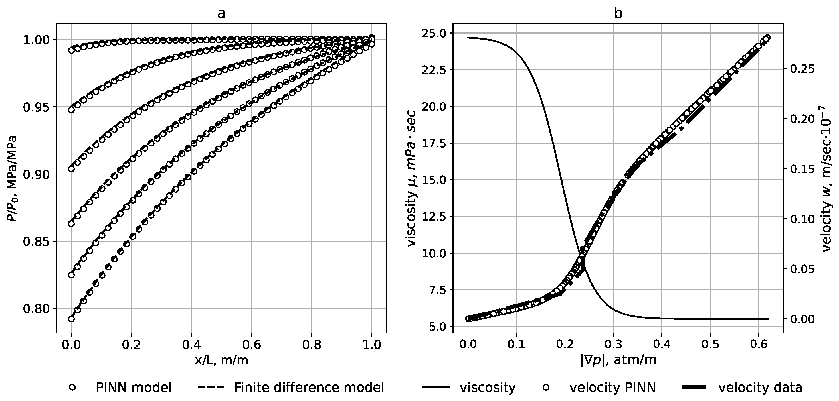
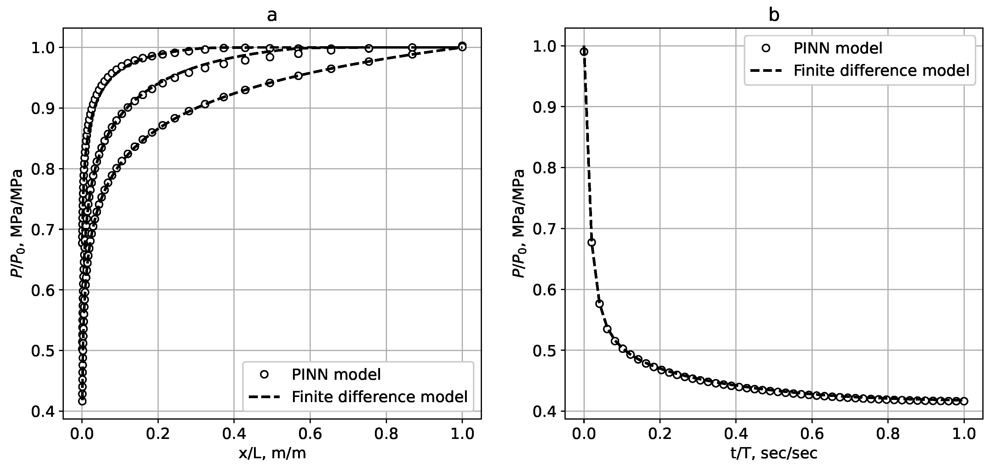
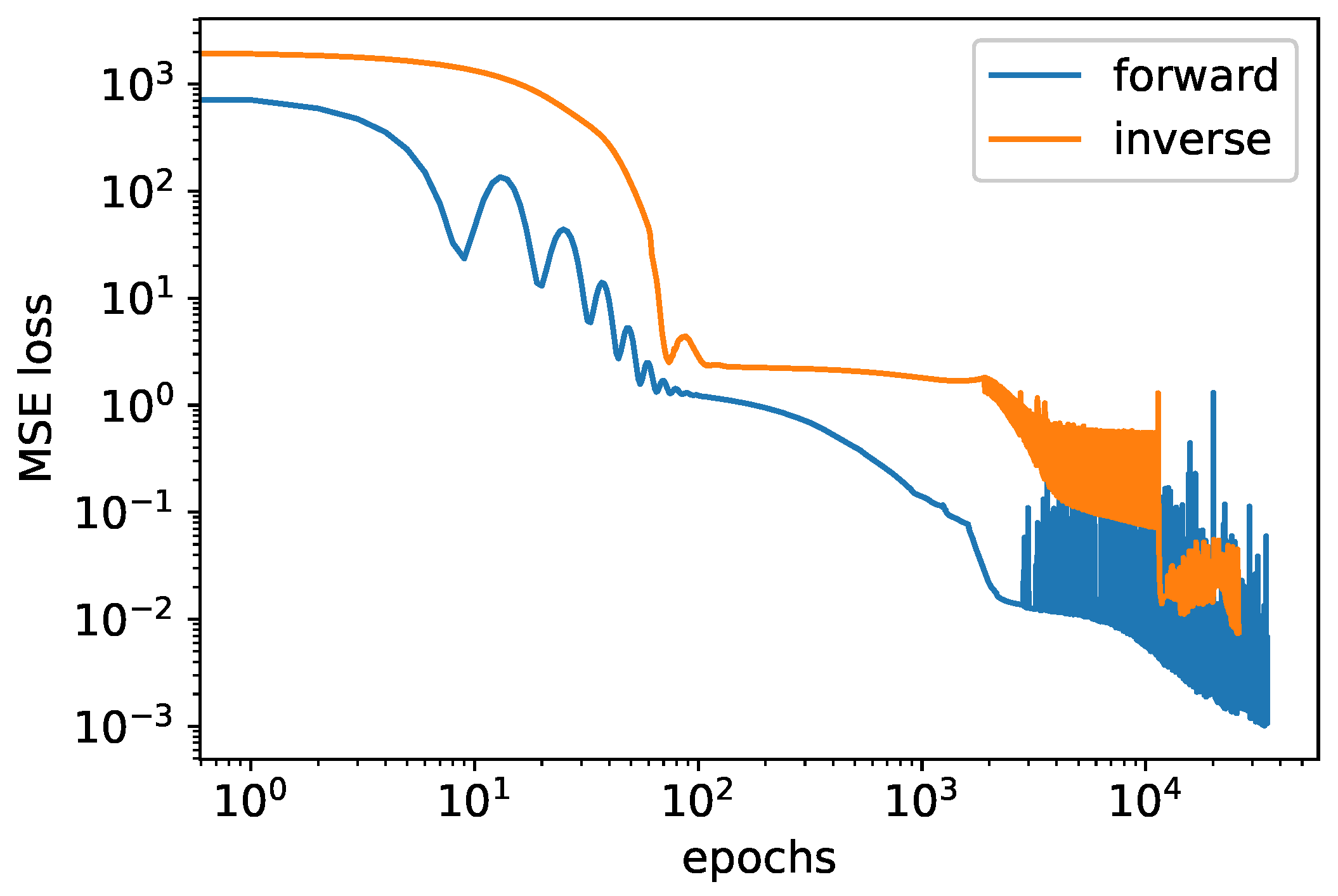
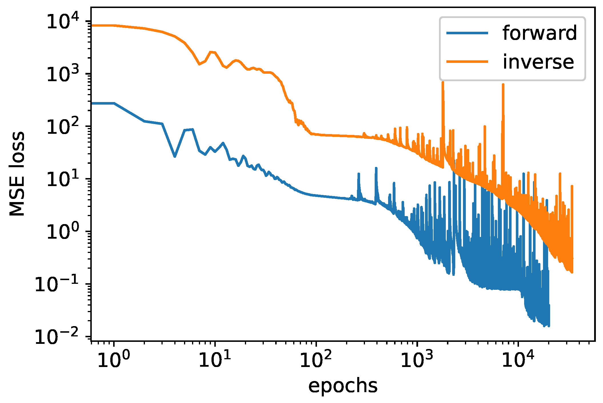
Figure 2a and Figure 3 show the direct problem solution quality using the PINN in the form of a time–pressure profile according to the sample from the initial stage of injection $t=175\mathrm{s}$ (upper line) to the moment of time E = 86,000 s (bottom line) compared with the finite difference approach. Apparently the allocation of the PINN leads to a good solution quality for the direct problem. The rRMSE score corresponds to a 95% confidence interval for a set of 10 algorithms launches. From the series of experiments, it was obtained that the confidence interval is rRMSE = (0.001099, 0.001602) rRMSE = (0.001099, 0.001602). The reduction in loss function values during the training step is demonstrated in Figure A1 (for the forward and inverse tasks).

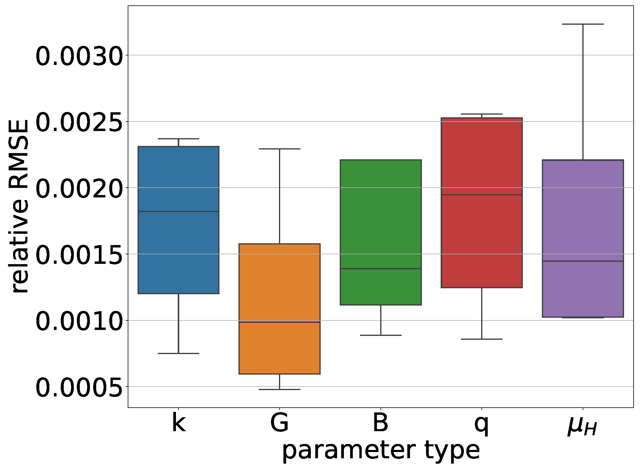
A series of experiments was conducted to investigate the algorithm’s stability to changes in input parameters. Figure 4 illustrates the stability of the solution while the input parameters are changed. Each box represents the variability of one parameter while the others remain constant, as shown in Table 1. A grid of four values has been defined for each parameter, as shown in

Table 2. A table displaying the changes in parameter values for the series of experiments shown in Figure 4.

Parameters	Values
$k,\mathrm{mD}$	$[0.1,0.5,1,5]$
$G,\frac{\mathrm{MPa}}{\mathrm{m}}$	$[0.25,2.5,25,250]\times {10}^{-3}$
$B,\frac{\mathrm{m}}{\mathrm{Pa}}$	$[{10}^{-2},{10}^{-3},{10}^{-4},{10}^{-5}]$
$q,\frac{\mathrm{m}}{\mathrm{day}}$	$[0.02,0.1,0.2,0.3]$
${\mu }_H,\mathrm{mPa}·\mathrm{s}$	$[10,50,100,150]$

. The distribution of error values (relative MSE $\sim {10}^{-5}$) indicates the algorithm’s stability to changes in the parameters responsible for the flow nonlinearity.

The inverse problem solution is the determination of the rheological properties of the fluid based on data obtained from laboratory experiments, where changes in the dynamics of the flow velocity at various pressure gradients were observed [23]. The problem solution results are shown in Figure 2b in the form of velocity dependencies on the pressure gradient modulus in comparison with experimental data, the values of which are reflected on the right scale.

The loss function in the case of the inverse problem solution is identical to expression (11), but contains an additional term ${\lambda }_d\left|\right|{\mathcal{L}}_d{\left|\right|}_2{|}_Z$, where ${\mathcal{L}}_d=w_{data}-w_{pred}$. $w_{pred}$ is the PINN-algorithm-calculated flow velocity, $w_{data}$ is the experimentally measured velocity value, $\mathrm{\Theta }$ are neural network parameters, and Z is the set of dots (experimental data). Further, the optimization problem solution result is a parameterized function (neural network) corresponding to the solution of system (9), (10) and is in agreement with the experimental data. Also, coefficients $G,B,{\mu }_H$ were assessed; they determine the function of viscosity on pressure gradient from which the optimal (according to the optimization algorithm) solution is obtained. The neural network applied to the direct problem solution was applied to the inverse problem solution as well. Adam was also selected as an optimizer with an optimization step of lr = 1 × 10⁴, and the number of optimization steps was epoch = 26,000, ${\lambda }_r=1$, ${\lambda }_b=100$, ${\lambda }_d=10$. The initial guess and final values of the searched parameters are demonstrated in

Table 3. The initial and final values of the desired parameters obtained from solving the inverse problem.

Parameters	Initial Guess	Final Values
$G,\frac{\mathrm{MPa}}{\mathrm{m}}$	$0.09\frac{p_k}{L}$	$0.007\frac{p_k}{L}=0.0187$
$B,\frac{\mathrm{m}}{\mathrm{Pa}}$	$2\times {10}^{-3}$	$0.292\times {10}^{-3}$
${\mu }_H,\mathrm{mPa}·\mathrm{s}$	30	$24.8$

.

Figure 2b also shows the viscosity change function with the determined parameters (numerical viscosity values are displayed on the left scale).

3.2. Field Experiment Interpretation

As a second example, we considered the production task of hydrodynamic data interpretation [7]. In an undisturbed circular reservoir (of thickness H with a given reservoir radius $R_k$, where the pressure is close to the reservoir pressure $P_0$), the well initially has a constant flow rate Q and a depth sensor is located at the bottom hole and records pressure values over time. According to hydrodynamic research, it is necessary to determine the current parameters of the reservoir system (permeability, reservoir porosity, fluid parameters). The mathematical formulation of the problem is represented by system (8), but is written in a cylindrical symmetric formulation and supplemented with boundary conditions for a well of radius $r_0$, taking into account well imperfections, using a given coefficient C [22]:

$$\begin{array}{c}\left\{\begin{array}{c}2\pi Hr\frac{k}{\mu }\frac{\partial p}{\partial r}{|}_{(r=r_0)}=Q+C\frac{\partial p}{\partial t}{|}_{(r=r_0)}\hfill \\ p(R_k,t)=P_0\hfill \\ p(r,0)=P_0\hfill \end{array}\right.\\ (r,t)\in [r_0,R_k]\times [0,T]\subset \mathrm{\Omega }\end{array}$$

(13)

By analogy with the transformation of system (8) to system (9) after non-dimensioning ($\overline{p}=\frac{p}{P_0}$, $\overline{r}=\frac{r}{R_k}$, $\overline{t}=\frac{t}{T}$) a system including nonlinear flow equations, the initial and boundary conditions on the reservoir radius and well bottom are obtained. To create a grid condensing to $r_0$, a transition to logarithmic coordinates $u=ln\overline{r}$ was carried out:

$$\begin{array}{c}\left\{\begin{array}{c}\frac{R_k^2{e}^{2u}{\beta }_{*}}{kT}\frac{\partial \overline{p}}{\partial \overline{t}}-\frac{\partial }{\partial u}\left(\frac{1}{\mu }\frac{\partial \overline{p}}{\partial u}\right)=0,\hfill \\ \mu =\frac{{\mu }_H-{\mu }_L}{1+exp\frac{B{P}_0}{R_k}\left(\right|\frac{1}{e^u}\frac{\partial \overline{p}}{\partial u}|-\frac{R_k}{P_0}G)}+{\mu }_L,\hfill \\ \frac{\partial \overline{p}}{\partial u}{|}_{(u=ln\frac{r_0}{R_k})}=\frac{Q\mu }{2\pi kH{P}_0}+\frac{C\mu }{2\pi kHT}\frac{\partial \overline{p}}{\partial \overline{t}},\hfill \\ \overline{p}(u=ln\overline{r},0)=1,\hfill \\ \overline{p}(u=ln\left(1\right),\overline{t})=1.\hfill \end{array}\right.\\ (u,\overline{t})\in [ln\left(\frac{r_0}{R_k}\right),0]\times [0,1]\subset \overline{\mathrm{\Omega }}\end{array}$$

(14)

To solve the direct problem, the loss function is based on Equation (11) on the space-time grid X. ${\mathcal{L}}_b$ is defined as a vector with components:

$$\left\{\begin{array}{c}{\mathcal{L}}_r=\frac{R_k^2{e}^{2u}{\beta }_{*}}{kT}\frac{\partial \overline{p}}{\partial \overline{t}}-\frac{\partial }{\partial u}\left(\frac{1}{\mu }\frac{\partial \overline{p}}{\partial u}\right)\hfill \\ {\mathcal{L}}_b=\left[\frac{\partial \overline{p}}{\partial u}-\frac{Q\mu }{2\pi kH{P}_0}-\frac{C\mu }{2\pi kHT}\frac{\partial \overline{p}}{\partial \overline{t}},\overline{p}(u,0)-1,\overline{p}(0,\overline{t})-1\right]\hfill \end{array}\right.$$

(15)

A fully connected neural network with four hidden layers of 200 neurons and hyperbolic tangents as an activation function was applied. The weighting coefficient ${\lambda }_r$ was set as a function [25] of ${\mathcal{L}}_r$, ${\lambda }_b=1000$. Adam was used as an optimizer with an optimization step of lr = 1 × 10⁻³, and the number of iterations was epoch = 20,000. $\overline{\mathrm{\Omega }}$ was covered by a discrete rectangular grid $X=(N_x,N_t)$, which consisted of $N_{\overline{t}}=50$ and $N_u=120$ collocation points. The uniform grid along the u direction made it possible to reduce the grid step for the $\overline{r}$ direction in areas of large pressure gradients. The input data used to solve the problem are given in

Table 4. The input parameters to solve the direct problem.

$r_c=0.1\mathrm{m}$	$R_k=100\mathrm{m}$	$H=10\mathrm{m}$
$m=0.134$	$k=50\mathrm{mD}$	${\beta }_{*}={10}^{-10}{\mathrm{Pa}}^{-1}$
${\mu }_L=25\mathrm{mPa}·\mathrm{s}$	${\mu }_H=250\mathrm{mPa}·\mathrm{s}$	$G=0.005\frac{\mathrm{MPa}}{\mathrm{m}}$
$B=2\times {10}^{-3}\frac{\mathrm{m}}{\mathrm{Pa}}$	$p_0=25\mathrm{MPa}$	$Q=7.8\frac{{\mathrm{m}}^3}{\mathrm{day}}$
$T=5\mathrm{days}$	$L=100\mathrm{m}$	$C=0.0671{\mathrm{MPa}}^{-1}$

.

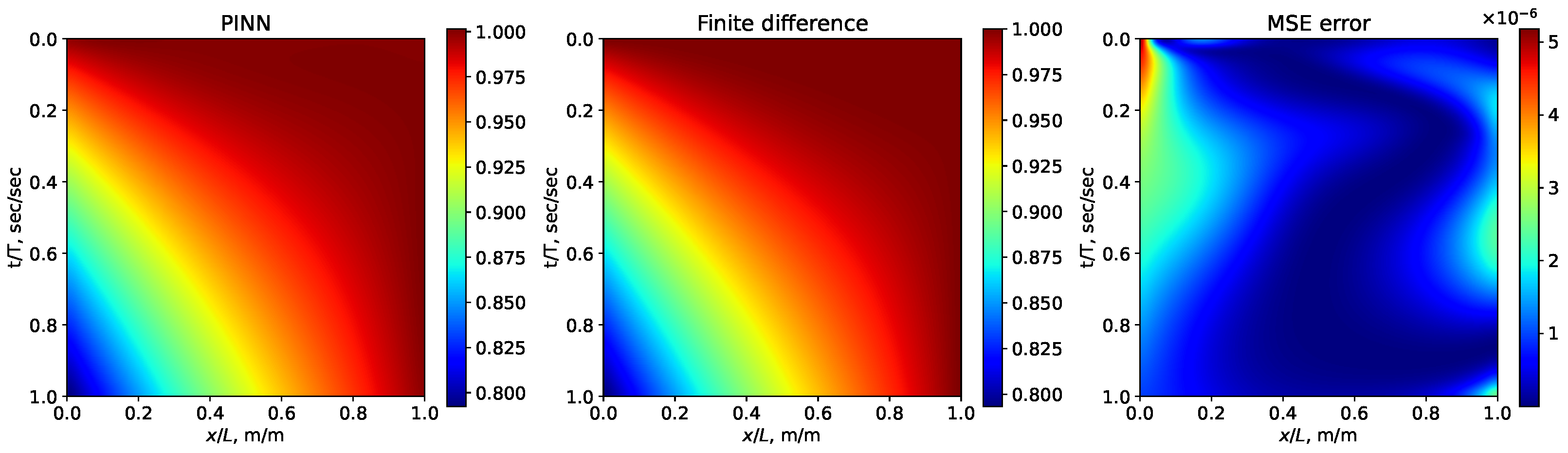
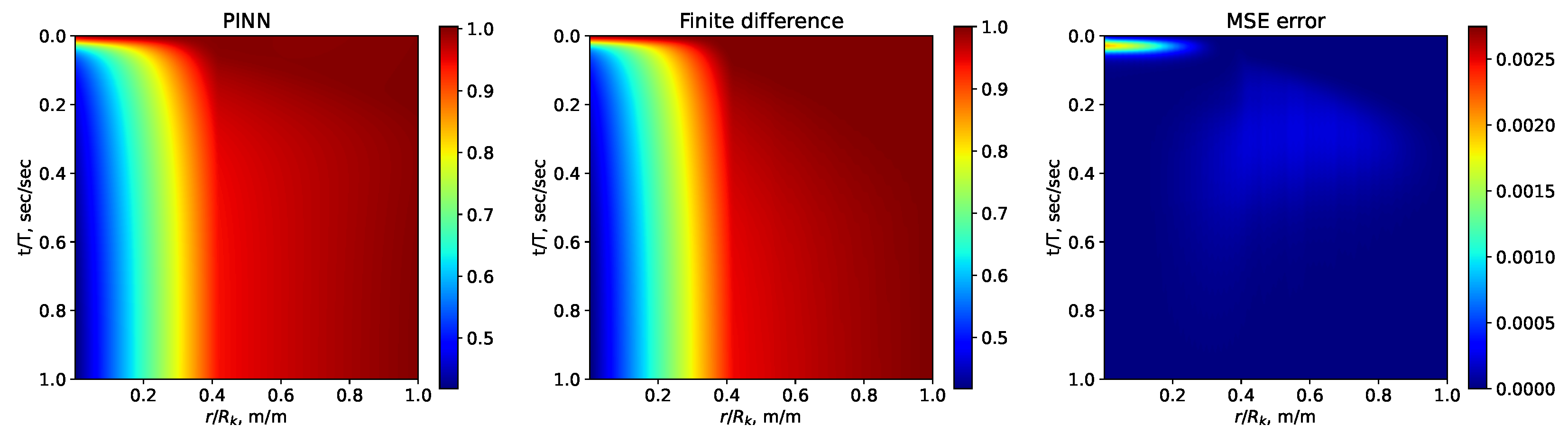
Figure 5 and Figure 6 show a comparison of the reservoir pressure distributions calculated by the PINN and finite difference approaches. Figure 5 shows a comparison of reservoir pressure distributions (a) and well pressure drops (b) at various points in time calculated by the PINN (pinned points) and the finite difference (dotted lines) approaches. The rRMSE estimation was performed as a 95% confidence interval for a set of 10 algorithm launches. From the experiments series, it was found that the confidence interval rRMSE = (0.00687, 0.00779). The reduction in loss function values during the train step is demonstrated in Figure A2 (for the forward and inverse tasks).

The pressure values obtained by the sensors at the well’s bottom hole were used as experimental data for solving the inverse problem (determining reservoir parameters based on log results). The loss function in the case of the inverse problem solution is identical to Equation (11) with an additional term ${\lambda }_d\left|\right|{\mathcal{L}}_d{\left|\right|}_2{|}_Z,{\mathcal{L}}_d=p_{data}-p_{pred}$. Here, $p_{pred}$ is the calculated pressure values at the bottom hole, $p_{data}$ is experimentally measured downhole pressure value, $\mathrm{\Theta }$ are neural network parameters and Z is the set of dots where experimental data were changed. The numerical solution of the equation system (14) was obtained, and the vector of coefficients $G,C,k,{\mu }_H$ is defined as the inverse problem solution results. For the inverse problem, a fully connected neural network with nine hidden layers of 100 neurons was applied, and a hyperbolic tangent was used as the activation function. Adam was chosen as the optimizer with the optimization step of lr = 1 × 10⁻³, and the number of optimization steps was epoch = 24,000. ${\lambda }_r=1$, ${\lambda }_b={10}^4$ and ${\lambda }_d={10}^4$. The initial guess and final values of the searched parameters are demonstrated in

Table 5. The initial and final values of the desired parameters obtained from solving the inverse problem.

Parameters	Initial Guess	Final Values
$C,\frac{{\mathrm{m}}^3}{\mathrm{MPa}}$	1	$1.8768$
$G,\frac{\mathrm{MPa}}{\mathrm{m}}$	$0.02$	$0.013$
${\mu }_H,\mathrm{mPa}\mathrm{s}$	25	38

.

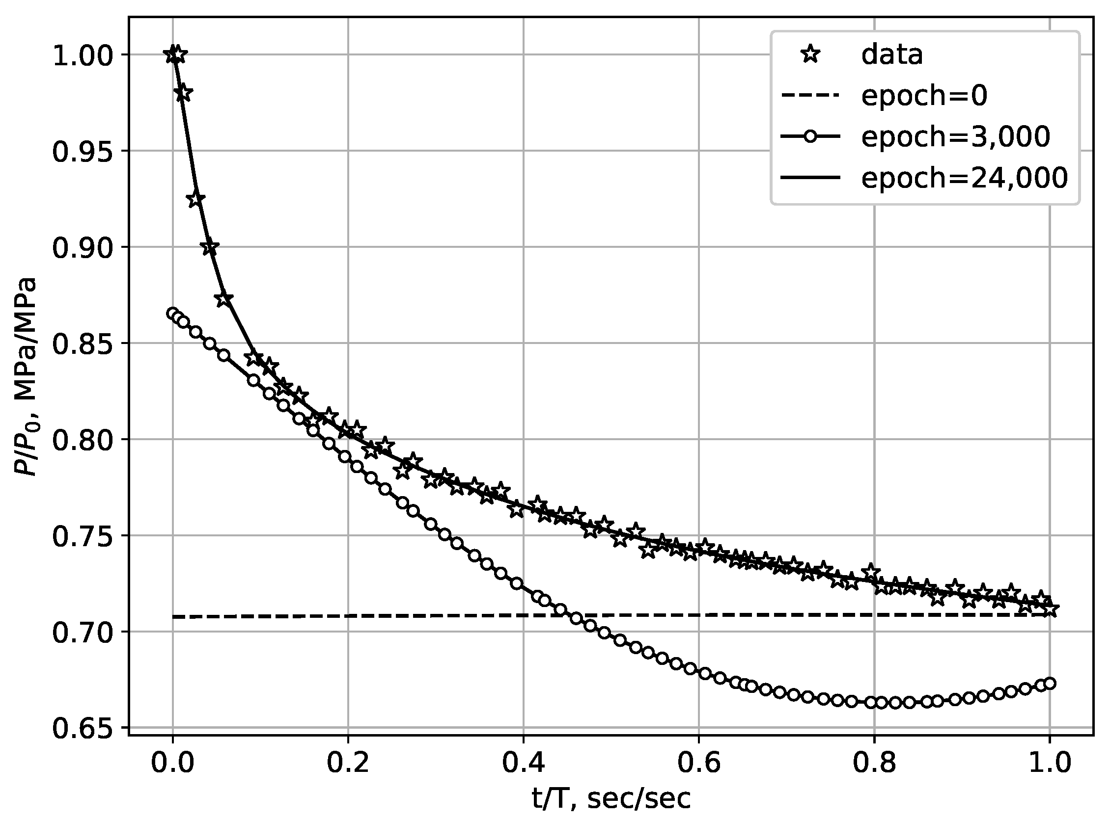
Figure 7 shows that the inverse problem solution results in pressure changes at the bottom hole at various optimizer steps in comparison with the experimental data (marked with circles). The initial guess is indicated at Figure 7 as a horizontal dotted line (epoch = 0).

4. Discussion

Considering the problems of increasing oil recovery, it is necessary to take into account a whole range of phenomena that affect the displacement characteristics and appear during the application of complex thermo-chemical methods to saturated reservoirs. Among these are the heterogeneity, as the initial distribution of the filtration-capacitance properties of the layers (porosity, permeability, pore distribution by size), as well as these properties’ changes over time, which occur mainly due to the pumped active agents’ interactions with both the formation liquid and the porous skeleton (phase transitions, chemical reactions, sorption/desorption processes) [3,26]. In addition, the unsteadiness of the development processes in combination with changes in the fluid properties’ dynamics leads to the necessity to modify the flow additive components (responsible for mass transfer and energy inflow) in the conservation equations (mass, momentum, energy) which describe the process, and also to modify the equation type, which leads to the necessity of changing the calculation algorithm while modeling.

In this paper, considering the change in the reservoir fluid’s rheology during a non-stationary process, which is expressed as a change in the equation of motion due to a decrease in fluid viscosity with a pressure gradient increase (due to structural failure), the solution of the filtration problem using the parameterized PINN function is shown. Based on the generalization of the latest/newest experiences of using PINNs in various tasks, the authors of this paper have formulated a deviation/error function that accounts for the physical conservation equations and initial and boundary conditions based on the data from laboratory and/or field experiments. The sensitivity of the parameterized model to changes in the set of input parameters is analyzed.

Pseudoplastic liquid flow simulations applying a PINN in the processing of laboratory experiments on real core samples in comparison with “classical” solving methods [1], a similar “nonlinear” problem for PDEs, showed that PINN algorithms allowed for the obtention of a stable solution to both the direct and inverse problems of pseudoplastic filtration theory with lower resource costs.

Thus, the numerical studies carried out confirm the possibility of describing the specifics of an unsteady filtration process of non-Newtonian liquids in a porous medium with changing properties via the PINN approach. The results of laboratory experiments on core processing and the data from hydrodynamic studies of a real field were considered, and it was established that the convergence of the results obtained via the PINN and the results obtained using finite difference methods is good, with an rRMSE metric on the order of 1 × 10⁻³.

It should also be noted that PINNs are universally applicable when changing both the form of the equations and the type of initial boundary conditions. This makes it possible to unify algorithms of filtration theory for direct and inverse solution investigations, in contrast to finite-difference methods, where specification of the algorithm for each type of PDE system is required. The results of the inverse problem solution showed that the algorithm applied is stable to the choice of the initial approximation (for some parameters, the initial conditions were different by orders of magnitude), which reduces the role of the expert in the solution search process and improves the stability of the solution.

In the proposed formulation of the problem, the task of selecting hyperparameters (coefficient of regularization, choice of optimizers, step of gradient descent, etc.) remains relevant, which is typical for optimization problems. However, in recent studies, where algorithms for adaptive parameter selection are proposed [27], it was shown that the application of parameterized models with a PINN is highly efficient and can potentially produce descriptions of the complex filtration processes of pseudoplastic liquids at the proper level.

5. Conclusions

Based on the physical laws of non-Newtonian liquid flows in a porous medium and considering the initial and boundary conditions and data from physical experiments, a deviation function is formulated which is minimized during the search for solutions of filtration problems via a PINN. The analysis of the proposed parameterized model revealed a lack of sensitivity to changes in the set of input parameters. Validation of the model under study, carried out on the data from one-dimensional physical experiments, showed the convergence of the calculated and experimental data. Based on the results obtained, further development of the model in two-dimensional and three-dimensional formulations is possible.