Semi-Online Algorithms for the Hierarchical Extensible Bin-Packing Problem and Early Work Problem

Abstract

In this paper, we consider two types of semi-online problems with hierarchies. In the extensible bin-packing problem with two hierarchical bins, one bin can pack all items, while the other bin can only pack some items. The initial size of the bin can be expanded, and the goal is to minimize the total size of the two bins. When the largest item size is given in advance, we provide some lower bounds and propose online algorithms. When the total item size is given in advance, we provide some lower bounds and propose online algorithms. In addition, we also consider the relevant early-work-maximization problem on two hierarchical machines; one machine can process any job, while the other machine can only process some jobs. Each job shares a common due date, and the goal is to maximize the total early work. When the largest job size is known, we provide some lower bounds and propose two online algorithms whose competitive ratios are close to the lower bounds.

1. Introduction

The bin-packing problem (BP) is one of the most fundamental problems in combinatorial optimization and is the cornerstone of approximation algorithms, and it has been extensively studied since the early 1970s. The extensive study of the BP, called the extensive bin-packing problem (EBP), has had a great impact on the design and analysis of approximation algorithms [1,2], which are widely used in numerous classic applications, such as machine scheduling, cutting stock problems, storage allocation, and cloud storage. Currently, the model of the EBP arises in scheduling problems [3], and more and more hierarchical scheduling has been combined with early work maximization (especially makespan minimization) in recent years [4] (especially [5,6,7]). Thus, in this work, we will investigate both problems: the hierarchical extensible bin-packing problem and the early-work-maximization problem. Before introducing our problems, we will first provide some basic knowledge and related notions, the contributions of previous studies, and the motivation and the results of this paper.

1.1. Basic Knowledge and Related Notions

In the (semi-)online scheduling problem, the jobs arrive one by one. The performance of the (semi-)online algorithm is measured by the competitive ratio. For a maximization (minimization) problem and given an instance I, the objective value of the solution produced by an online algorithm A is denoted by $C^A\left(I\right)$ ($C^A$, for short), and the offline optimal criterion value is denoted by $C^{\ast }\left(I\right)$ ($C^{\ast }$, for short). The performance of A is measured by its competitive ratio, and the competitive ratio of A is defined as the minimum value $\rho$ satisfying $C^{\ast }\left(I\right)\le \rho ·C^A\left(I\right)$ ($C^A\left(I\right)\le \rho ·C^{\ast }\left(I\right)$) for any instance I, where $C^A\left(I\right)$ denotes the output value by A and $C^{\ast }\left(I\right)$ denotes the offline optimal criterion value. On the other hand, if there is no online algorithm for the problem that has a competitive ratio strictly less than $\gamma$, then $\gamma$ is referred to as a lower bound of the problem. In particular, if there is an online algorithm with a competitive ratio exactly matching the problem’s lower bound, then we claim that this algorithm is an optimal online algorithm.

For the online hierarchical extensible bin-packing problem, we are given a set $I=\{a_1,a_2,\dots ,a_n\}$ of n items. Each item $a_j$ has a size $s_j$ and m extendable bins $B_1,B_2,\dots ,B_m$ with original size 1, where each item must be packed into one bin, and the total size of the items packed in any bin can exceed 1, if necessary. The load $L_i={\sum }_{j:a_j\in B_i}{s}_j$ of a bin $B_i$ is just the total size of the items contained in $B_i$, and the size of a bin $B_i$ is defined by $max\{L_i,1\}$. The extensible bin-packing problem introduced in [3,8], which is also called operating room allocation [9], is to minimize the total size of the bins, i.e., to minimize

$$S=\sum _{i=1}^m{s}_i=\sum _{i=1}^{m}max\{L_i,1\}.$$

Since the model of the EBP naturally arises in scheduling problems, we stick to the scheduling terminology in this article (bins are the same as machines; items are the same as jobs). For the semi-online hierarchical early work maximization scheduling problem, we are given a set $\mathcal{M}=\{M_1,M_2\}$ of two hierarchical machines and a set $\mathcal{J}=\{J_1,J_2,\cdots ,J_n\}$ of n jobs arriving online. The machine $M_1$ can process all jobs, while the machine $M_2$ can only process some of the jobs. Each job can only be processed by one machine. A new job $J_{j+1}$ arrives only after job $J_j$ is irrevocably scheduled to a machine. Let $L_i={\sum }_{J_j\in S_i}{p}_j$ be the load of $M_i$, $i\in \{1,2\}$. The objective is to find a schedule such that the total early work

$$X=\sum _{j=1}^n{X}_j=\sum _{i=1}^{2}min\{L_i,1\}$$

is maximized.

1.2. The Contributions of Previous Studies

The extensible bin-packing problem (EBP), with the goal of minimizing the total sizes of bins, originates from the research work of Dell’Olmo et al. [8], who showed that the problem is strongly NP-hard. Furthermore, they proved that the approximation ratio of the longest processing time (LPT) algorithm for the problem is $\frac{13}{12}$.

Alon et al. [10] presented a unified efficient polynomial time approximation scheme (EPTAS) for scheduling on parallel machines, which is also suitable for the EBP. It is worth noting that Coffman et al. [11] presented an asymptotic fully polynomial time approximation scheme (FPTAS) for the EBP. If the number m of bins is fixed, there is an FPTAS following from the results of [12]. Most recently, Levin [13] designed an EPTAS for a generalization of the EBP with unequal bin sizes, where the cost of exceeding the bin size depends on the index of the bin and not only on the amount by which the size of the bin is exceeded.

A special case of the EBP is the case of extensible bin packing with unequal bin sizes (called the EBP-UBS). The online version of the problem was first studied by Dell’Olmo et al. [14], and they proved that the competitive ratio of the LS algorithm is $\frac{5}{4}$, which was improved slightly by Ye et al. [15]. Berg et al. [16] gave an online algorithm for the online EBP with a variable cost of extension. Most recently, Luo et al. [17] presented several lower bounds and an online algorithm whose competitive ratio is optimal in certain cases for the online EBP with a variable cost of extension. When $m\ge 3$, there exists a big gap between the best-known lower bound and the upper bound for the online EBP. When $m=2$, the best possible competitive ratio for the online EBP problem is $\frac{7}{6}$ [3,18]. Another special case of the EBP is the case of a stochastic extensible bin-packing problem (SEBP), in which the size of each item follows some known probability distribution, and all the n items are packed into m bins of unit capacity in order to minimize the expected costs. Sagnol et al. [19] showed that there is a simple policy, called LEPT, with an approximation ratio of $1+e^{-1}\approx 1.368$ for the SEBP, and the problem has been generalized to arbitrary stochastic jobs in [20]. Building on the two papers, Sagnol et al. [21] proved improved bounds under distributional assumptions of the processing times.

The EBP model arises in scheduling problems in which machines are available for some amount of time at a fixed cost and for extra time at an additional cost. Speranza et al. [3] first introduced the online scheduling problem on m identical machines with extendable working time, which is also a special online EBP problem in which all bin sizes are equal to one and the size of a bin can be extended if necessary. They proved that the competitive ratio of the list scheduling (LS) algorithm for the problem is $\frac{5}{4}$ and designed a new online algorithm with a competitive ratio of $1.228$.

A similar problem is the early work maximization scheduling problem. Nonpreemptive parallel machine scheduling with a common due date to maximize the total early work of all the jobs, i.e., the total processing time of the jobs completed before the common due date, has been a popular objective in the past decade [22,23]. Recently, for the offline version of the problem, when the number m of machines is fixed, Li [24] presented an FPTAS with running time $O(\frac{1}{{ϵ}^{2m+1}}+n)$, for any desired accuracy $ϵ$, where n is the number of jobs and $f\left(\frac{1}{ϵ}\right)$ is exponential in $\frac{1}{ϵ}$. When the number m of machines is not fixed, Li [24] also presented an EPTAS. Moreover, Sun et al. [25] proved that the worst-case ratio of the LPT algorithm for the offline early-work-maximization problem is at most $1.207$ this year. For the online case of the problem, Chen et al. [26] considered the scheduling problem on parallel identical machines and presented an algorithm with a competitive ratio of $\frac{\sqrt{2m^2-2m+1}-1}{m-1}$. In particular, they proved that the competitive ratio of $\sqrt{5}-1$ is tight when $m=2$. This year, Jiang et al. [27] proved that the tight competitive ratio of the LS algorithm is $\frac{4}{3}$ and improved the upper bound on the competitive ratio for the previous algorithm $EF{F}_m$ to $1.2956$.

For the early-work-maximization problems on two hierarchical machines, Xiao et al. [28] studied two semi-online models of the problem with a buffer or rearrangements. If a buffer size of K is available, they designed an optimal online algorithm with a competitive ratio of $4/3$. If it is allowed to reassign at most K jobs after all the jobs have been scheduled, they proposed an optimal online algorithm with a competitive ratio of $4/3$. Furthermore, Xiao et al. [7] designed an optimal online algorithm with a competitive ratio of $\sqrt{2}$ for the problem and proposed several optimal semi-online algorithms for the cases when the largest processing time or total processing time is known. For the early-work-maximization problems on two hierarchical uniform machines $M_1$ and $M_2$, where machine $M_1$ with speed $s>0$ is available for all jobs and machine $M_2$ with speed 1 is available only for high-hierarchy jobs, Xiao et al. [4] proposed four optimal semi-online algorithms for the cases of the total size of all jobs, the total size of low-hierarchy jobs, the total size of high-hierarchy jobs, and both the total size of low-hierarchy and high-hierarchy jobs that are known in advance, respectively. This problem is also closely related to the online $l_p$-norm load-balancing problem on two hierarchical machines [6,29] and the online machine covering problems on two hierarchical machines [30,31,32]. Furthermore, more related results can be found in the recent surveys [33,34,35].

The makespan minimization scheduling problem on hierarchical machines is another typical objective in scheduling and is also closely related to the online early-work-maximization problem. The online version of such a problem was also first studied by Park et al. [36] and Jiang et al. [37]. They independently proposed an optimal online algorithm with a competitive ratio of $\frac{5}{3}$. Moreover, if the total size of all the jobs is given in advance, ref. [36] presented an optimal online algorithm with a competitive ratio of $\frac{3}{2}$. If the largest processing time of jobs is known in advance, Wu et al. [38] presented an optimal online algorithm with a competitive ratio of $\frac{1+\sqrt{5}}{2}$; if the total processing time is known in advance, the group presented an optimal online algorithm and obtained the same result as [36]. If the processing times are bounded, Liu et al. [39], Luo et al. [40], and Zhang et al. [41] designed several online algorithms for the makespan minimization problem on two hierarchical machines. Chen et al. [22,42] considered several semi-online versions of the problem and proposed the corresponding optimal online algorithms. Akaria et al. [5] discussed online scheduling with migration on two hierarchical machines.

1.3. The Motivation of the Paper

The EBP has been widely used to represent the cost of allocating surgeries to operating rooms (ORs) [9,16,19] in recent years, which is a challenging combinatorial optimization problem. There is also significant uncertainty in the duration of surgical procedures, which further complicates assignment decisions. In the context of OR allocation, ORs represent bins. Assume that $k\le m$ is the number of ORs. Each bin has a certain size at a fixed cost $c^f$, which denotes the time T that each OR is available during a particular day. The OR can be utilized for more than the regular available time. Under this model, the total cost of a solution assigning the subset of surgeries $S_i$ to the i-th operating room ($i=1,\cdots ,k$) becomes $k{c}^f+c^v{\sum }_{i=1}^{k}max\{{\sum }_{j\in S_i}{p}_j-T,0\}$, and the decision maker is asked to find the best allocation so that the total cost is minimized. The EBP corresponds to the situation in which $T=c^f=c^v=1$ and $k=m$. In practice, surgical durations are not known in advance, and the patients with more severe injuries should be given priority treatment, which is also highly important. In addition, in communications engineering, service providers assign service classes to calls in communications networks and route queries to hierarchical databases. Hence, motivated by these random cases and online hierarchical scheduling [43], we study the hierarchical extensible bin-packing problem (HEBP), in which each bin $B_i$ has an identical original size 1, for $i=1,2$. The bin $B_1$ can pack all the items, while $B_2$ can only pack the items with the high hierarchy, i.e., $h_j=2$, with the objective of minimizing the expected costs. Our new model is defined to generalize some special semi-online cases of the HEBP.

Scheduling with the goal of early work maximization has many practical applications in recent years, such as scheduling customer orders in manufacturing systems, testing software in software engineering, spreading fertilizers in agriculture, planning technological processes in manufacturing systems, collecting data from sensors in control systems, and harvesting crops in agriculture. For example, in the service industry, service providers often assign corresponding privileges and differentiated services to customers according to the level of service they promise to customers. Motivated by [32], we study the early-work-maximization problems on two identical parallel machines under a grade of service (GoS) provision, with the information of the largest job, where the machine $M_1$ can process all jobs, while the machine $M_2$ can only process the higher hierarchical jobs, with the goal of maximizing the total early work. Our new model is defined to generalize some special semi-online cases of the problem.

1.4. The Organization and Results of the Paper

The remainder of this paper is organized as follows.  Section 2 focuses on a series of models for the HEBP with the largest item size known in advance.

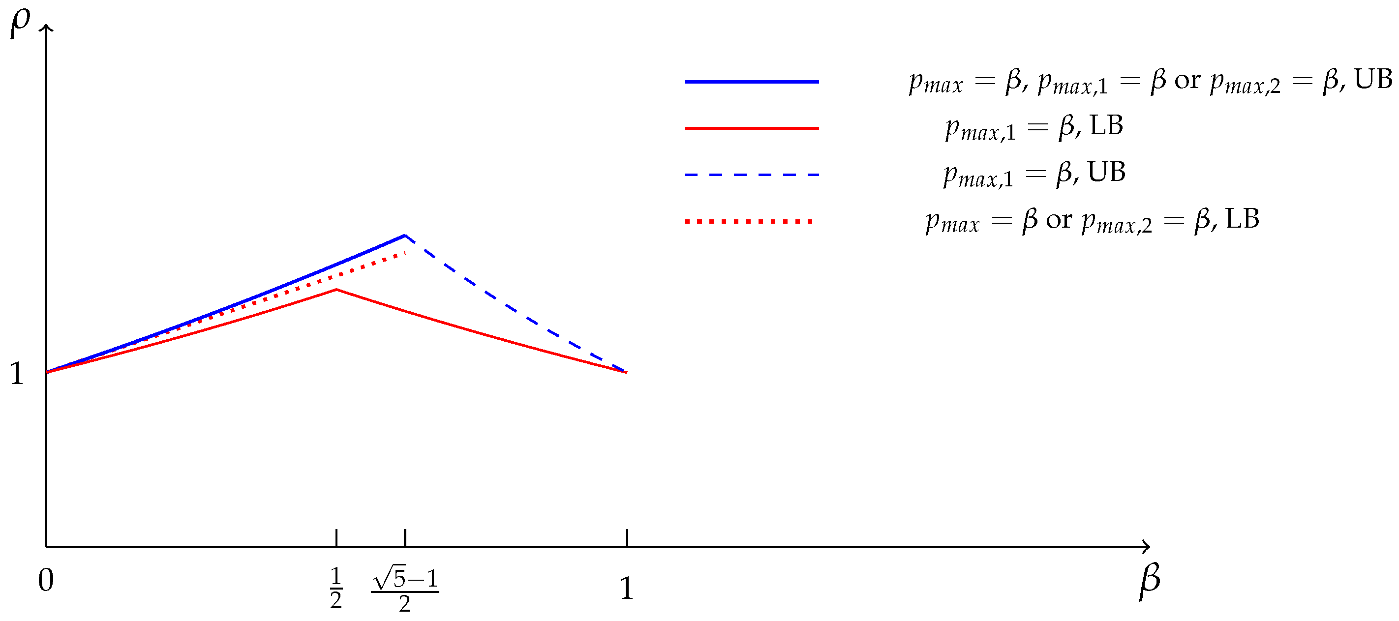
(Section 2.1) If the largest size $\beta$ of the items is known in advance, without knowledge of the item hierarchy, and if at least one item of size $\beta$ appears, we give two lower bounds $1+\frac{\beta }{4}$ and $1+\frac{1}{2+2\beta }$ and propose an optimal online algorithm with a competitive ratio of $1+min\{\frac{\beta }{4},\frac{1}{2+2\beta }\}$.

(Section 2.2) If the hierarchy of the largest item is known in advance and there is at least one item of the largest size $\beta$ that appears, we give some lower bounds. When $\frac{2}{3}<\beta <1$, we propose a simple online algorithm with a competitive ratio of $\frac{3-\beta }{2}$.

(Section 2.3) If the largest item with hierarchy $h_j=1$ is known in advance and if $\beta =1$, i.e., $s_j\le s_{max,1}\le 1$, where $s_{max,1}$ is the size of the largest item $a_{max,1}$ with the lower hierarchy, we design an optimal semi-online algorithm with a competitive ratio of $\frac{7}{6}$.

(Section 2.4) If the largest item with hierarchy $h_j=2$ is known in advance and considering the case where $\beta =1$, i.e., $s_j\le s_{max,2}\le 1$, where $s_{max,2}$ is the size of the largest item $a_{max,2}$ with the higher hierarchy, we show a lower bound $\frac{\sqrt{13}+1}{4}$ and design an online algorithm with a competitive ratio of $\frac{7}{6}$.

Section 3 focuses on a series of models for the HEBP with the total item size known in advance.

(Section 3.1) If the total size T of all the items is known in advance, we give a lower bound of $\frac{5}{4}$ and propose an optimal online algorithm with a competitive ratio of $\frac{5}{4}$.

(Section 3.2) If the total size $T_1$ of the low-hierarchy items is known in advance, we show a lower bound of $\frac{\sqrt{13}+1}{4}$ and propose an algorithm with a competitive ratio of $\frac{7}{6}$.

(Section 3.3) If the total size $T_2$ of the high-hierarchy items is known in advance, we show a lower bound of $\frac{\sqrt{13}+1}{4}$ and propose an algorithm with a competitive ratio of $\frac{7}{6}$.

In Section 4, we investigate the semi-online hierarchical early-work-maximization problem, i.e., the case of the largest job is known in advance.

(Section 4.1) If the largest job size $p_{max}=\beta \le 1$ is known in advance, without knowledge of the job hierarchy, we give two lower bounds $1+\frac{\beta }{3}$ and $\frac{\sqrt{{\beta }^2-2\beta +9}-1+\beta }{2}$ for $\beta <\frac{\sqrt{5}-1}{2}$ and $\frac{\sqrt{5}-1}{2}\le \beta \le 1$, respectively. We also propose an online algorithm with a competitive ratio $\frac{\sqrt{{\beta }^2-2\beta +9}-1+\beta }{2}$ for $0<\beta \le 1$.

(Section 4.2) If the hierarchy of the largest job is known, when the largest job has a low hierarchy, i.e., $p_j\le p_{max,1}=\beta \le 1, \mathrm{for} 1\le j\le n$, we denote this problem as $P2|GoS,online,p_{max,1}=\beta |max\left(X\right)$. We give two lower bounds $\frac{4}{4-\beta }$ and $\frac{4}{3+\beta }$ for $\beta \le \frac{1}{2}$ and $\frac{1}{2}<\beta \le 1$, respectively.

Finally, we present our conclusions in Section 5.

2. The Hierarchical Extensible Bin-Packing Problem of Knowing the Largest Item Size

For the online case, a set of n items $I=\{a_1,\cdots ,a_n\}$ and two hierarchical bins $B=\{B_1,B_2\}$ are given. Each item $a_j$ is characterized by two parameters: the item size $s_j$ and the item hierarchy $h_j\in \{1,2\}$. For convenience, item $a_j$ is denoted by $a_j=(s_j,h_j)$ for $j=1,\cdots ,n$. Each bin $B_i$ has an identical original size of 1 for $i=1,2$. The hierarchical constraint means that the bin $B_1$ can pack all the items, while $B_2$ can only pack the items with hierarchy 2, i.e., $h_j=2$.

All the items of I are ordered in a list and arrive one by one. Once an item arrives, it must be assigned to one of the two hierarchical bins immediately and irrevocably. The information of item $a_{j+1}$ is given after item $a_j$ has been assigned. Assume that the size of each item satisfies

$$s_j\le 1,\mathrm{for}j=1,\cdots ,n.$$

(1)

This problem is to find a packing that assigns all the items of I to the two bins, and the goal is to minimize the total size of both bins. Let $L_i={\sum }_{a_jϵB_i}{s}_j$ be the load of the bin $B_i$, i.e., the total size of the items assigned to $B_i$, for $i=1,2$. If $L_i\le 1$, the size of bin $B_i$ is equal to 1, i.e., $s_i=1$. If $L_i>1$, the size of bin $B_i$ is equal to its load, i.e., $s_i=L_i$. As a result, the size of bin $B_i$ is defined as

$$s_i=max\{L_i,1\}.$$

Therefore, the goal of the problem is to find a packing plan such that the total size of both bins

$$S=\sum _{i=1}^2{s}_i=\sum _{i=1}^{2}max\{L_i,1\}$$

(2)

is minimized.

In the following, let $L_i^j$ be the total size of the items assigned to bin $B_i$ after item $a_j$ is assigned, for $j\in \{1,2,\cdots ,n\}$. Clearly, we have

$$L_i^n=L_i.$$

Let T be the total size of all the items and $T_k$$(k=1,2)$ be the total size of the items with hierarchy $h_j=k$. Hence, we have $T=T_1+T_2$. Define $C^{\ast }$ as the offline optimal value and $C^A$ as the output value of the (semi-)online algorithm A. From the definition of the total size of both bins, we have the following lemma.

Lemma 1.

The offline optimal value $C^{\ast }$ satisfies

$$C^{\ast }\ge max\{T,2\}.$$

(3)

In this section, we consider a series of models for which the largest item size is given in advance. Assume that each item size $s_j$ is bounded by $(0,\beta ]$, i.e.,

$$0<s_j\le \beta .$$

2.1. The Largest Item Is Known

In this subsection, the largest size of the items is known in advance without knowledge of the item hierarchy, and at least one item of size $\beta$ appears. We give two lower bounds $1+\frac{\beta }{4}$ and $1+\frac{1}{2+2\beta }$ and propose an optimal online algorithm with a competitive ratio $1+min\{\frac{\beta }{4},\frac{1}{2+2\beta }\}$.

Theorem 1.

When only the size of the largest item is known, any online algorithm A has a competitive ratio at least $1+\frac{\beta }{4}$ for $\beta <1$.

Proof. 

Let N be a large enough integer and $\epsilon =\frac{1}{N}$. The first t items are $a_1=a_2=\cdots =a_t=(\epsilon ,2)$, where t is the minimal integer satisfying the following conditions.

Case 1. $L_1^t\in [\frac{\beta }{2},\frac{\beta }{2}+\epsilon ]$ ($L_2^t<1-\frac{\beta }{2}$).

The item $a_{t+1}=(\beta ,1)$ and the last k items $a_{t+2},\cdots ,a_{t+1+k}$ arrive, ${\sum }_{j=t+2}^{t+1+k}{s}_j=1-\beta$ and $s_j\le \beta$, then $C^{\ast }\le 2+\epsilon$ and $C^A\ge 2+\frac{\beta }{2}$.

Case 2. $L_2^t\in [1-\frac{\beta }{2},1-\frac{\beta }{2}+\epsilon ]$ ($L_1^t<\frac{\beta }{2}$).

The last two items $a_{t+1}=(1-\frac{\beta }{2}-L_1^t,1)$ and $a_{t+2}=(\beta ,2)$ arrive, implying that $C^{\ast }\le 2+\epsilon$ and $C^A\ge 2+\frac{\beta }{2}$.

As a result, in all cases, we obtain that

$$\underset{\epsilon \to 0}{lim}\frac{C^A}{C^{\ast }}\ge \underset{\epsilon \to 0}{lim}\frac{2+\frac{\beta }{2}}{2+\epsilon }\ge 1+\frac{\beta }{4}.$$

Therefore, our theorem holds in any case. □

Theorem 2.

When only the size of the largest item is known, any online algorithm A has a competitive ratio of at least $1+\frac{1}{2+2\beta }$ for $\beta \ge 1$.

Proof. 

The first item is $a_1=(\frac{1}{2},2)$.

Case 1. $a_1$ is assigned to $B_1$.

Then, the last item $a_2=(\beta ,1)$ arrives, and we have $C^{\ast }=1+\beta$ and $C^A=\frac{3}{2}+\beta$.

Case 2. $a_1$ is assigned to $B_2$.

Then, the next item $a_2=(\beta ,2)$:

(i)

If $a_2$ is assigned to $B_2$, and no more items arrive, then, we have $C^{\ast }=1+\beta$ and $C^A=\frac{3}{2}+\beta$.

(ii)

If $a_2$ is assigned to $B_1$, the last item $a_3=(\frac{1}{2},1)$ arrives, then we have $C^{\ast }=1+\beta$ and $C^A=\frac{3}{2}+\beta$.

As a result, in all cases, we obtain that

$$\frac{C^A}{C^{\ast }}\ge \frac{\frac{3}{2}+\beta }{1+\beta }=1+\frac{1}{2+2\beta }.$$

Therefore, our theorem holds in any case.    □

The details of our online algorithm are described in Algorithm 1.  

Theorem 3.

The competitive ratio of Algorithm 1 is at most $1+min\{\frac{\beta }{4},\frac{1}{2+2\beta }\}$.

Algorithm 1: A1.

Proof. 

Since the largest item size is $\beta$, we have $C^{\ast }\ge 1+\beta$. Based on Lemma 1, we have $C^{\ast }\ge max\{T,2\}$. In the case of $min\{L_1,L_2\}\ge 1$, we have $C^{A1}=T\le C^{\ast }$. In the case of $max\{L_1,L_2\}\le 1$, we have $C^{A1}=2\le C^{\ast }$. Both cases imply that Algorithm 1 reaches optimality. Thus, we only consider the case of $min\{L_1,L_2\}<1<max\{L_1,L_2\}$, implying that

$$C^{A1}=1+max\{L_1,L_2\}.$$

We consider the following two cases:

Case 1. $L_1>1$ and $L_2<1$.

Let $a_l=(p_l,2)$ be the last item of hierarchy $h_j=2$ assigned to $B_1$. According to Algorithm 1, we know that item $a_l$ is assigned to $B_1$ at Line 9; then, we have

$$L_2\ge L_2^{l-1}\ge max\{1-\frac{\beta }{2},\frac{1}{2}\}.$$

(4)

By Lemma 1, we have

$$\begin{array}{cc}\hfill \frac{C^{A1}}{C^{\ast }}& \le \frac{L_1+1}{max\{2,L_1+L_2,1+\beta \}}=1+\frac{L_1+1-max\{2,L_1+L_2,1+\beta \}}{max\{2,L_1+L_2,1+\beta \}}\hfill \\ \hfill & \le 1+\frac{1-L_2}{max\{2,L_1+L_2,1+\beta \}}\le 1+\frac{1-L_2}{max\{2,1+\beta \}}\hfill \\ \hfill & \le 1+\frac{min\{\frac{\beta }{2},\frac{1}{2}\}}{max\{2,1+\beta \}}=1+min\{\frac{\beta }{4},\frac{1}{2+2\beta }\},\hfill \end{array}$$

where the second inequality follows from $max\{2,L_1+L_2,1+\beta \}\ge L_1+L_2$, the third inequality follows from $max\{2,L_1+L_2,1+\beta \}\ge max\{2,1+\beta \}$, and the last inequality follows from (4).

Case 2. $L_1<1$ and $L_2>1$.

Let $a_t=(s_t,2)$ be the last item of hierarchy 2 assigned to $B_2$. According to Algorithm 1, we know that item $a_t$ is assigned to $B_2$ at Line 7; then, we have

$$L_2=L_2^{t-1}+s_t\le max\{1-\frac{\beta }{2},\frac{1}{2}\}+\beta .$$

(5)

By Lemma 1, we have

$$\begin{array}{cc}\hfill \frac{C^{A1}}{C^{\ast }}& \le \frac{1+L_2}{max\{2,L_1+L_2,1+\beta \}}\le \frac{1+L_2}{max\{2,1+\beta \}}\hfill \\ \hfill & =1+\frac{L_2-max\{1,\beta \}}{max\{2,1+\beta \}}\le 1+min\{\frac{\beta }{4},\frac{1}{2+2\beta }\},\hfill \end{array}$$

where the second inequality follows from $max\{2,L_1+L_2,1+\beta \}\ge max\{2,1+\beta \}$ and the last inequality follows from (5).

Therefore, our theorem holds in any case.    □

2.2. The Largest Item with Lower Hierarchy or Higher Hierarchy

In this subsection, the hierarchy of the largest item is known, and there is at least one item of size $\beta$ that appears; we give some lower bounds. When $\frac{2}{3}<\beta <1$, we propose a simple online algorithm with a competitive ratio of $\frac{3-\beta }{2}$.

Theorem 4.

When the largest item is the hierarchy-1 item, any online algorithm A has a competitive ratio of at least $1+\frac{1-\beta }{4}$ for $\frac{1}{2}\le \beta <1$.

Proof. 

Let N be a large enough integer and $\epsilon =\frac{1}{N}$. The first t items are $a_1=(\beta ,1)$ and $a_2=\cdots =a_t=(\epsilon ,2)$, where t is the minimal integer satisfying the following conditions.

Case 1. $L_1^t\in [\beta +\frac{1-\beta }{2},\beta +\frac{1-\beta }{2}+\epsilon ]$ ($L_2^t<\beta +\frac{1-\beta }{2}$).

The last item $a_{t+1}=(1-\beta ,1)$ arrives, then $C^{\ast }\le 2+\epsilon$ and $C^A\ge 2+\frac{1-\beta }{2}$.

Case 2. $L_2^t\in [\beta +\frac{1-\beta }{2},\beta +\frac{1-\beta }{2}+\epsilon ]$ ($L_1^t<\beta +\frac{1-\beta }{2}$).

The last two items $a_{t+1}=(\beta +\frac{1-\beta }{2}-L_1^t,1)$ and $a_{t+2}=(1-\beta ,2)$ arrive, implying that $C^{\ast }\le 2+\epsilon$ and $C^A\ge 2+\frac{1-\beta }{2}$.

As a result, in all cases, we obtain that

$$\underset{\epsilon \to 0}{lim}\frac{C^A}{C^{\ast }}\ge \underset{\epsilon \to 0}{lim}\frac{2+\frac{1-\beta }{2}}{2+\epsilon }\ge 1+\frac{1-\beta }{4}.$$

Therefore, our theorem holds in any case.    □

Theorem 5.

When the largest item is the hierarchy-2 item, any online algorithm A has a competitive ratio of at least $\frac{\sqrt{4+2\beta }}{2}$ for $\beta \le \frac{\sqrt{13}-1}{4}$.

Proof. 

Let N be a large enough integer and $\epsilon =\frac{1}{N}$. The first item is $a_1=(\beta ,2)$.

If $a_1$ is assigned to $B_1$, then the last item $a_2=(1,1)$ arrives, and we have $C^{\ast }=2$ and $C^A=2+\beta$.

If $a_1$ is assigned to $B_2$, then the next $t-1$ items $a_2=\cdots =a_t=(\epsilon ,2)$ arrive, where t is the minimal integer satisfying the following conditions.

Case 1. $L_1^t\in [2+\beta -\sqrt{4+2\beta },2+\beta -\sqrt{4+2\beta }+\epsilon ]$ ($L_2^t<\sqrt{4+2\beta }-1-\beta$).

The last item $a_{t+1}=(1,1)$ arrives, then $C^{\ast }\le 2+\epsilon$ and $C^A\ge 4+\beta -\sqrt{4+2\beta }$.

Case 2. $L_2^t\in [\sqrt{4+2\beta }-1-\beta ,\sqrt{4+2\beta }-1-\beta +\epsilon ]$ ($L_1^t<2+\beta -\sqrt{4+2\beta }$).

The next item $a_{t+1}=(\beta ,2)$ arrives:

(i)

If $a_{t+1}$ is assigned to $B_2$, no more jobs arrive, and we have $C^{\ast }\le 2+\epsilon$ and $C^A\ge \sqrt{4+2\beta }$.

(ii)

If $a_{t+1}$ is assigned to $B_1$, the last item $a_{t+2}=(1-L_1^t,1)$ arrives, and we have $C^{\ast }\le \sqrt{4+2\beta }+\epsilon$ and $C^A\ge 2+\beta$.

Since $\beta \le \frac{\sqrt{13}-1}{4}$, we have

$$\beta \le \sqrt{4+2\beta }-1-\beta$$

and

$$\underset{\epsilon \to 0}{lim}\frac{4+\beta -\sqrt{4+2\beta }}{2+\epsilon }\ge \underset{\epsilon \to 0}{lim}\frac{2+\beta }{\sqrt{4+2\beta }+\epsilon }\ge \underset{\epsilon \to 0}{lim}\frac{\sqrt{4+2\beta }}{2+\epsilon }=\frac{\sqrt{4+2\beta }}{2},$$

and as a result, in all cases, we obtain that

$$\underset{\epsilon \to 0}{lim}\frac{C^A}{C^{\ast }}\ge \frac{\sqrt{4+2\beta }}{2}.$$

Therefore, our theorem holds in any case.    □

Theorem 6.

When the largest item is the hierarchy-2 item, any online algorithm A has a competitive ratio of at least $\frac{\sqrt{3-2\beta }+1}{2}$ for $\frac{\sqrt{13}-1}{4}<\beta <1$.

Proof. 

The first item is $a_1=(\beta ,2)$.

Case 1. $a_1$ is assigned to $B_1$.

Then, the last item $a_2=(1,1)$ arrives, and we have $C^{\ast }=2$ and $C^A=2+\beta$.

Case 2. $a_1$ is assigned to $B_2$.

Then, the next item $a_2=(\sqrt{3-2\beta }-\beta ,2)$ arrives:

(i)

If $a_2$ is assigned to $B_2$, no more items arrive, and we have $C^{\ast }=2$ and $C^A=\sqrt{3-2\beta }+1$.

(ii)

If $a_2$ is assigned to $B_1$, the last item $a_3=(1,1)$ arrives, and we have $C^{\ast }=\sqrt{3-2\beta }+1$ and $C^A=2+\sqrt{3-2\beta }-\beta$.

Therefore, we obtain

$$\frac{C^A}{C^{\ast }}\ge \frac{2+\sqrt{3-2\beta }-\beta }{\sqrt{3-2\beta }+1}=\frac{\sqrt{3-2\beta }+1}{2}.$$

Therefore, our theorem holds in any case.    □

The details of our online algorithm are described in Algorithm 2.  

Theorem 7.

The competitive ratio of Algorithm 2 is at most $\frac{3-\beta }{2}$.

Algorithm 2: A2.

Proof. 

As the proof of Theorem 3, we consider only the following two cases.

Case 1. $L_1>1$ and $L_2<1$:

(i)

If the largest item is hierarchy 1, then all items of hierarchy 2 are assigned to $B_2$, and Algorithm 2 reaches optimality.

(ii)

If the largest item is hierarchy 2, then the first largest item is assigned to $B_2$, and $L_2\ge \beta$. By Lemma 1, we have

$$\frac{C^{A2}}{C^{\ast }}\le \frac{L_1+1}{max\{L_1+L_2,2\}}\le 1+\frac{1-L_2}{2}\le 1+\frac{1-\beta }{2}.$$

Case 2. $L_1<1$ and $L_2>1$:

(i)

If the largest item is hierarchy 1, then $L_1\ge T_1\ge \beta$. By Lemma 1, we have

$$\frac{C^{A2}}{C^{\ast }}\le \frac{L_2+1}{max\{L_1+L_2,2\}}\le 1+\frac{1-L_1}{2}\le 1+\frac{1-\beta }{2}.$$

(ii)

If the largest item is hierarchy 2, then only the first largest item is assigned to $B_2$, and $L_2=\beta >1$, which contradicts the assumption that $\beta <1$.

Therefore, our theorem holds in any case.    □

2.3. The Largest Item with the Lower Hierarchy

In this subsection, we focus on the semi-online case in which the largest item with hierarchy 1 is known a priori and consider the case in which $\beta =1$, i.e.,

$$s_j\le s_{max,1}\le 1,$$

(6)

where $s_{max,1}$ is the size of the largest item $a_{max,1}$ with the lower hierarchy; we design an optimal semi-online algorithm with a competitive ratio of $\frac{7}{6}$.

Theorem 8.

The competitive ratio of any online algorithm A for the problem is no less than $\frac{7}{6}$.

Proof. 

Assume that $s_{max,1}=\frac{2}{3}$. The first two items $a_1=(\frac{2}{3},1)$ and $a_2=(\frac{1}{3},2)$ arrive.

Case 1. $a_2$ is assigned to $B_1$.

Then, the last item $a_3=(\frac{1}{3},1)$ arrives. Thus, we have $C^A=\frac{7}{3}$ and $C^{\ast }=2$.

Case 2. $a_2$ is assigned to $B_2$.

Then, the third item $a_3=(\frac{1}{3},2)$ arrives:

(i)

If $a_3$ is assigned to bin $B_1$, then the last item $a_4=(\frac{1}{3},1)$ arrives. Thus, we have $C^A=\frac{7}{3}$ and $C^{\ast }=2$.

(ii)

If $a_3$ is assigned to bin $B_2$, then the last item $a_4=(\frac{2}{3},2)$ arrives. This means that $C^A=\frac{7}{3}$ and $C^{\ast }=2$.

Therefore, $\frac{C^A}{C^{\ast }}\ge \frac{7}{6}$, our theorem holds in any case.    □

Now, we present an optimal online algorithm to solve the semi-online case when the largest item has the lower hierarchy. The primary concept of this algorithm is that we prioritize bin $B_2$ when allocating items, since the largest items with hierarchy 1 can only be assigned to $B_1$.

Theorem 9.

The competitive ratio of Algorithm 3 is at most $\frac{7}{6}$.

Algorithm 3: A3.

Proof. 

As the proof of Theorem 3, we consider only the following two cases.

Case 1. $L_1>1$ and $L_2<1$.

According to the analysis of Theorem 2, we let $a_k=(s_k,2)$ be the last item of hierarchy $h_j=2$ assigned to $B_1$. According to Algorithm 3, we know that item $a_k$ is assigned to $B_1$ at Line 9, implying that

$$L_2\ge L_2^{j-1}>\frac{2}{3}.$$

(7)

Thus, based on Lemma 1, we have

$$\begin{array}{cc}\hfill \frac{C^{A3}}{C^{\ast }}& \le \frac{1+L_1}{max\{L_1+L_2,2\}}=1+\frac{1+L_1-max\{L_1+L_2,2\}}{max\{L_1+L_2,2\}}\hfill \\ \hfill & \le 1+\frac{1-L_2}{max\{L_1+L_2,2\}}\le 1+\frac{1-L_2}{2}=\frac{3-L_2}{2}\le \frac{7}{6},\hfill \end{array}$$

where the second inequality follows from $max\{L_1+L_2,2\}\ge L_1+L_2$, the third inequality follows from $max\{L_1+L_2,2\}\ge 2$, and the last inequality follows from (7).

Case 2. $L_1<1$ and $L_2>1$.

Case 2.1 $s_{max,1}\le \frac{2}{3}$.

Let $a_k=(s_k,2)$ be the last item assigned to $B_2$. By (6), we assume that

$$s_k\le s_{max,1}\le \frac{2}{3}.$$

(8)

According to Algorithm 3, we know that item $a_k$ is assigned to $B_2$ at Line 7, which implies that

$$L_2^{k-1}\le \frac{2}{3},$$

and

$$L_2=L_2^{k-1}+s_k\le \frac{2}{3}+\frac{2}{3}=\frac{4}{3},$$

where the inequality follows from (8). Hence, based on Lemma 1, we have

$$\frac{C^{A3}}{C^{\ast }}\le \frac{1+L_2}{2}\le \frac{1+\frac{4}{3}}{2}=\frac{\frac{7}{3}}{2}=\frac{7}{6}.$$

Case 2.2 $s_{max,1}>\frac{2}{3}$.

Obviously, we have

$$L_1\ge s_{max,1}>\frac{2}{3}.$$

(9)

Thus, based on Lemma 1, we have

$$\begin{array}{cc}\hfill \frac{C^{A3}}{C^{\ast }}& \le \frac{1+L_2}{max\{L_1+L_2,2\}}=1+\frac{1+L_2-max\{L_1+L_2,2\}}{max\{L_1+L_2,2\}}\hfill \\ \hfill & \le 1+\frac{1-L_1}{max\{L_1+L_2,2\}}\le 1+\frac{1-L_1}{2}=\frac{3-L_1}{2}\le \frac{3-\frac{2}{3}}{2}=\frac{7}{6},\hfill \end{array}$$

where the second inequality follows from $max\{L_1+L_2,2\}\ge L_1+L_2$, the third inequality follows from $max\{L_1+L_2,2\}\ge 2$, and the last inequality follows from (9).

Therefore, our theorem holds in any case.    □

2.4. The Largest Item with the Higher Hierarchy

In this subsection, we focus on the semi-online case in which the largest item with hierarchy 2 is known in advance and consider the case in which $\beta =1$, i.e.,

$$s_j\le s_{max,2}\le 1,$$

(10)

where $s_{max,2}$ is the size of the largest item $a_{max,2}$ with the higher hierarchy. We show a lower bound $\frac{\sqrt{13}+1}{4}$ and design an online algorithm with a competitive ratio of $\frac{7}{6}$.

Theorem 10.

The competitive ratio of any online algorithm A for the problem is no less than $\frac{\sqrt{13}+1}{4}$.

Proof. 

Assume that $s_{max,2}=\frac{\sqrt{13}-1}{4}$. The first item $a_1=(\frac{\sqrt{13}-1}{4},2)$ arrives. Let N be a large enough integer and $\epsilon =\frac{1}{N}$.

Case 1. $a_1$ is assigned to bin $B_1$.

Then, the next N items $a_2=\cdots =a_{N+1}=(\epsilon ,1)$ arrive, and no more items arrive. Thus, we have $C^A=\frac{\sqrt{13}+7}{4}$, and $C^{\ast }=2$.

Case 2. $a_1$ is assigned to bin $B_2$.

Then, the second item $a_2=(\frac{\sqrt{13}-1}{4},2)$ arrives:

(i)

$a_2$ is assigned to bin $B_2$.

Then, no more items arrive. Thus, we have $C^A=\frac{\sqrt{13}+1}{2}$, and $C^{\ast }=2$.

(ii)

$a_2$ is assigned to bin $B_1$.

Then, the next N items $a_3=\cdots =a_{N+2}=(\epsilon ,1)$ arrive, and no more items arrive. Thus, we have $C^A=\frac{\sqrt{13}+7}{4}$ and $C^{\ast }=\frac{\sqrt{13}+1}{2}$.

As a result, in all cases, we obtain that

$$\frac{C^A}{C^{\ast }}\ge \frac{\frac{\sqrt{13}+1}{2}}{2}=\frac{\frac{\sqrt{13}+7}{4}}{\frac{\sqrt{13}+1}{2}}=\frac{\sqrt{13}+1}{4}.$$

Therefore, our theorem holds in any case.    □

Now, we present an online algorithm to solve the semi-online case when the largest item has the lower hierarchy. The primary concept of this algorithm is that we reserve bin $B_2$ for the first largest item until it appears in the system.

Theorem 11.

The competitive ratio of Algorithm 4 is at most $\frac{7}{6}$.

Algorithm 4: A4.

Proof. 

As the proof of Theorem 3, we consider only the following two cases.

Case 1. $L_1>1$ and $L_2<1$.

According to the analysis of Theorem 2, we let $a_k=(s_k,2)$ be the last item of hierarchy 2 assigned to $B_1$, $a_t=(s_t,2)$ be the first largest item of hierarchy 2, and $s_t=s_{max,2}$. Since item $a_t$ can be assigned only to $B_2$ in Algorithm 4, we can obtain that $k\ne t$.

Case 1.1 $k<t$.

According to Algorithm 4, we know that item $a_k$ is assigned to $B_1$ at Line 10 and $a_t$ is assigned to $B_2$ at Line 13, implying that

$$L_2^{k-1}+s_{max,2}+s_k>\frac{4}{3}$$

and

$$2(L_2^{k-1}+s_{max,2})\ge L_2^{k-1}+s_{max,2}+s_k>\frac{4}{3},$$

where the first inequality follows from (10). Hence, we have

$$L_2^{k-1}+s_{max,2}>\frac{2}{3}.$$

As item $a_t$ is assigned to $B_2$ after item $a_k$, then

$$L_2\ge L_2^{k-1}+s_t=L_2^{k-1}+s_{max,2}>\frac{2}{3}.$$

(11)

Case 1.2 $k>t$.

According to Algorithm 4, we know that item $a_k$ is assigned to $B_1$ at Line 18 and $a_t$ is assigned to $B_2$ at Line 13, implying that

$$L_2^{k-1}+s_k>\frac{4}{3}.$$

As item $a_t$ is assigned to $B_2$ before item $a_k$, then, together with (11), this implies that

$$L_2^{k-1}\ge s_t=s_{max,2}\ge s_k,$$

hence, we have

$$L_2\ge L_2^{k-1}\ge \frac{L_2^{k-1}+s_k}{2}>\frac{2}{3}.$$

(12)

As a result, by (11) and (12), we have

$$L_2>\frac{2}{3},$$

(13)

hence, based on Lemma 1,

$$\begin{array}{cc}\hfill \frac{C^{A4}}{C^{\ast }}& \le \frac{1+L_1}{max\{L_1+L_2,2\}}=1+\frac{1+L_1-max\{L_1+L_2,2\}}{max\{L_1+L_2,2\}}\hfill \\ \hfill & \le 1+\frac{1+L_1-(L_1+L_2)}{max\{L_1+L_2,2\}}=1+\frac{1-L_2}{max\{L_1+L_2,2\}}\le 1+\frac{1-L_2}{2}\le \frac{7}{6},\hfill \end{array}$$

where the second inequality follows from $max\{L_1+L_2,2\}\ge L_1+L_2$, the third inequality follows from $max\{L_1+L_2,2\}\ge 2$, and the last inequality follows from (13).

Case 2. $L_1<1$ and $L_2>1$.

Let $a_k=(s_k,2)$ be the last item assigned to $B_2$:

(i)

If item $a_k$ is assigned to $B_2$ at Line 16 of Algorithm 4, then we have

$$L_2=L_2^{k-1}+s_k\le \frac{4}{3}.$$

(14)

(ii)

If $a_k$ is the first largest item with a size $s_k=s_{max,2}$, it is assigned to $B_2$ at Line 13 of Algorithm 4. Let $a_t=(s_t,2)$ be the last item assigned to $B_2$ before $a_k$. Then, according to Algorithm 4, we have

$$L_2=L_2^{t-1}+s_t+s_k=L_2^{t-1}+s_t+s_{max,2}\le \frac{4}{3}.$$

(15)

As a result, by (14) and (15), we have

$$L_2\le \frac{4}{3},$$

hence, and based on Lemma 1,

$$\frac{C^{A4}}{C^{\ast }}\le \frac{1+L_2}{2}\le \frac{1+\frac{4}{3}}{2}=\frac{7}{6}.$$

Therefore, our theorem holds in any case.    □

3. The Hierarchical Extensible Bin-Packing Problem of Knowing the Total Item Size

In this section, we consider a series of models for which the total item size is known in advance.

3.1. The Total Size of All the Items Is Known

In this subsection, when we know the total size T of all the items in advance, we give a lower bound of $\frac{5}{4}$ and propose an optimal online algorithm with a competitive ratio of $\frac{5}{4}$.

Theorem 12.

Any online algorithm A for the problem has a competitive ratio of at least $\frac{5}{4}$.

Proof. 

Assume that $T=2$. The first item is $a_1=(\frac{1}{2},2)$:

(i)

If $a_1$ is assigned to $B_1$, then the last two items $a_2=(1,1)$ and $a_3=(\frac{1}{2},2)$ arrive. Thus, we have $C^A\ge \frac{5}{2}$ and $C^{\ast }=2$.

(ii)

If $a_1$ is assigned to $B_2$, then the second item $a_2=(1,2)$ arrives.

If item $a_2$ is assigned to bin $B_1$, then the last item $a_3=(\frac{1}{2},1)$ arrives. Thus, we have $C^A=\frac{5}{2}$ and $C^{\ast }=2$.

If item $a_2$ is assigned to bin $B_2$, then the last item $a_3=(\frac{1}{2},1)$ arrives. Thus, we have $C^A\ge \frac{5}{2}$ and $C^{\ast }=2$.

As a result, in all cases, we obtain that

$$\frac{C^A}{C^{\ast }}\ge \frac{\frac{5}{2}}{2}=\frac{5}{4}.$$

Therefore, our theorem holds in any case.    □

The details of our online algorithm are described in Algorithm 5.

Algorithm 5: A5.

Theorem 13.

The competitive ratio of Algorithm 5 is at most $\frac{5}{4}$.

Proof. 

As the proof of Theorem 3, we consider the following two cases:

Case 1. $L_1>1$ and $L_2<1$.

In this case, we have $C^{A5}=1+L_1$. If there is no item of hierarchy $h_j=2$ assigned to $B_1$, then $L_1=T_1>1$ and $L_2=T_2<1$, implying that Algorithm 5 reaches optimality. Else, let $a_k=(s_k,2)$ be the last item of hierarchy $h_j=2$ assigned to $B_1$:

(i)

If item $a_k$ is assigned to $B_1$ at Line 10 by Algorithm 5, let $a_{k_2}=(s_{k_2},2)$ be the last item assigned to $B_2$. According to Algorithm 5, we know that

$$L_1=T-L_2^{k_2-1}-s_{k_2}\le \frac{5}{8}T.$$

Based on Lemma 1, we have

$$\frac{C^{A5}}{C^{\ast }}\le \frac{1+L_1}{1+\frac{1}{2}T}\le \frac{1+\frac{5}{8}T}{1+\frac{1}{2}T}=1+\frac{\frac{1}{8}T}{1+\frac{1}{2}T}\le 1+\frac{\frac{1}{8}T}{\frac{1}{2}T}=\frac{5}{4}.$$

(ii)

If item $a_k$ is assigned to $B_1$ at Line 12 by Algorithm 5, let $a_{k_1}=(s_{k_1},2)$ be the first item assigned to $B_1$ at Line 12. According to Algorithm 5, we know that

$$L_2=L_2^{k_1-1}>T-L_2^{k_1-1}-s_{k_1}=L_1-s_{k_1}$$

and

$$T-L_1>L_1-s_{k_1},$$

implying that

$$L_1<\frac{T+s_{k_1}}{2}\le \frac{T+1}{2},$$

(16)

where the last inequality follows from (1).

Based on Lemma 1, if $T\le 2$, by (16), we have

$$\frac{C^{A5}}{C^{\ast }}\le \frac{1+L_1}{2}<\frac{1+\frac{T+1}{2}}{2}\le \frac{1+\frac{2+1}{2}}{2}=\frac{5}{4},$$

if $T>2$, by (16), we have

$$\frac{C^{A5}}{C^{\ast }}\le \frac{1+L_1}{1+\frac{T}{2}}<\frac{1+\frac{T+1}{2}}{1+\frac{T}{2}}=\frac{3+T}{2+T}=1+\frac{1}{2+T}\le 1+\frac{1}{2+2}=\frac{5}{4}.$$

Case 2. $L_1<1$ and $L_2>1$.

In this case, we have $C^{A5}=1+L_2$. Let $L_{1,2}$ be the total size of the items of hierarchy $h_j=2$ assigned to $B_1$, and let $a_k=(s_k,2)$ be the last item assigned to $B_2$:

(i)

If item $a_k$ is assigned to $B_2$ at Line 7 of Algorithm 5, then we have $L_1=T-L_2^{k-1}-s_k>\frac{5}{8}T>\frac{T}{2}$, which contradicts $max\{L_1,L_2\}=L_2$.

(ii)

If item $a_k$ is assigned to $B_2$ at Line 10 of Algorithm 5, then we have

$$L_1=T-L_2^{k-1}-s_k\ge L_2^{k-1}=L_2-s_k$$

and

$$T-L_2\ge L_2-s_k,$$

implying that

$$L_2<\frac{T+s_k}{2}\le \frac{T+1}{2},$$

(17)

where the last inequality follows from (1).

Based on Lemma 1, if $T\le 2$, by (17), we have

$$\frac{C^{A5}}{C^{\ast }}\le \frac{1+L_2}{2}<\frac{1+\frac{T+1}{2}}{2}\le \frac{1+\frac{2+1}{2}}{2}=\frac{5}{4},$$

and if $T>2$, by (17), we have

$$\frac{C^{A5}}{C^{\ast }}\le \frac{1+L_2}{1+\frac{T}{2}}<\frac{1+\frac{T+1}{2}}{1+\frac{T}{2}}=\frac{3+T}{2+T}=1+\frac{1}{2+T}\le 1+\frac{1}{2+2}=\frac{5}{4}.$$

Therefore, our theorem holds in any case.    □

3.2. The Total Size of the Low-Hierarchy Items Is Known

In this subsection, the total size $T_1$ of the low-hierarchy items and the total size $T_2$ of the high-hierarchy items are known in advance. We show a lower bound of $\frac{\sqrt{13}+1}{4}$ and propose an algorithm with a competitive ratio of $\frac{7}{6}$.

Theorem 14.

Any online algorithm A for the problem has a competitive ratio of at least $\frac{\sqrt{13}+1}{4}$.

Proof. 

Let $T_1=\frac{\sqrt{13}-1}{4}$. The first two items are $a_1=(\frac{\sqrt{13}-1}{4},1)$ and $a_2=(\frac{\sqrt{13}-1}{4},2)$. $a_1$ can only be assigned to $B_1$:

(i)

If $a_2$ is assigned to $B_1$, then no more items arrive. Hence, we have $C^A=\frac{\sqrt{13}+1}{2}$ and $C^{\ast }=2$, implying that

$$\frac{C^A}{C^{\ast }}=\frac{\frac{\sqrt{13}+1}{2}}{2}=\frac{\sqrt{13}+1}{4}.$$

(ii)

If $a_2$ is assigned to $B_2$, the last item $a_3=(1,2)$ arrives. Regardless of how item $a_3$ is allocated, we have $C^A=\frac{\sqrt{13}+7}{4}$ and $C^{\ast }=\frac{\sqrt{13}+1}{2}$, implying that

$$\frac{C^A}{C^{\ast }}=\frac{\frac{\sqrt{13}+7}{4}}{\frac{\sqrt{13}+1}{2}}=\frac{\sqrt{13}+1}{4}.$$

Therefore, in any case, we have $\frac{C^A}{C^{\ast }}\ge \frac{\sqrt{13}+1}{4}$, implying that the theorem holds.    □

The details of our online algorithm are described in Algorithm 6.  

Algorithm 6: A6.

Theorem 15.

The competitive ratio of Algorithm 6 is at most $\frac{7}{6}$.

Proof. 

As the proof of Theorem 3, we consider only the following two cases.

Case 1. $L_1>1$ and $L_2<1$.

In this case, we have $C^{A6}=1+L_1$. If there is no item of hierarchy $h_j=2$ assigned to $B_1$, then $L_1=T_1>1$ and $L_2=T_2<1$, implying that Algorithm 6 reaches optimality. Else, let $a_k=(s_k,2)$ be the last item of hierarchy $h_j=2$ assigned to $B_1$. According to Algorithm 6, we know that there are three possibilities for assigning item $a_k$ to $B_1$:

(i)

If $a_k$ is assigned to $B_1$ at Line 10 of Algorithm 6, then we have $L_1=L_{1,2}^{k-1}+T_1+s_k\le \frac{2}{3}$, which contradicts $L_1>1$.

(ii)

If $a_k$ is assigned to $B_1$ at Line 13 of Algorithm 6, then we have

$$L_1=L_{1,2}^{k-1}+T_1+s_k\le \frac{4}{3}.$$

Based on Lemma 1, we have

$$\frac{C^{A6}}{C^{\ast }}\le \frac{1+L_1}{2}\le \frac{\frac{4}{3}+1}{2}=\frac{7}{6}.$$

(iii)

If $a_k$ is assigned to $B_1$ at Line 15 of Algorithm 6, let $a_t=(s_t,2)$ be the item assigned to $B_2$ at Line 15. According to Algorithm 6, we have $T_1<\frac{2}{3}$ and

$$L_{1,2}^{t-1}+T_1+s_t>\frac{4}{3}.$$

(18)

If $L_{1,2}^{t-1}=0$, then

$$L_{1,2}^{t-1}+T_1\le \frac{2}{3}.$$

If $L_{1,2}^{t-1}>0$, let $a_l=(s_l,2)$ be the last item assigned to $B_1$ when $a_t$ arrives; from the choice of Algorithm 6, we know that $a_l$ is assigned to $B_1$ at Line 10. Thus, we have

$$L_{1,2}^{t-1}+T_1=L_{1,2}^{l-1}+T_1+s_l\le \frac{2}{3}.$$

Together with (18), we have

$$L_2\ge s_t>\frac{2}{3}.$$

Therefore, we have

$$\begin{array}{cc}\hfill \frac{C^{A6}}{C^{\ast }}& \le \frac{1+L_1}{max\{L_1+L_2,2\}}=1+\frac{1+L_1-max\{L_1+L_2,2\}}{max\{L_1+L_2,2\}}\hfill \\ \hfill & \le 1+\frac{1-L_2}{max\{L_1+L_2,2\}}\le 1+\frac{1-L_2}{2}\le 1+\frac{1-\frac{2}{3}}{2}=\frac{7}{6}.\hfill \end{array}$$

Case 2. $L_1<1$ and $L_2>1$.

In this case, we have $C^{A6}=1+L_2$. Let $a_k=(s_k,2)$ be the last item assigned to $B_2$. According to Algorithm 6, we know that there are three possibilities for assigning item $a_k$ to $B_2$:

(i)

If $a_k$ is assigned to $B_2$ at Line 7 of Algorithm 6, we have

$$L_1=T_1\ge \frac{2}{3}.$$

(19)

(ii)

If $a_k$ is assigned to $B_2$ at Line 13 of Algorithm 6, let $a_t=(s_t,2)$ be the item assigned to $B_1$ at Line 13. According to Algorithm 6, we have

$$L_1=L_{1,2}^{t-1}+T_1+s_t>\frac{2}{3}.$$

(20)

(iii)

If $a_k$ is assigned to $B_2$ at Line 15, then Algorithm 6 does not run Lines 7 and 13. Since only item $a_k$ is assigned to $B_2$ at Line 15, we have $L_2=s_k\le 1$, which contradicts the assumption that $L_2>1$.

As a result, by (19) and (20), we have

$$\begin{array}{cc}\hfill \frac{C^{A6}}{C^{\ast }}& \le \frac{1+L_2}{max\{L_1+L_2,2\}}=1+\frac{1+L_2-max\{L_1+L_2,2\}}{max\{L_1+L_2,2\}}\hfill \\ \hfill & \le 1+\frac{1-L_1}{max\{L_1+L_2,2\}}\le 1+\frac{1-L_1}{2}\le 1+\frac{1-\frac{2}{3}}{2}=\frac{7}{6}.\hfill \end{array}$$

Therefore, our theorem holds in any case.    □

3.3. The Total Size of High-Hierarchy Items Is Known

In this subsection, the total size $T_2$ of the high-hierarchy items is known in advance. We show a lower bound of $\frac{\sqrt{13}+1}{4}$ and propose an algorithm with a competitive ratio of $\frac{7}{6}$.

Theorem 16.

Any online algorithm A for the problem has a competitive ratio of at least $\frac{\sqrt{13}+1}{4}$.

Proof. 

Let $T_2=\frac{\sqrt{13}-1}{2}$. The first item is $a_1=(\frac{\sqrt{13}-1}{4},2)$:

(i)

If $a_1$ is assigned to $B_1$, the last two items $a_2=(\frac{\sqrt{13}-1}{4},2)$ and $a_3=(1,1)$ arrive. Therefore, $C^{\ast }=\frac{\sqrt{13}+1}{2}$ and $C^A\ge \frac{\sqrt{13}+7}{4}$, implying that

$$\frac{C^A}{C^{\ast }}\ge \frac{\frac{\sqrt{13}+7}{4}}{\frac{\sqrt{13}+1}{2}}=\frac{\sqrt{13}+1}{4}.$$

(ii)

If $a_1$ is assigned to $B_2$, the next item $a_2=(\frac{\sqrt{13}-1}{4},2)$ arrives.

If $a_2$ is assigned to $B_2$, then no more items arrive. Therefore, $C^{\ast }=2$ and $C^A=\frac{\sqrt{13}+1}{2}$, implying that

$$\frac{C^A}{C^{\ast }}=\frac{\frac{\sqrt{13}+1}{2}}{2}=\frac{\sqrt{13}+1}{4}.$$

If $a_2$ is assigned to $B_1$, the last item $a_3=(1,1)$ arrives. Therefore, $C^{\ast }=\frac{\sqrt{13}+1}{2}$ and $C^A=\frac{\sqrt{13}+7}{4}$, implying that

$$\frac{C^A}{C^{\ast }}=\frac{\frac{\sqrt{13}+7}{4}}{\frac{\sqrt{13}+1}{2}}=\frac{\sqrt{13}+1}{4}.$$

Therefore, in any case, we have $\frac{C^A}{C^{\ast }}\ge \frac{\sqrt{13}+1}{4}$, implying that the theorem holds.    □

The details of our online algorithm are described in Algorithm 7.  

Algorithm 7: A7.

Theorem 17.

The competitive ratio of Algorithm 7 is at most $\frac{\sqrt{13}+1}{4}$.

Proof. 

As the proof of Theorem 3, we consider only the following two cases.

Case 1. $L_1>1$ and $L_2<1$.

In this case, we have $C^{A7}=1+L_1$. If there is no item of hierarchy $h_j=2$ assigned to $B_1$, then $L_1=T_1>1$ and $L_2=T_2<1$, implying that Algorithm 7 reaches optimality. Else, let $a_k=(s_k,2)$ be the last item of hierarchy $h_j=2$ assigned to $B_1$. According to Algorithm 7, we know that there are two possibilities for assigning item $a_k$ to $B_1$:

(i)

If $a_k$ is assigned to $B_1$ at Line 10 of Algorithm 7, then we have

$$L_2=T_2-L_{1,2}^{t-1}-s_t\ge \frac{2}{3}.$$

(21)

(ii)

If $a_k$ is assigned to $B_1$ at Line 15, let $a_t=(s_t,2)$ be the item assigned to $B_2$ at Line 15. According to Algorithm 7, we have

$$T_2-L_{1,2}^{t-1}-s_t<\frac{2}{3},$$

and

$$T_2-L_{1,2}^{t-1}>\frac{4}{3},$$

implying that

$$L_2\ge s_t>\frac{2}{3}.$$

(22)

As a result, based on Lemma 1, by (21) and (22), we have

$$\begin{array}{cc}\hfill \frac{C^{A7}}{C^{\ast }}& \le \frac{1+L_1}{max\{L_1+L_2,2\}}=1+\frac{1+L_1-max\{L_1+L_2,2\}}{max\{L_1+L_2,2\}}\hfill \\ \hfill & \le 1+\frac{1-L_2}{max\{L_1+L_2,2\}}\le 1+\frac{1-L_2}{2}\le 1+\frac{1-\frac{2}{3}}{2}=\frac{7}{6}.\hfill \end{array}$$

Case 2. $L_1<1$ and $L_2>1$.

In this case, we have $C^{A7}=1+L_2$. Let $a_k=(s_k,2)$ be the last item assigned to $B_2$. According to Algorithm 7, we know that there are three possibilities for assigning item $a_k$ to $B_2$:

(i)

If $a_k$ is assigned to $B_2$ at Line 7 of Algorithm 7, we have

$$L_2=T_2\le \frac{4}{3}.$$

(23)

(ii)

If $a_k$ is assigned to $B_2$ at Line 13, let $a_t=(s_t,2)$ be the first item assigned to $B_2$ at Line 13. According to Algorithm 7, we have

$$L_2=T_2-L_{1,2}^{t-1}\le \frac{4}{3}.$$

(24)

(iii)

If $a_k$ is assigned to $B_2$ at Line 15, then Algorithm 7 does not run Lines 7 and 13. Since only item $a_k$ is assigned to $B_2$ at Line 15, we have $L_2=s_k\le 1$, which contradicts the assumption that $L_2>1$.

As a result, based on Lemma 1, by (23) and (24), we have

$$\frac{C^{A7}}{C^{\ast }}\le \frac{1+L_2}{2}\le \frac{1+\frac{4}{3}}{2}=\frac{7}{6}.$$

Therefore, our theorem holds in any case.    □

3.4. The Total Size of the Low-Hierarchy and High-Hierarchy Items Are Known

In this subsection, the total size $T_1$ of the low-hierarchy items and the total size $T_2$ of the high-hierarchy items are known in advance. We show a lower bound of $\frac{7}{6}$, and we propose an optimal algorithm with a competitive ratio of $\frac{7}{6}$.

Theorem 18.

Any online algorithm A for the problem has a competitive ratio at least $\frac{7}{6}$.

Proof. 

Let $T_1=\frac{1}{3n}$ and $T_2=2$. The first three items are $a_1=(\frac{1}{3n},1)$, $a_2=(\frac{1}{3},2)$, and $a_3=(\frac{1}{3},2)$. The item $a_1$ can only be assigned to $B_1$:

(i)

If $a_2$ and $a_3$ are assigned to the same bin, then the last two items $a_4=(\frac{2}{3},2)$ and $a_5=(\frac{2}{3},2)$ arrive, implying that $C^A\ge \frac{7}{3}$ and $C^{\ast }=\frac{6n+1}{3n}$.

(ii)

If $a_2$ and $a_3$ are assigned to the different bins, then the last two items $a_4=(1,2)$ and $a_5=(\frac{1}{3},2)$ arrive, implying that $C^A\ge \frac{7}{3}$ and $C^{\ast }=\frac{6n+1}{3n}$.

As a result,

$$\underset{n\to \infty }{lim}\frac{C^A}{C^{\ast }}\ge \underset{n\to \infty }{lim}\frac{7n}{6n+1}=\frac{7}{6}.$$

Therefore, in any case, we have $\frac{C^A}{C^{\ast }}\ge \frac{7}{6}$, implying that the theorem holds.    □

The details of our online algorithm are described in Algorithm 8.  

Algorithm 8: A8.

Theorem 19.

The competitive ratio of Algorithm 8 is at most $\frac{7}{6}$.

Proof. 

As the proof of Theorem 3, we consider only the following two cases.    □

Case 1. $L_1>1$ and $L_2<1$.

In this case, we have $C^{A8}=1+L_1$. If there is no item of hierarchy $h_j=2$ assigned to $B_1$, then $L_1=T_1>1$ and $L_2=T_2<1$, implying that Algorithm 8 reaches optimality. Else, let $a_k=(s_k,2)$ be the last item of hierarchy $h_j=2$ assigned to $B_1$. According to Algorithm 8, we know that there are three possibilities for assigning item $a_k$ to $B_1$:

(i)

If $a_k$ is assigned to $B_1$ at Line 7 of Algorithm 8, then we have

$$L_1=T_1+L_{1,2}^{k-1}+s_k\le \frac{4}{3}.$$

Based on Lemma 1, we have

$$\frac{C^{A8}}{C^{\ast }}\le \frac{L_1+1}{2}\le \frac{\frac{4}{3}+1}{2}=\frac{7}{6}.$$

(ii)

If $a_k$ is assigned to $B_1$ at Line 13, let $a_t=(s_t,2)$ be the item assigned to $B_2$ at Line 13. According to Algorithm 8, we have

$$L_2\ge s_t\ge max\{T_1+L_{1,2}^{t-1},T_2-(L_{1,2}^{t-1}+s_t)\},$$

implying that

$$L_2\ge \frac{T_1+T_2}{3}.$$

(25)

(iii)

If $a_k$ is assigned to $B_1$ at Line 15 of Algorithm 8, then, we have

$$L_2=T_2-(L_{1,2}^{l-1}+s_l)\ge max\{s_l,T_1+L_{1,2}^{l-1}\},$$

implying that

$$L_2\ge \frac{T_1+T_2}{3}.$$

(26)

As a result, based on Lemma 1, when $T_1+T_2\le 2$, by (25) and (26), we have

$$L_1=T_1+T_2-L_2\le \frac{2(T_1+T_2)}{3},$$

and

$$\frac{C^{A8}}{C^{\ast }}\le \frac{1+L_1}{2}\le \frac{1+\frac{2(T_1+T_2)}{3}}{2}\le \frac{1+\frac{4}{3}}{2}=\frac{7}{6}.$$

when $T_1+T_2>2$, by (25) and (26), we have

$$\begin{array}{cc}\hfill \frac{C^{A8}}{C^{\ast }}& \le \frac{1+L_1}{max\{L_1+L_2,2\}}=1+\frac{1+L_1-max\{L_1+L_2,2\}}{max\{L_1+L_2,2\}}\hfill \\ \hfill & \le 1+\frac{1-L_2}{max\{L_1+L_2,2\}}\le 1+\frac{1-\frac{T_1+T_2}{3}}{2}\le 1+\frac{1-\frac{2}{3}}{2}=\frac{7}{6}.\hfill \end{array}$$

Case 2. $L_1<1$ and $L_2>1$.

In this case, we have $C^{A8}=1+L_2$. Let $a_k=(s_k,2)$ be the last item assigned to $B_2$. According to Algorithm 8, we know that there are three possibilities for assigning item $a_k$ to $B_2$:

(i)

If $a_k$ is assigned to $B_2$ at Line 10, let $a_t=(s_t,2)$ be the first item assigned to $B_2$ at Line 10. According to Algorithm 8, we have

$$L_1=T_1+L_{1,2}^{t-1}\ge max\{s_t,T_2-(L_{1,2}^{t-1}+s_t)\},$$

implying that

$$L_1\ge \frac{T_1+T_2}{3}.$$

(27)

(ii)

If $a_k$ is assigned to $B_2$ at Line 13, then Algorithm 8 does not run Lines 10 and 15. Since only item $a_k$ is assigned to $B_2$ at Line 13, we have $L_2=s_k\le 1$, which contradicts the assumption that $L_2>1$.

(iii)

If $a_k$ is assigned to $B_2$ at Line 15, let $a_t=(s_t,2)$ be the item assigned to $B_1$ at Line 15. According to Algorithm 8, we have $L_1=T_1+L_{1,2}^{t-1}+s_t>\frac{4}{3}$, which contradicts the assumption that $L_1<1$.

As a result, based on Lemma 1, when $T_1+T_2\le 2$, by (27), we have

$$L_2=T_1+T_2-L_1\le \frac{2(T_1+T_2)}{3}$$

and

$$\frac{C^{A8}}{C^{\ast }}\le \frac{1+L_2}{2}\le \frac{1+\frac{2(T_1+T_2)}{3}}{2}\le \frac{1+\frac{4}{3}}{2}=\frac{7}{6}.$$

when $T_1+T_2>2$, by (27), we have

$$\begin{array}{cc}\hfill \frac{C^{A8}}{C^{\ast }}& \le \frac{1+L_2}{max\{L_1+L_2,2\}}=1+\frac{1+L_2-max\{L_1+L_2,2\}}{max\{L_1+L_2,2\}}\hfill \\ \hfill & \le 1+\frac{1-L_1}{max\{L_1+L_2,2\}}\le 1+\frac{1-L_1}{2}\le 1+\frac{1-\frac{T_1+T_2}{3}}{2}\le 1+\frac{1-\frac{2}{3}}{2}=\frac{7}{6}.\hfill \end{array}$$

Therefore, our theorem holds in any case.

4. The Hierarchical Early-Work-Maximization Problem of Knowing the Largest Job

In this section, we are given two hierarchical machines $M_1$ and $M_2$ and a series of jobs arriving online that are to be immediately scheduled irrevocably at the time of their arrival. An new job appears only after the current job is scheduled to a machine. Let $\mathcal{J}=\{J_1,J_2,\dots ,J_n\}$ be the set of all jobs arranged in the order of arrival time. Denote the j-th job as $J_j=(p_j,h_j)$, where $p_j$ is the processing time (also called the size) of job $J_j$ and $g_j\in \{1,2\}$ is the hierarchy of job $J_j$. If $h_j=1$, we call $J_j$ a low-hierarchy job; otherwise, we call $J_j$ a high-hierarchy job. $M_1$ can process all jobs, and $M_2$ can only process the high-hierarchy jobs.

As in [26], we assume that each job has a common due date $d=1$, and 

$$p_j\le 1, \mathrm{for} j=1,2,\dots ,n,$$

the early work of job $J_j$ is denoted by $X_j\in [0,p_j]$. If job $J_j$ is completed before the due date $d=1$, the job is called totally early and $X_j=p_j$. If the job $J_j$ starts at the time of $s_j<1$, but finishes after the due date $d=1$, the job is called partially early and $X_j=1-s_j$. If the job $J_j$ starts at the time of $s_j\ge 1$, the job is called totally late and $X_j=0$.

A feasible schedule is actually a partition $(S_1,S_2)$ of the job set $\mathcal{J}$, such that $S_1\cup S_2=\mathcal{J}$ and $S_1\cap S_2=\varnothing$. Let $L_i={\sum }_{J_j\in S_i}{p}_j$ be the load of $M_i$ and $i\in \{1,2\}$. The objective is to find a schedule such that the total early work

$$X=\sum _{j=1}^n{X}_j=\sum _{i=1}^{2}min\{L_i,1\}$$

is maximized. Let T be the total size of the jobs in $\mathcal{J}$, and let $L_i^j$ be the load of $M_i$ after job $J_j$ is assigned to a machine. Clearly, $T=L_1+L_2$.

Based on the above definitions, we have the following lemma.

Lemma 2.

The optimal objective value $C^{\ast }$ is at most $min\{2,T\}$.

As mentioned in Xiao et al. [7], it is not useful if we only know the largest job size (processing time) $\beta$, which may equal one. Since, if we assume that $\beta =1$, i.e., the largest size of all the jobs is equal to 1, then for the semi-online case, Xiao et al. [7] obtained the best possible competitive ratio of $\sqrt{2}$, which is exactly the best possible competitive ratio for the pure online case. This means that we cannot obtain a better online algorithm with the knowledge of $p_{max}$ compared with the pure online case. Therefore, only the information on the largest size of the input jobs is unuseful. However, we can design online algorithms depending on the value of $\beta$ as in [31,41].

In this section, assume that the value of $\beta$ is known. We present some lower bounds and online algorithms, depending on whether the hierarchy of the largest job is given. Let $p_{max}$, $p_{max,1}$, and $p_{max,2}$ be the maximum size of all jobs, the maximum size of low-hierarchy jobs, and the maximum size of high-hierarchy jobs, respectively. Let $UB$ be the competitive ratio of the proposed algorithms, and let $LB$ be the lower bound found in this section. For the sake of convenience, we only represent the portion of the optimal online algorithm that has not been obtained in Figure 1, where the largest gap for any $\beta$ is no more than $0.13$.

4.1. The Hierarchy of the Largest Job Is Unknown

In this subsection, we consider that only the largest job size $p_{max}=\beta \le 1$ is known, i.e., $p_j\le \beta$ for $1\le j\le n$, and we denote this problem as $P2|GoS,online,p_{max}=\beta |max\left(X\right)$. We give two lower bounds $1+\frac{\beta }{3}$ and $\frac{\sqrt{{\beta }^2-2\beta +9}-1+\beta }{2}$ for $\beta <\frac{\sqrt{5}-1}{2}$ and $\frac{\sqrt{5}-1}{2}\le \beta \le 1$, respectively. We also propose an online algorithm with a competitive ratio of $\frac{\sqrt{{\beta }^2-2\beta +9}-1+\beta }{2}$ for $0<\beta \le 1$.

Theorem 20.

Any online algorithm A for $P2|GoS,online,p_{max}=\beta |max\left(X\right)$ has a competitive ratio of at least

$$\left\{\begin{array}{cc}1+\frac{\beta }{3},\hfill & \beta <\frac{\sqrt{5}-1}{2}\hfill \\ \frac{\sqrt{{\beta }^2-2\beta +9}-1+\beta }{2},\hfill & \beta \ge \frac{\sqrt{5}-1}{2}\hfill \end{array}\right..$$

Proof. 

We first consider $\beta <\frac{\sqrt{5}-1}{2}$. In this case, we have

$$\frac{3-\beta }{3+\beta }\ge \beta .$$

   □

Let N be a large-enough integer and $\epsilon =\frac{1}{N}$. The first job $J_1=(\beta ,2)$ arrives. If $J_1$ is assigned to $M_1$, the last N jobs $J_2=\cdots =J_{N+1}=(\epsilon ,1)$ arrive. It follows that $C^{\ast }=1+\beta$ and $C^A=1$. Thus, we have $\frac{C^{\ast }}{C^A}=1+\beta >1+\frac{\beta }{3}$. Otherwise, $J_1$ is assigned to $M_2$. Let the next $t-1$ items be $J_2=\cdots =J_t=(\epsilon ,2)$, where t is the minimal integer satisfying one of the following two alternative conditions.

Case 1. $L_1^t\in [\frac{2\beta }{3+\beta },\frac{2\beta }{3+\beta }+\epsilon ]$ and $\beta \le L_2^t<\frac{3-\beta }{3+\beta }$.

The last N jobs $J_{t+1}=\cdots =J_{t+N}=(\epsilon ,1)$ arrive, and these jobs must be assigned to $M_1$. It follows that $C^{\ast }\ge 1+\frac{2\beta }{3+\beta }+L_2^t$ and $C^A=1+L_2^t$. Thus, we have

$$\frac{C^{\ast }}{C^A}\ge \frac{1+L_2^t+\frac{2\beta }{3+\beta }}{1+L_2^t}=1+\frac{\frac{2\beta }{3+\beta }}{1+L_2^t}\ge 1+\frac{\frac{2\beta }{3+\beta }}{1+\frac{3-\beta }{3+\beta }}=1+\frac{\beta }{3}.$$

Case 2. $L_2^t\in [\frac{3-\beta }{3+\beta },\frac{3-\beta }{3+\beta }+\epsilon ]$ and $L_1^t<\frac{2\beta }{3+\beta }$.

The next job $J_{t+1}=(\beta ,2)$ arrives. If $J_{t+1}$ is assigned to $M_2$, then no more jobs arrive. It follows that $C^{\ast }\ge \beta +\frac{3-\beta }{3+\beta }+L_1^t$ and $C^A=1+L_1^t$. Thus, we have

$$\frac{C^{\ast }}{C^A}\ge \frac{\beta +\frac{3-\beta }{3+\beta }+L_1^t}{1+L_1^t}=1+\frac{\beta +\frac{3-\beta }{3+\beta }-1}{1+L_1^t}\ge 1+\frac{\beta +\frac{3-\beta }{3+\beta }-1}{1+\frac{2\beta }{3+\beta }}=1+\frac{\beta }{3}.$$

If $J_{t+1}$ is assigned to $M_1$, then the last N jobs $J_{t+2}=\cdots =J_{t+N+1}=(\epsilon ,1)$ arrive, and these jobs must be assigned to $M_1$. It follows that $C^{\ast }=2$ and $C^A\le 1+\frac{3-\beta }{3+\beta }+\epsilon$. Thus, we have

$$\underset{\epsilon \to 0}{lim}\frac{C^{\ast }}{C^A}\ge \underset{\epsilon \to 0}{lim}\frac{2}{1+\frac{3-\beta }{3+\beta }+\epsilon }=1+\frac{\beta }{3}.$$

Therefore, we have $\frac{C^{\ast }}{C^A}\ge 1+\frac{\beta }{3}$ for $\beta <\frac{\sqrt{5}-1}{2}$.

Next, we consider the case $\beta \ge \frac{\sqrt{5}-1}{2}$. Let $x=\frac{\sqrt{{\beta }^2-2\beta +9}-1-\beta }{2}$. Clearly, $x\le \beta$ when $\beta \ge \frac{\sqrt{5}-1}{2}$. The first job $J_1=(x,2)$ arrives. If $J_1$ is assigned to $M_1$, the last N jobs $J_2=\cdots =J_{N+1}=(\epsilon ,1)$ arrive. It follows that $C^{\ast }=1+x$ and $C^A=1$. Thus, we have $\frac{C^{\ast }}{C^A}=1+x=\frac{\sqrt{{\beta }^2-2\beta +9}-1+\beta }{2}$.

Otherwise, $J_1$ is assigned to $M_2$, and the next job $J_2=(\beta ,2)$ arrives. If $J_2$ is assigned $M_2$, then no more jobs arrive. It follows that $C^{\ast }=\beta +x$ and $C^A=1$. Thus, we have $\frac{C^{\ast }}{C^A}=\beta +x=\frac{\sqrt{{\beta }^2-2\beta +9}-1+\beta }{2}$. If $J_2$ is assigned $M_1$, then the last N jobs $J_3=\cdots =J_{N+2}=(\epsilon ,1)$ arrive and these jobs must be assigned to $M_1$. It follows that $C^{\ast }=2$ and $C^A=1+x$. Thus, we have $\frac{C^{\ast }}{C^A}=\frac{2}{1+x}=\frac{\sqrt{{\beta }^2-2\beta +9}-1+\beta }{2}$.

The details of our online algorithm are described in Algorithm 9.  

Theorem 21.

The competitive ratio of Algorithm 9 is at most $\frac{\sqrt{{\beta }^2-2\beta +9}-1+\beta }{2}$, for any $\beta \in (0,1]$.

Algorithm 9: A9.

Proof. 

If $L_1\le 1$ and $L_2\le 1$, by Lemma 2, we have $C^{A9}=L_1+L_2\ge C^{\ast }$. If $L_1>1$ and $L_2>1$, by Lemma 2, we have $C^{A9}=2\ge C^{\ast }$. This implies that we need to consider only the following two cases.

Case 1. $L_1>1$ and $L_2<1$.

In this case, $C^{A9}=1+L_2$. If there is no high-hierarchy job assigned to $M_1$, then Algorithm 9 reaches optimality. Else, let $J_l$ be the last high-hierarchy job assigned to $M_1$. According to Algorithm 9, we have $L_2\ge L_2^{l-1}\ge \frac{\sqrt{{\beta }^2-2\beta +9}-\beta -1}{2}$. Thus, based on Lemma 2, we have

$$\frac{C^{\ast }}{C^{A9}}\le \frac{min\{2,L_1+L_2\}}{1+L_2}\le \frac{2}{1+L_2}\le \frac{2}{\frac{\sqrt{{\beta }^2-2\beta +9}+1-\beta }{2}}=\frac{\sqrt{{\beta }^2-2\beta +9}+\beta -1}{2}.$$

Case 2. $L_1<1$ and $L_2>1$

In this case, $C^{A9}=1+L_1$. Let $J_t$ be the last high-hierarchy job assigned to $M_2$. According to Algorithm 9 and $p_t\le \beta$, we have

$$\begin{array}{ccc}\hfill L_2& =& L_2^{t-1}+p_t\le \frac{\sqrt{{\beta }^2-2\beta +9}-\beta -1}{2}+p_t\le \frac{\sqrt{{\beta }^2-2\beta +9}-\beta -1}{2}+\beta \hfill \\ & =& \frac{\sqrt{{\beta }^2-2\beta +9}+\beta -1}{2}.\hfill \end{array}$$

Based on Lemma 2, we have

$$\frac{C^{\ast }}{C^{A9}}\le \frac{min\{2,L_1+L_2\}}{1+L_1}\le 1+\frac{L_2-1}{1+L_1}\le 1+L_2-1\le \frac{\sqrt{{\beta }^2-2\beta +9}+\beta -1}{2}.$$

Therefore, by Theorem 21, we conclude that Algorithm 9 is optimal when $\beta \ge \frac{\sqrt{5}-1}{2}$.    □

Remark. If $\beta =1$, the above competitive ratio is $\sqrt{2}$, which coincides with the result in [7].

4.2. The Hierarchy of the Largest Job Is Known

In this subsection, assume that the hierarchy of the largest job is known. When the largest job has a low-hierarchy, i.e.,

$$p_j\le p_{max,1}=\beta \le 1, \mathrm{for} 1\le j\le n,$$

we denote this problem as $P2|GoS,online,p_{max,1}=\beta |max\left(X\right)$. We give two lower bounds $\frac{4}{4-\beta }$ and $\frac{4}{3+\beta }$ for $\beta \le \frac{1}{2}$ and $\frac{1}{2}<\beta \le 1$, respectively.

Theorem 22.

Any online algorithm A for $P2|GoS,online,p_{max,1}=\beta |max\left(X\right)$ has a competitive ratio of at least

$$\left\{\begin{array}{cc}\frac{4}{4-\beta },\hfill & \mathit{if}\beta \le \frac{1}{2},\hfill \\ \frac{4}{3+\beta },\hfill & \mathit{if}\beta >\frac{1}{2}.\hfill \end{array}\right.$$

Proof. 

We first consider $\beta \le \frac{1}{2}$. Let N be a large-enough integer and $\epsilon =\frac{1}{N}$. The first t items are $J_1=(\beta ,1)$ and $J_2=\cdots =J_t=(\epsilon ,2)$, where t is the minimal integer satisfying one of the following two alternative conditions.

Case 1. $L_1^t\in [1-\frac{\beta }{2},1-\frac{\beta }{2}+\epsilon ]$ and $L_2^t<1-\frac{\beta }{2}$.

The last k jobs $J_{t+1}=\cdots =J_{t+k}$ with low-hierarchy arrive, where ${\sum }_{j=t+1}^{t+k}{p}_j=1-\beta$. Since the total size of the low-hierarchy job is one, $C^{\ast }\ge min\{2,2-\frac{3\beta }{2}+L_2^t\}$ and $C^A=1+L_2^t$. When $min\{2,2-\frac{3\beta }{2}+L_2^t\}=2$, by Lemma 2, we have

$$\frac{C^{\ast }}{C^A}\ge \frac{2}{1+L_2^t}\ge \frac{2}{1+1-\frac{\beta }{2}}=\frac{4}{4-\beta }.$$

When $min\{2,2-\frac{3\beta }{2}+L_2^t\}=2-\frac{3\beta }{2}+L_2^t$, by Lemma 2 and $\beta \le \frac{1}{2}$, we have

$$\frac{C^{\ast }}{C^A}\ge \frac{2-\frac{3\beta }{2}+L_2^t}{1+L_2^t}\ge 1+\frac{1-\frac{3\beta }{2}}{1+1-\frac{\beta }{2}}=\frac{6-4\beta }{4-\beta }\ge \frac{4}{4-\beta }.$$

Case 2. $L_2^t\in [1-\frac{\beta }{2},1-\frac{\beta }{2}+\epsilon ]$ and $L_1^t<1-\frac{\beta }{2}$.

The last l jobs $J_{t+1}=(\beta ,2)$ and $J_{t+2}=\cdots =J_{t+l}$ with low-hierarchy jobs arrive, where ${\sum }_{j=t+2}^{t+l}=1-\frac{\beta }{2}-L_1^t$. It follows that $C^{\ast }\ge 2$ and $C^A\le 2-\frac{\beta }{2}+\epsilon$. Therefore, we have

$$\underset{\epsilon \to 0}{lim}\frac{C^{\ast }}{C^A}\ge \underset{\epsilon \to 0}{lim}\frac{2}{2-\frac{\beta }{2}+\epsilon }=\frac{4}{4-\beta }.$$

We next consider $\beta >\frac{1}{2}$. Similarly, let N be a sufficiently large integer and $\epsilon =\frac{1}{N}$. The first t items are $J_1=(\beta ,1)$ and $J_2=\cdots =J_t=(\epsilon ,2)$, where t is the minimal integer satisfying one of the following two alternatively conditions:

(i)

$L_1^t\in [\beta +\frac{1-\beta }{2},\beta +\frac{1-\beta }{2}+\epsilon ]$ and $L_2^t<\beta +\frac{1-\beta }{2}$;

(ii)

$L_2^t\in [\beta +\frac{1-\beta }{2},\beta +\frac{1-\beta }{2}+\epsilon ]$ and $L_1^t<\beta +\frac{1-\beta }{2}$.

If condition (i) occurs, then the last N job $J_{t+1}=\cdots =J_{t+N}=(\epsilon ,1)$ arrives. It follows that $C^{\ast }\ge 1+\frac{1-\beta }{2}+L_2^t$ and $C^A=1+L_2^t$. Thus, we have

$$\frac{C^{\ast }}{C^A}\ge \frac{1+\frac{1-\beta }{2}+L_2^t}{1+L_2^t}=1+\frac{\frac{1-\beta }{2}}{1+L_2^t}\ge 1+\frac{\frac{1-\beta }{2}}{1+\beta +\frac{1-\beta }{2}}=\frac{4}{3+\beta }.$$

If condition (ii) occurs, then the last r jobs $J_{t+1}=(1-\beta ,2)$ and $J_{t+2}=\cdots =J_{t+r}$ with low-hierarchy arrive, ${\sum }_{j=t+2}^{t+r}{p}_j=\beta +\frac{1-\beta }{2}-L_1^t$ and $p_j\le \beta$ for $t+2\le j\le t+r$. It follows that $C^{\ast }=2$ and $C^A\le 1+\beta +\frac{1-\beta }{2}+\epsilon$. Thus, we have

$$\underset{\epsilon \to 0}{lim}\frac{C^{\ast }}{C^A}\ge \underset{\epsilon \to 0}{lim}\frac{2}{1+\beta +\frac{1-\beta }{2}+\epsilon }=\frac{4}{3+\beta }.$$

When the largest job has a high-hierarchy, i.e.,

$$p_j\le p_{max,2}=\beta \le 1, \mathrm{for} 1\le j\le n,$$

we denote this problem as $P2|GoS,online,p_{max,2}=\beta |max\left(X\right)$. We give two lower bounds $1+\frac{\beta }{3}$ and $\frac{2}{1+\beta }$.    □

Theorem 23.

When $\beta \ge \frac{\sqrt{5}-1}{2}$, any online algorithm A for $P2|GoS,online,p_{max,2}=\beta |max\left(X\right)$ has a competitive ratio of at least

$$\left\{\begin{array}{cc}1+\frac{\beta }{3},\hfill & \mathit{if}\beta <\frac{\sqrt{5}-1}{2},\hfill \\ \frac{2}{1+\beta },\hfill & \mathit{if}\beta \ge \frac{\sqrt{5}-1}{2}.\hfill \end{array}\right.$$

Proof. 

As in the proof of Theorem 21, we can obtain the desired result when $\beta <\frac{\sqrt{5}-1}{2}$. Otherwise, let N be a large-enough integer and $\epsilon =\frac{1}{N}$. The first job $J_1=(\beta ,2)$ arrives.

Case 1. $J_1$ is assigned to $M_1$.

The last N jobs $J_2=\cdots =J_{N+1}=(\epsilon ,1)$ arrive, and these jobs must be assigned to $M_1$. It follows that $C^{\ast }=1+\beta$ and $C^A=1$. Thus, we have $\frac{C^{\ast }}{C^A}=1+\beta \ge \frac{2}{1+\beta }$.

Case 2. $J_1$ is assigned to $M_2$.

The next job $J_2=(\frac{2}{1+\beta }-\beta ,2)$ arrives, where $\frac{2}{1+\beta }-\beta \le \beta$ following $\beta \ge \frac{\sqrt{5}-1}{2}$. If $J_2$ is assigned to $M_2$, then no more jobs arrive. It follows that $C^{\ast }=\beta +\frac{2}{1+\beta }-\beta$ and $C^A=1$. Thus, we have $\frac{C^{\ast }}{C^A}=\frac{2}{1+\beta }$. If $J_2$ is assigned to $M_1$, then the last N jobs $J_3=\cdots =J_{N+2}=(\epsilon ,1)$ arrive. It follows that $C^{\ast }=2$ and $C^A=1+\beta$. Thus, we have $\frac{C^{\ast }}{C^A}\ge \frac{2}{1+\beta }$ for any case.    □

Next, we present a simple online Algorithm 10 for the case in which the hierarchy of the largest job is known.

Algorithm 10: A10.

Theorem 24.

The competitive ratio of Algorithm 10 is at most $\frac{2}{1+\beta }$, for any $\beta \in (0,1]$.

Proof. 

We first consider that the largest job is a low-hierarchy job. According to Algorithm 10, if there are high-hierarchy jobs, then all high-hierarchy jobs are assigned to $M_2$. As the proof of Theorem 21, we consider only the cases of $L_1<1$ and $L_2>1$. Since there is at least one low-hierarchy job $(\beta ,2)$ that must be assigned to $M_1$, we have $L_1\ge \beta$. Based on Lemma 2, we have

$$\frac{C^{\ast }}{C^{A10}}\le \frac{min\{2,L_1+L_2\}}{L_1+1}\le \frac{2}{L_1+1}\le \frac{2}{\beta +1}.$$

Similarly, when the largest job has a high-hierarchy, we have $L_2=\beta$, and it is easy to obtain this result. By Theorem 24, when $\beta \ge \frac{\sqrt{5}-1}{2}$, Algorithm 10 is optimal for $P2|GoS,online,p_{max,2}=\beta |max\left(X\right)$. □

5. Conclusions

In this paper, we studied two types of online problems with hierarchies. In some situations where the optimal online algorithm cannot be obtained, it is interesting to design optimal online algorithms. In the future, it will also be necessary to consider general models with any number of bins or machines.

References

1. Coffman, E.G.; Csirik, J.; Galambos, G.; Martello, S.; Vigo, D. Bin packing approximation algorithms: Survey and classification. In Handbook of Combinatorial Optimization; Springer: Berlin/Heidelberg, Germany, 2013; pp. 455–531. [Google Scholar]
2. Hoberg, R.; Rothvoss, T. A logarithmic additive integrality gap for bin packing. In Proceedings of the 28th Annual ACM-SIAM Symposium on Discrete Algorithms. Society for Industrial and Applied Mathematics, Barcelona, Spain, 16–19 January 2017; pp. 2616–2625. [Google Scholar]
3. Speranza, M.G.; Tuza, Z. On-line approximation algorithms for scheduling tasks on identical machines with extendable working time. Ann. Oper. Res. 1999, 86, 491–506. [Google Scholar] [CrossRef]
4. Xiao, M.; Liu, X.; Li, W. Semi-online early-work-maximization problems on two hierarchical uniform machines with partial information of processing time. J. Comb. Optim. 2023, 46, 21. [Google Scholar] [CrossRef]
5. Akaria, I.; Epstein, L. Online scheduling with migration on two hierarchical machines. J. Comb. Optim. 2022, 44, 3535–3548. [Google Scholar] [CrossRef]
6. Qi, X.; Yuan, J. Semi-online hierarchical scheduling on two machines for lp-norm load balancing. Asia Pac. J. Oper. Res. 2019, 36, 1950002. [Google Scholar] [CrossRef]
7. Xiao, M.; Liu, X.; Li, W.; Chen, X.; Sterna, M.; Blazewicz, J. Online and semi-online scheduling on two hierarchical machines with a common due date to maximize the total early work. arXiv 2022, arXiv:2209.08704. [Google Scholar]
8. Dell’Olmo, P.; Kellerer, H.; Speranza, M.G.; Tuza, Z. A 13/12 approximation algorithm for bin packing with extendable bins. Inform. Process. Lett. 1998, 65, 229–233. [Google Scholar] [CrossRef]
9. Denton, B.T.; Miller, A.J.; Balasubramanian, H.J.; Huschka, T.R. Optimal allocation of surgery blocks to operating rooms under uncertainty. J. Oper. Res. 2010, 58, 802–816. [Google Scholar] [CrossRef]
10. Alon, N.; Azar, Y.; Woeginger, G.J.; Yadid, T. Approximation schemes for scheduling on parallel machines. J. Sched. 1998, 1, 55–66. [Google Scholar] [CrossRef]
11. Coffman, E.G.; Lueker, G.S. Approximation algorithms for extensible bin packing. J. Sched. 2006, 9, 63–69. [Google Scholar] [CrossRef]
12. Woeginger, G.J. When does a dynamic programming formulation guarantee the existence of a fully polynomial time approximation scheme (FPTAS)? INFORMS J. Comput. 2000, 12, 57–74. [Google Scholar] [CrossRef]
13. Levin, A. Approximation schemes for the generalized extensible bin-packing problem. Algorithmica 2022, 84, 325–343. [Google Scholar] [CrossRef]
14. Dell’Olmo, P.; Speranza, M.G. Approximation algorithms for partitioning small items in unequal bins to minimize the total size. Discret. Appl. Math. 1999, 94, 181–191. [Google Scholar] [CrossRef]
15. Ye, D.; Zhang, G. On-line extensible bin packing with unequal bin sizes. In Proceedings of the 1st International Workshop on Approximation and Online Algorithms, Budapest, Hungary, 16–18 September 2019; pp. 235–247. [Google Scholar]
16. Berg, B.P.; Denton, B.T. Fast approximation methods for online scheduling of outpatient procedure centers. INFORMS J. Comput. 2017, 29, 581–783. [Google Scholar] [CrossRef]
17. Luo, K.; Spieksma, F.C.R. Online bin packing with overload cost. In Proceedings of the 7th International Conference on Algorithms and Discrete Applied Mathematics, Rupnagar, India, 11–13 February 2021; pp. 3–15. [Google Scholar]
18. Ye, D.; Zhang, G. On-line scheduling with extendable working time on a small number of machines. Inform. Process. Lett. 2003, 85, 171–177. [Google Scholar] [CrossRef]
19. Sagnol, G.; Schmidt genannt Waldschmidt, D.; Tesch, A. The price of fixed assignments in stochastic extensible bin packing. In Proceedings of the 16th International Workshop on Approximation and Online Algorithms, Helsinki, Finland, 23–24 August 2018; pp. 327–347. [Google Scholar]
20. Sagnol, G. Stochastic extensible bin packing. arXiv 2020, arXiv:2002.00060. [Google Scholar]
21. Sagnol, G.; Schmidt genannt Waldschmidt, D. Improved bounds for stochastic extensible bin packing under distributional assumptions. In Proceedings of the 7th International Symposium on Combinatorial Optimization, Online, 18–20 May 2022; pp. 228–241. [Google Scholar]
22. Chen, X.; Ding, N.; Dosa, G.; Han, X.; Jiang, H. Online hierarchical scheduling on two machines with known total size of low-hierarchy jobs. Int. J. Comput. Math. 2015, 92, 873–881. [Google Scholar] [CrossRef]
23. Luo, T.; Xu, Y. Semi-online scheduling on two machines with GoS levels and partial information of processing time. Sci. World J. 2014, 2014, 5762340. [Google Scholar] [CrossRef] [PubMed]
24. Li, W. Improved approximation schemes for early work scheduling on identical parallel machines with a common due date. J. Oper. Res. Soc. China 2022, online. [Google Scholar] [CrossRef]
25. Sun, R.; Zhang, R.; Lan, Y.; Li, W. LPT algorithm for early-work-maximization problem. Oper. Res. Trans. 2024. online. Available online: https://kns.cnki.net/kcms/detail/31.1732.O1.20240129.1642.008.html (accessed on 13 February 2024).
26. Chen, X.; Sterna, M.; Han, X.; Blazewicz, J. Scheduling on parallel identical machines with late work criterion: Offline and online cases. J. Sched. 2016, 92, 729–736. [Google Scholar] [CrossRef]
27. Jiang, Y.; Wu, M.; Chen, X.; Dong, J.; Cheng, T.C.E.; Blazewicz, J.; Ji, M. Online early work scheduling on parallel machines. Eur. J. Oper. Res. 2024, 315, 855–862. [Google Scholar] [CrossRef]
28. Xiao, M.; Bai, X.; Li, W. Online early-work-maximization problem on two hierarchical machines with buffer or rearrangements. In Proceedings of the 16th International Conference on Algorithmic Applications in Management, Guangzhou, China, 13–14 August 2022; pp. 46–54. [Google Scholar]
29. Qi, X.; Yuan, J. Semi-online hierarchical scheduling for lp-norm load balancing with buffer or rearrangements. 4OR 2017, 15, 265–276. [Google Scholar] [CrossRef]
30. Chassid, O.; Epstein, L. The hierarchical model for load balancing on two machines. J. Comb. Optim. 2008, 15, 305–314. [Google Scholar] [CrossRef]
31. Luo, T.; Xu, Y. Semi-online hierarchical load balancing problem with bounded processing times. Theor. Comput. Sci. 2015, 607, 75–82. [Google Scholar] [CrossRef]
32. Wu, Y.; Cheng, T.; Ji, M. Optimal algorithms for semi-online machine covering on two hierarchical machines. Theor. Comput. Sci. 2014, 531, 37–46. [Google Scholar] [CrossRef]
33. Dwibedy, D.; Mohanty, R. Semi-online scheduling: A survey. Comput. Oper. Res. 2022, 139, 105646. [Google Scholar] [CrossRef]
34. Vakhania, N. On preemptive scheduling of unrelated machines using linear programming. AIMS Math. 2023, 8, 7061–7082. [Google Scholar] [CrossRef]
35. Wang, D.; Ye, C. Single machine and group scheduling with random learning rates. AIMS Math. 2023, 8, 19427–19441. [Google Scholar] [CrossRef]
36. Park, J.; Chang, S.Y.; Lee, K. Online and semi-online scheduling of two machines under a grade of service provision. Oper. Res. Lett. 2006, 34, 692–696. [Google Scholar] [CrossRef]
37. Jiang, Y.; He, Y.; Tang, C. Optimal online algorithms for scheduling on two identical machines under a grade of service. J. Zhejiang Univ.-Sci. A 2006, 7, 309–314. [Google Scholar] [CrossRef]
38. Wu, Y.; Ji, M.; Yang, Q. Optimal semi-online scheduling algorithms on two parallel identical machines under a grade of service provision. Int. J. Prod. Econ. 2012, 135, 367–371. [Google Scholar] [CrossRef]
39. Liu, M.; Chu, C.; Xu, Y.; Zheng, F. Semi-online scheduling on 2 machines under a grade of service provision with bounded processing times. J. Comb. Optim. 2011, 21, 138–149. [Google Scholar] [CrossRef]
40. Luo, T.; Xu, Y. Optimal algorithm for semi-online scheduling on two machines under GoS levels. Optim. Lett. 2016, 10, 207–213. [Google Scholar] [CrossRef]
41. Zhang, A.; Jiang, Y.; Fan, L.; Hu, J. Optimal online algorithms on two hierarchical machines with tightly-grouped processing times. J. Comb. Optim. 2015, 29, 781–795. [Google Scholar] [CrossRef]
42. Chen, X.; Xu, Z.; Dósa, G.; Han, X.; Jiang, H. Semi-online hierarchical scheduling problems with buffer or rearrangement. Inform. Process. Lett. 2013, 113, 127–131. [Google Scholar] [CrossRef]
43. Bar-Noy, A.; Freund, A.; Naor, J. On-line load balancing in a hierarchical server topology. SIAM J. Comput. 2001, 31, 527–549. [Google Scholar] [CrossRef]
Figure 1. The lower bounds and upper bounds.
Computation 12 00068 g001
Disclaimer/Publisher’s Note: The statements, opinions and data contained in all publications are solely those of the individual author(s) and contributor(s) and not of MDPI and/or the editor(s). MDPI and/or the editor(s) disclaim responsibility for any injury to people or property resulting from any ideas, methods, instructions or products referred to in the content.