
Scale-Resolving Simulation of Shock-Induced Aerobreakup of Water Droplet


Engineering Department, University of Campania Luigi Vanvitelli, 81031 Aversa, Italy
*
Author to whom correspondence should be addressed.
Computation 2024, 12(4), 71; https://doi.org/10.3390/computation12040071
Submission received: 9 March 2024
/
Revised: 1 April 2024
/
Accepted: 2 April 2024
/
Published: 3 April 2024
(This article belongs to the Special Issue Recent Advances in Numerical Simulation of Compressible Flows)
Abstract
:Two different scale-resolving simulation (SRS) approaches to turbulence modeling and simulation are used to predict the breakup of a spherical water droplet in air, due to the impact of a traveling plane shock wave. The compressible flow governing equations are solved by means of a finite volume-based numerical method, with the volume-of-fluid technique being employed to track the air–water interface on the dynamically adaptive mesh. The three-dimensional analysis is performed in the shear stripping regime, examining the drift, deformation, and breakup of the droplet for a benchmark flow configuration. The comparison of the present SRS results against reference experimental and numerical data, in terms of both droplet morphology and breakup dynamics, provides evidence that the adopted computational methods have significant practical potential, being able to locally reproduce unsteady small-scale flow structures. These computational models offer viable alternatives to higher-fidelity, more costly methods for engineering simulations of complex two-phase turbulent compressible flows.
1. Introduction
The secondary atomization of water droplets through aerobreakup induced by traveling shock waves represents a complex two-phase compressible flow problem of crucial importance in a number of fluids engineering applications [1,2]. For example, such a physical phenomenon is encountered in aerospace engineering research, when addressing the problem of raindrop impact erosion for supersonic flight, where the damage caused by the impingement of rain sub-droplets at high relative speeds on exterior aircraft surfaces has to be reduced through proper aerodynamic design [3,4].
The aerobreakup of water droplets has been the subject of several experimental studies mostly employing shock tube devices, wherein a traveling planar shock wave is reproduced, with uniform airflow conditions being established around the liquid body [5,6]. Starting from the pioneering work by Engel [7], the exposure to high-speed post-shock airflow was recognized to induce the distortion and breakup of the original droplet into much smaller fragments. As is widely accepted, the physics of aerobreakup is essentially determined by the Weber (We) number (comparing the strength of disruptive aerodynamic force to restorative surface tension) and the Ohnesorge (Oh) number (measuring the relative importance of liquid viscosity and surface tension effects), while being independent of other flow parameters such as the density ratio () or the Reynolds number (Re) [8]. However, the influence of the liquid viscosity on the breakup regime becomes negligible at low Oh (say Oh ), leaving We as the dominant parameter [2]. The two main breakup modes result in the Rayleigh–Taylor piercing (RTP), where the airflow passes through the liquid body causing the droplet disintegration, and the shear-induced entrainment (SIE), where the air goes around the droplet performing a (shear-induced) surface-layer peeling-and-ejection action [9]. Indeed, the two different regimes are determined by different dominant instability mechanisms, which are associated with Rayleigh–Taylor and Kelvin–Helmholtz (KH) waves, respectively. Specifically, the RTP regime occurs at low-to-moderate Weber numbers (), whereas the SIE regime takes place at higher Weber numbers ().
Computational fluid dynamics (CFD) has been widely employed, for the past several decades, to predict the shock-induced breakup of liquid droplets. Numerical simulations typically attempt to duplicate laboratory experiments, in order to predict the drift, deformation, and successive breakup of parent droplets, e.g., Ref. [10]. Depending on the actual Reynolds and Mach (Ma) numbers, the physics of the process involves a compressible turbulent two-phase flow field that is characterized by a very wide range of spatial and temporal scales. The multiscale dynamics of the shock–droplet interaction is crucial for understanding the secondary atomization of droplets due to high-speed external airflow, and, therefore, reliable turbulence modeling is required to obtain accurate flow pattern predictions. Actually, even considering the need for the accurate description of the transient interface between the two different immiscible fluids, the direct numerical simulation (DNS) of aerobreakup, where the whole range of flow scales is resolved, is practically intractable. In fact, DNS can be performed only by making certain greatly simplifying assumptions, where the flow governing equations are mostly missing physical models for the molecular viscosity and surface tension effects [11]. As an alternative, the large-eddy simulation (LES) approach, where the effect of unresolved small-scale turbulent eddies upon the dynamics of resolved large-scale ones is modeled through subgrid-scale (SGS) modeling, can be utilized [6,10]. However, the computational complexity of LES methods remains very high, since they still require the use of rather fine grids, especially at the interphase region, as well as rather small time integration steps.
In the framework of applied science research, according to recent findings, e.g., Refs. [12,13], unsteady Reynolds-averaged Navier–Stokes (RANS) modeling represents a viable alternative for the computational evaluation of the aerobreakup phenomenon, with engineering accuracy and at moderate computational cost. However, classical RANS solutions are known to lack spectral content, even for adequate spatial and temporal resolutions. Basically, this fact relates to the theoretical essence of the RANS approach, where the statistical averaged flow is resolved while modeling the effect of the turbulent fluctuations. The averaging process removes all turbulence information from the resolved flow fields, even for the unsteady formulations. Modern multiscale RANS modeling procedures, capable of predicting the details of flow separation as well as anisotropic turbulence, are still under development, e.g., Ref. [14].
Fortunately, the currently increasing availability of high-performance computing (HPC) resources for applied industrial research (and not only for pure academic purposes) allows more accurate numerical simulations of shock-induced droplet aerobreakup to be effectively performed, without resorting to limitative physical assumptions. Indeed, instead of following classical unsteady RANS approaches, more sophisticated scale-resolving simulation (SRS) methods that have been recently developed for industrial CFD simulations of complex turbulent flows can be utilized. Similarly to LES, these SRS methods allow for the formation of a resolved turbulent spectrum but generally require less computational effort [15].
The main goal of the present work is the fully three-dimensional computational analysis of the breakup of a spherical water droplet in the airflow behind a traveling normal shock wave using SRS models, as the application of pure LES methods will be the subject of future research. More specifically, two different approaches are followed: the detached-eddy simulation (DES) and the stress-blended eddy simulation (SBES). Both methods use a hybrid combination of RANS and LES models, but in a distinctively different way. In the former methodology, the same turbulence closure procedure serves as an SGS model in flow regions where the grid resolution is fine enough for an LES-like solution, while operating as a RANS model where it is not [16]. On the other hand, the SBES method stands for a modular approach wherein one can use pre-selected RANS and LES models, instead of a given combination of them. SBES represents a further development of the hybrid methodology offering superior characteristics compared to previous similar approaches, due to the better design of the blending function between the two different components [17].
Herein, the droplet aerobreakup is numerically predicted in the shear stripping regime, corresponding to relatively low Oh and high We parameters. The tracking of the transient interface between air and water is simulated using the volume-of-fluid (VOF) method [18], with the compressible flow governing equations being solved by means of a finite volume (FV)-based numerical method [19]. The consistency of DES and SBES solutions is analyzed by making a comparison between them, along with the unsteady RANS solution, as well as with reference data that are provided by both high-resolution numerical computations and experiments. In principle, their scale-resolving features make both these methods particularly attractive for the present application, where the unsteady flow effects are mostly influenced by large turbulent scales which, in turn, need to be approximated as accurately as possible. In practice, the present simulations allow for the empirical assessment of these models in this specific context.
The rest of the manuscript is organized as follows. The particular physical model under study is presented in Section 2, while the three different turbulence modeling approaches employed are introduced in Section 3. The overall computational model that is implemented is presented in Section 4, including the two-phase flow model and the main numerical settings. The results of the various computations are presented and discussed in Section 5, through qualitative and quantitative analyses. Finally, Section 6 offers some concluding remarks and future perspectives.
2. Physical Model
The present research focused on the breakup of a spherical water droplet in atmospheric conditions, when exposed to the high-pressure airflow induced by the passage of a normal shock wave. More specifically, the droplet had the initial diameter of , while was the Mach number of the traveling shock front. This particular configuration corresponds to a benchmark case that is often studied in the relevant literature [11], starting from some pioneering experimental works [20]. Assigned the pre-shock conditions, with air assumed as an ideal gas, the post-shock uniform flow features were uniquely determined by the given shock strength, exploiting the normal shock jump relations. Some data of particular interest are summarized in Table 1. As far as the liquid phase is concerned, the Tait equation of state for the water was considered:
where and represent the reference pressure and density levels, while and are constant parameters [21]. Following similar aerobreakup studies [22,23], the pressure-like parameter and the so-called adiabatic index were set to 305 MPa and , respectively. This way, given the maximum pressure level that is expected, the liquid density can be considered practically constant for the present engineering analysis. Specifically, the density and dynamic viscosity of water were set to and , respectively. Also, the surface tension at the air–water interface was assumed constant and equal to , neglecting the variation in this parameter with the temperature.
The compressible aerodynamics of the shock–droplet interaction is governed by the flow Mach and Reynolds numbers related to the post-shock airflow conditions, namely,
and
where is assumed for the specific heat ratio. The nature of the aerobreakup phenomenon is determined by the Ohnesorge and Weber numbers which are
and
respectively. Based on the current two-phase flow conditions, these non-dimensional parameters take the values reported in Table 2, where the density and viscosity ratios are and , respectively. As discussed in the Introduction, according to the low Oh that is prescribed, the physics of the aerobreakup was dictated in this case by the relatively high We, and, following the classification proposed by Theofanous [9], the present flow configuration belongs to the SIE regime, where the droplet breakup dynamics is governed by the shear-induced surface waves [24]. It should be noted that viscous effects and surface tension were not ignored in the present work, differently from most numerical simulations [11], where shear stripping is the dominant breakup mechanism.
Also, following the relevant literature on the subject, e.g., [2,3], the constant was selected as the reference timescale for the breakup process, which is reported in Table 2. This way, the normalized quantity , with representing the time instant when the shock front impacts on the droplet, was used as the independent time variable when analyzing the results of the numerical simulations.
3. Turbulence Modeling
Given the physical conditions described in the previous section, the complex two-phase compressible turbulent flow of interest was numerically predicted using either the unsteady RANS or the SRS approach [15]. The latter was based on two different turbulence modeling procedures, namely, the DES and SBES models. In the following, after reviewing the unsteady RANS approach, the main features of the two different SRS models are briefly discussed. The interested reader is referred to the cited references for a more detailed description of the various turbulence models.
3.1. Unsteady RANS Approach
The two SRS models that were used in this work are either based on or incorporate the shear-stress transport (SST) k– two-equation eddy-viscosity model [25]. This unsteady RANS model was proven particularly suitable for complex fluids engineering applications, due to its good behavior in adverse pressure gradients and separating flows [26]. The mean compressible flow governing equations, which are not reported here for brevity reasons, can be found in Ref. [27].
The turbulence modeling procedure involves the solution of two additional transport equations for the turbulent kinetic energy (k) and the specific turbulence dissipation rate (), also referred to as turbulence frequency, which are:
and
respectively. In the equations above, and represent the production and dissipation of turbulence kinetic energy, with standing for the resolved velocity field and for the modeled Reynolds stresses; is the turbulent eddy-viscosity; and are the turbulent Prandtl numbers for k and , respectively. Also, in the transport Equation (7), the function is designed to be substantially one in the near-wall regions, reactivating the original version of the k– model, and zero away from the walls.
According to the eddy-viscosity assumption, the unknown stresses are approximated as:
where is the resolved strain-rate tensor and stands for the Kronecker delta. The turbulent eddy-viscosity is determined in terms of the resolved turbulence variables as follows:
with W representing the vorticity magnitude, which is , where is the resolved rotation tensor. As for the model coefficients appearing in Equations (6), (7), and (9), the corresponding standard constants were used in this study. The values of these parameters, along with the precise definitions of the functions and , can be found, for instance, in the original work by Menter [25]. In the present context, the variable
can be assumed as the internal length-scale of the turbulence model, and the dissipation term in Equation (6) can be thus rewritten as .
3.2. Detached-Eddy Simulation
The general DES concept corresponds to a hybrid methodology for massively separated turbulent flows, where a given turbulence closure procedure serves as either an LES or a RANS model, depending on the local fineness of the spatial grid. Basically, the LES mode prevails wherever the grid spacing (in any direction) is much smaller than the turbulent shear layer thickness [16].
A particular DES formulation can be obtained from a prescribed RANS model by means of the appropriate modification of its characteristic length scale. When based on the two-equation eddy-viscosity model introduced in the previous section, the DES approach involves the modification of the dissipation term at the right-hand side of the k transport Equation (6), which becomes , with representing the new length scale. The latter can be defined as
where represents the largest dimension of the local FV cell, while stands for a calibration coefficient. This way, the flow regions wherein the grid-based length scale results in it being sufficiently less than the turbulent length scale (10) are assigned the LES-like mode of the solution. In these regions, the amount of turbulence kinetic energy is locally reduced, which leads to lowering the modeled turbulent eddy-viscosity below the corresponding RANS level. On the contrary, wherever the local spatial resolution is not enough to resolve turbulent eddies, namely, , the original SST-RANS approach is recovered ().
Recently, the k- SST-based DES model was successfully applied to the simulation of co-current air–water channel flow in Ref. [28].
3.3. Stress-Blended Eddy Simulation
The SBES concept corresponds to a hybrid RANS–LES methodology that employs a blending function to blend between RANS and LES models at the stress level [17]. It stands for a modular approach wherein one can use pre-selected RANS and LES models, instead of a given combination of both formulations. In principle, any RANS model may be combined with any algebraic LES model, with underlying components being unaltered. In the current study, the blending procedure was carried out between the SST k- model, for RANS, and the wall-adapting local eddy-viscosity (WALE) model [29], for LES. SBES methods using the same combination of models are often employed in engineering research studies, e.g., Ref. [30]. The governing equations for the LES component, which are not reported here for brevity, can be found in the original work by Nicoud and Ducros [29]. It is noteworthy that the WALE model yields zero eddy-viscosity when dealing with pure shear flow, which is desirable when simulating laminar-to-turbulent flow transition.
Very importantly, both selected RANS and LES parts utilize the eddy-viscosity assumption (8), with representing either the Reynolds stresses in RANS or the SGS stresses in LES [31]. This way, the SBES formulation simplifies in the following blending procedure at the eddy-viscosity level:
where stands for the shielding function. The latter represents the key element of the procedure, where for boundary layer regions and for separated and free shear flow regions. Note that the exact definition of this function, containing most of the complexity of the model, is not known, while the present SBES method is available as a product of the proprietary CFD solver ANSYS Fluent that is employed in this work.
When making a comparison against traditional hybrid RANS–LES models, SBES exhibits a faster transition between RANS and LES parts, which occurs seamlessly. The overall procedure results in providing lower eddy-viscosity levels and thus permits more turbulent fluctuations to be resolved [15]. This fact makes it ideally suited to fluids engineering applications with the simultaneous presence of boundary layers and free shear flows. It is worth stressing that, for the present two-phase flow problem, there are, however, flow regions with slip-like velocity, even in the absence of solid walls. In fact, the accelerating droplet, as well as ligaments and liquid fragments, are much slower than the surrounding airflow, so the term “slip velocity” may be applied to the velocity difference between the two fluid phases. Along this line of reasoning, the SBES approach appears promising for the present two-phase flow application.
4. Computational Model
In this section, the details of the overall computational model for the droplet breakup simulation are provided, including the flow geometry, the two-phase flow model, and the main CFD solver settings.
4.1. Flow Geometry
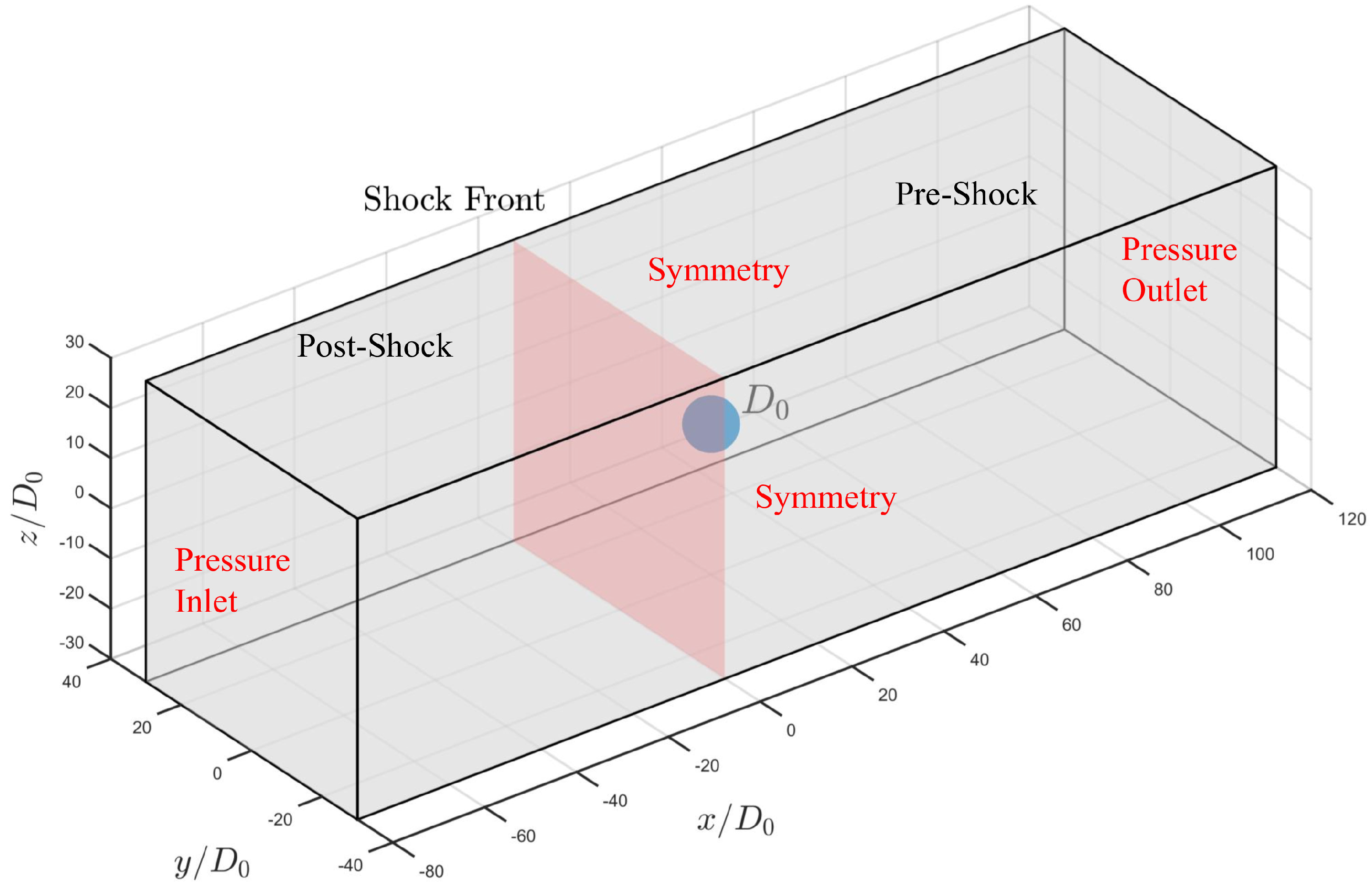
The compressible flow governing equations were solved in a rectangular computational domain given by , where stands for the initial droplet diameter. Based on our previous work [32], this domain size was chosen with the aim of minimizing the influence of boundary conditions. In particular, the ample longitudinal extent allowed the solution not to be affected by the reflected waves from the inlet and outlet boundaries, during the entire duration of the breakup simulation. Fully three-dimensional computations were carried out, without imposing any symmetries or simplifications, in order to capture the non-axisymmetric, complex modulation of the droplet surface and the surrounding airflow field [11]. The simplified flow geometry is drawn in Figure 1, together with a schematic of the physical model at the time instant of the shock impact on the droplet (). The reference coordinates system has the first axis aligned with the stream-wise direction, while the origin corresponds to the leading edge of the spherical water body in its initial position.
Here, different from previous similar studies [12,33], the shock tube flow was not explicitly simulated, but the discontinuous airflow conditions across the moving shock front were directly imposed. The simulations were initiated with the planar shock front being positioned one diameter away from the droplet leading edge, namely, at , separating the two domain sections with post-shock and pre-shock conditions. Note that the shock front and thus the post-shock airflow move in the positive x-axis direction.
4.2. Two-Phase Flow Model
In this study, the two different fluids (liquid water and gas air) were assumed to be immiscible, while using the VOF method for tracking their transient interface [18], which allowed us to approximate the complex boundary between the different phases on the FV grid. According to this methodology, the volume fraction is introduced to distinguish the two phases, where in computational cells with only the liquid phase and in cells with only the gas phase. The time-dependent field variable is evaluated throughout the computational domain by solving the associated continuity equation which is:
Practically, the Navier–Stokes equations are written in terms of the averaged flow fields that are shared by the two different phases. In other words, the compressible flow governing equations are solved for an effective fluid, whose averaged properties are evaluated according to the volume fraction field. The fluid density and viscosity are calculated based on the following arithmetic means:
This way, the fluid properties are representative of either one of the two phases or a mixture of them (where ).
As for the physical model for the surface tension effect, the present computations are performed by employing the continuum surface force (CSF) model proposed by Brackbill and co-workers [34], which is widely used in conjunction with the VOF method for two-phase flow. According to this method, the theoretically infinitely thin interface between the two different fluids is replaced by a finite transition region, wherein a body force supersedes the surface tension force acting at the interface. Thus, the resolved momentum equation contains an additional source term mimicking the effect of surface tension between the two fluids. The mathematical details of the CSF model can be found in the above-mentioned reference.
4.3. Numerical Settings
The two-phase flow simulations were performed using the CFD code ANSYS Fluent, which has been successfully employed in analogous works also by other research groups, for instance, in Ref. [10]. The FV method was used for the discretization of the governing equations, with the conservation principles being directly applied over each computational cell [19]. Also, based on similar numerical studies investigating the droplet aerobreakup, e.g., Ref. [6], the main settings of the selected pressure-based solver were as follows.
The SIMPLEC (semi-implicit method for pressure-linked equations—consistent) procedure was used for handling the pressure–velocity coupling, effectively addressing challenges in resolving the transient interface. The pressure staggering option (PRESTO) scheme was used for pressure discretization. This scheme yields more accurate results by avoiding interpolation errors and pressure gradient assumptions on the boundaries, demonstrating improved performance for problems involving strong body forces like surface tension, high density ratios, and steep pressure gradients. Bounded second-order central differencing was used for the momentum and energy equations, while second-order upwind discretization was employed for the model equations and the continuity equation. As for the FV-based approximation of the latter, the compressive scheme, which is a second-order reconstruction scheme based on the gradient limiter, was applied for the advection term in (13).
The temporal integration was performed using the bounded second-order time integration scheme, where the maximum Courant–Friedrichs–Lewy (CFL) number 0.5 was prescribed. As a result, an average time-step of the order of s was obtained, consistent with similar studies [33]. Moreover, as sketched in Figure 1, pressure inlet and pressure outlet boundary conditions were prescribed in the stream-wise direction, employing the thermo-fluid dynamic variables reported in Table 1, while symmetry conditions were imposed at the four lateral faces of the computational domain, assuming zero normal gradients of all balanced variables.
The mesh generation was carried out by exploiting an inner-outer subdomain partitioning strategy, using the software Pointwise V18.4 R4. The inner subdomain was represented by , containing the deforming water droplet at any time during the simulation. This subdomain was uniformly discretized, while the residual outer subdomain was discretized by an unstructured grid made of tetrahedral cells. The FV mesh in the inner region was dynamically locally refined at the interface between the two phases, following the adaptive mesh refinement (AMR) approach, using the gradient of the liquid volume fraction as the control parameter. For illustration, Figure 2 shows a two-dimensional close-up view of the adaptive spatial grid in the vicinity of the droplet, at three different time instants corresponding to , , and .
5. Results and Discussion
In this section, the results of the three different simulations with different turbulence models are presented and discussed. Both qualitative and quantitative analyses of droplet drift, deformation, and breakup are performed, making a comparison against literature data.
5.1. Droplet Movement and Deformation
The numerical simulation of the early stages of the shock–droplet interaction process is mainly asked to accurately predict the induced kinematics and deformation of the water droplet. These results are essential for understanding the subsequent breakup phase. The droplet kinematics is normally examined by looking at the position and stream-wise velocity of the droplet center-of-mass (CM), which are defined, according to the VOF formulation, as:
and
respectively. The above integrals extending over the overall computational domain inherently include only the contributions from the fluid flow regions that are occupied by the liquid phase, wherein the volume fraction is non-zero. In the following, the displacement and velocity parameters are normalized as and , respectively. It is noteworthy that the above CM displacement does not coincide with the drift of the droplet leading edge [9]. As far as the droplet deformation is concerned, following the usual approach, it is examined by measuring the linear extents of the evolving water body in both the stream-wise direction and cross-stream plane, and , respectively [10].
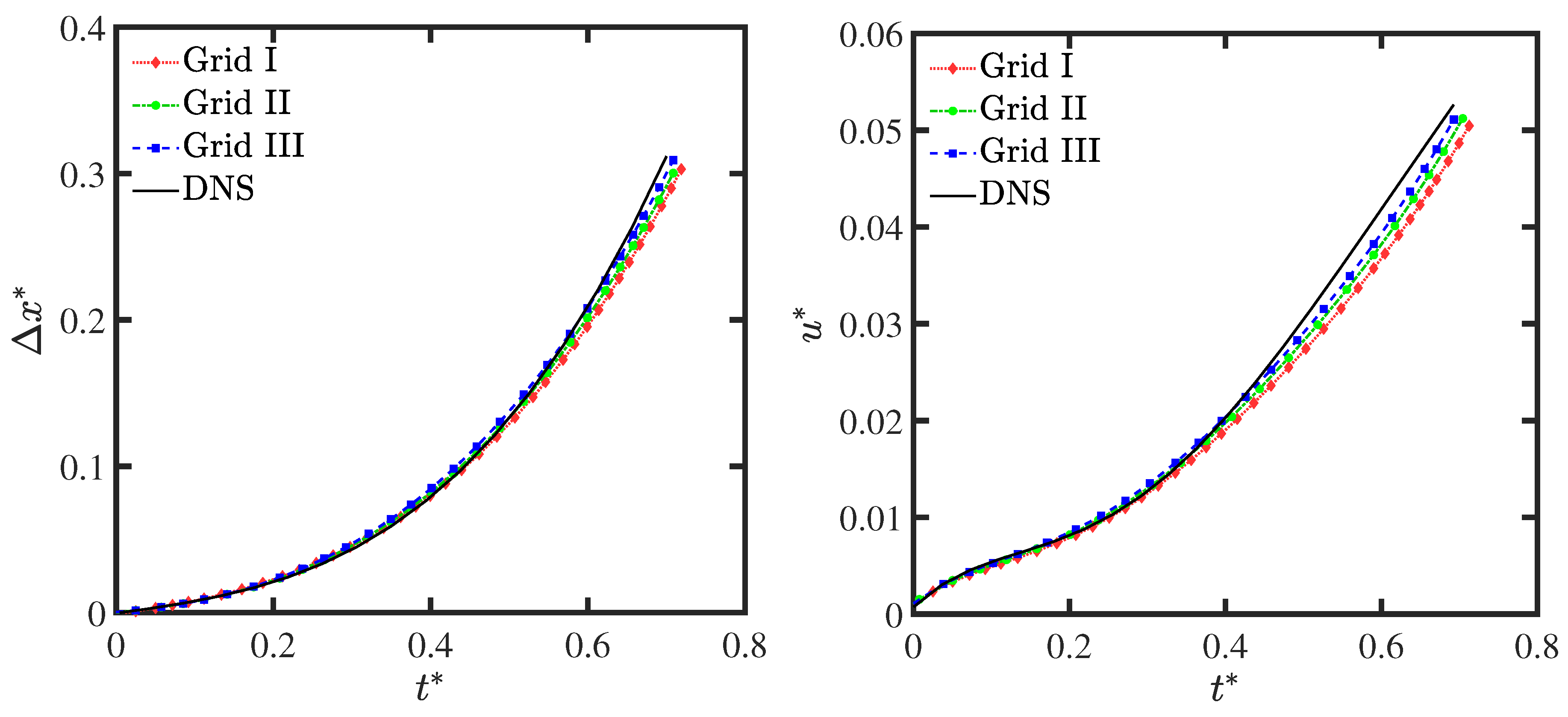
As a preliminary test, the robustness of the computational model proposed in Section 4 was assessed by performing a numerical convergence analysis, for example, for the SRS solution with the SBES approach. Three different calculations were carried out for varying spatial resolution. The associated mesh sizes corresponding to the inner subdomain are tabulated in Table 3, where stands for the minimum linear size of the refined FV grid at the interface. Note that, owing to the prescribed CFL condition, the time integration step was consistently reduced with refining the spatial grid. The highest local resolution resulted in it corresponding to 220 cells per initial diameter, which is still not sufficient for the direct numerical approach [35]. Indeed, the theoretical DNS resolution that is required to reproduce the complete physics of aerobreakup, while capturing all fine-scale effects, makes the problem practically unaffordable, according to the careful estimation made in [11]. On the other hand, the LES approach has been demonstrated to be quite promising for predicting the essential features of aerobreakup with manageable computational complexity [6,10].
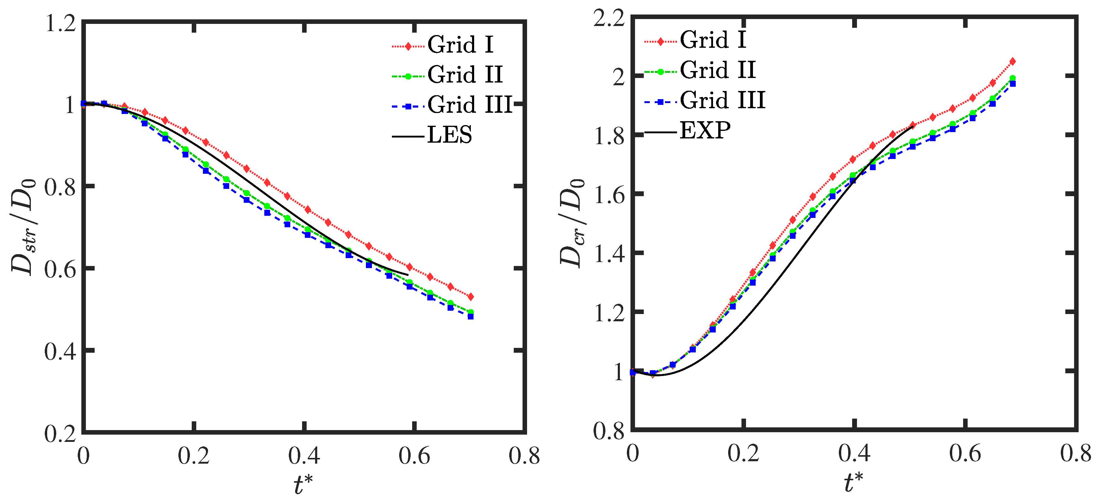
Figure 3 shows the normalized CM displacement and velocity against non-dimensional time for the SBES with different numerical resolutions compared against the high-fidelity solution provided by Meng and Colonius [11]. The latter is assumed hereafter as reference DNS, even though the study was conducted in the inviscid case, without considering the surface tension effect. Apparently, the predicted droplet displacement slightly increases with the numerical resolution, according to what was recently found in Ref. [13]. The accuracy of the prediction improved with increasing the resolution while approaching the reference data. As for deformation parameters, they are depicted in Figure 4, normalized by the initial droplet diameter . Given the hybrid nature of the SBES solution, the numerical resolution has a marked effect on the predicted droplet dimensions. In fact, the LES component of the model becomes more important with the grid refinement, especially at the gas–liquid interface, which allows for a more accurate prediction of the droplet boundary. The present results are consistent with literature data for the aerobreakup of water droplets at similar (but different) conditions. For comparison, either the LES results in Ref. [10], obtained for and atm, or the shock tube experimental findings in Ref. [6], acquired for and , are considered here.
Upon inspection of Figure 3 and Figure 4, the accuracy of the present results does not seem to greatly improve going from Grid II to Grid III. The relative errors associated with the two coarser grids against the finest one, which are evaluated for the different variables at the final instant of the simulations, are summarized in Table 4. Also, looking at these data, the numerical resolution corresponding to Grid III can be regarded as adequate for the present case study. Therefore, the various solutions with different turbulence modeling were obtained using this grid, as presented in the following.
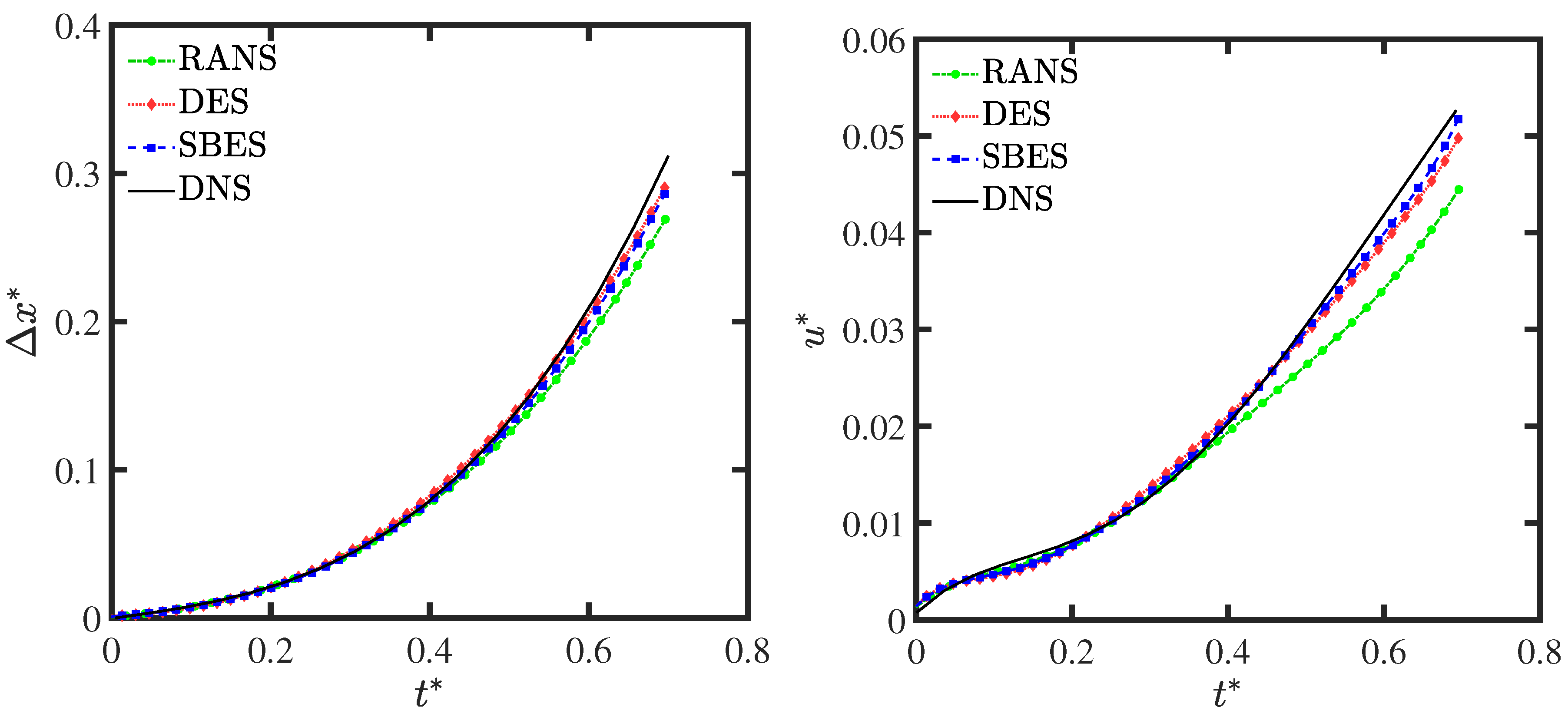
The time histories of the CM displacement and velocity predicted by the three different models, namely, unsteady RANS, DES, and SBES, are depicted in Figure 5. Seemingly, a good agreement is achieved between present solutions and reference DNS data in terms of droplet kinematics. The transient position of the droplet is satisfactorily captured, regardless of the turbulence model, even though the velocity is slightly underestimated. The SRS models give better results compared to RANS, with a small superiority of the SBES approach. Nevertheless, these results are not definitively indicative of the model performance, because the integral parameters (16) and (17) result in being rather insensitive to unsteady small-scale interface structures, which are differently resolved by means of the different methods.
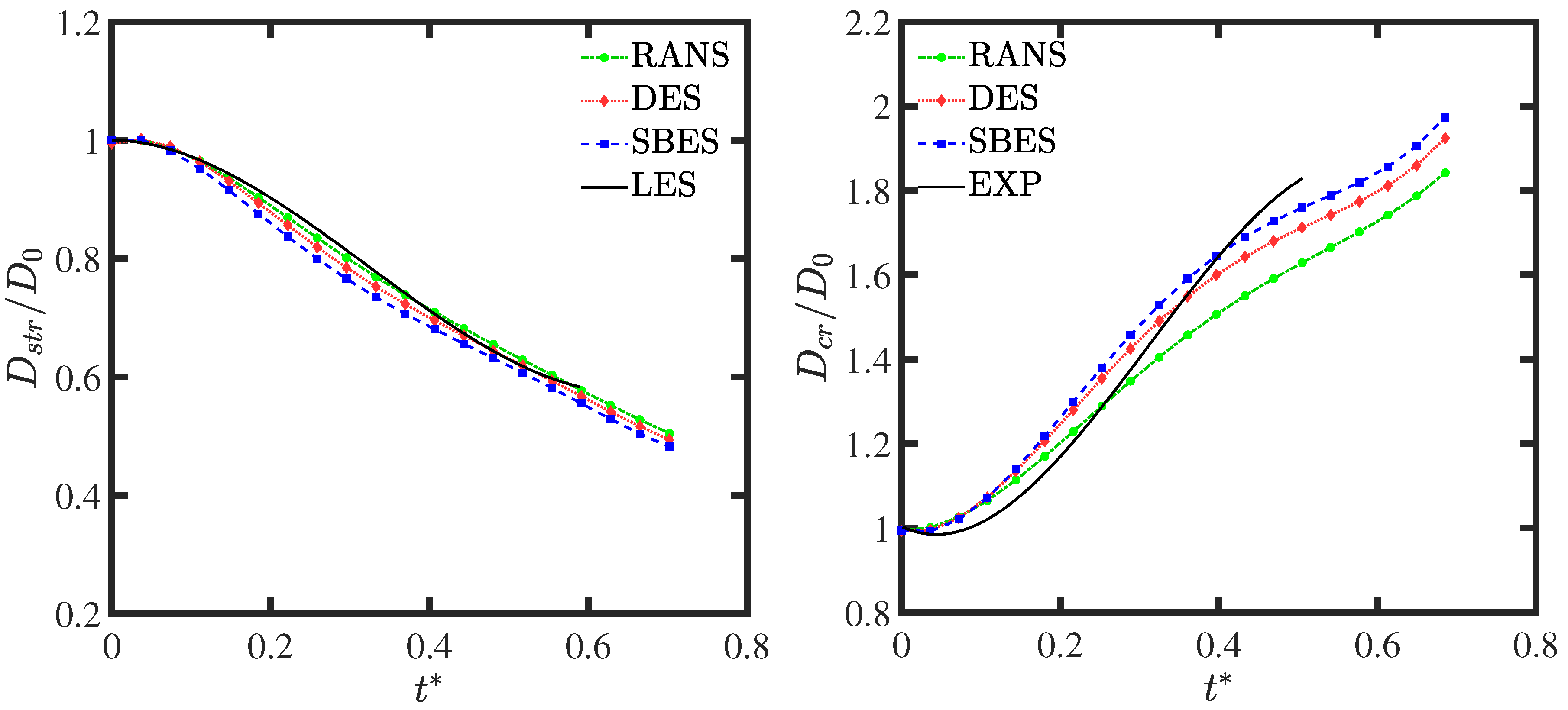
Furthermore, the time histories of the dimensionless cross-stream and stream-wise extents are reported in Figure 6 for the three different models. Initially, the passage of the shock wave does not induce appreciable droplet deformation (), since there exists a characteristic reaction time during which the water body shows no change in shape [7]. After this time has elapsed, the temporal evolution shows a decreasing , along with an increasing , as the parent droplet is continuously compressed, becoming thinner and thinner in the stream-wise direction. Indeed, the water body maintains its coherence, while being flattened under the pressure difference existing between the windward and leeward sides. Moreover, due to the stretching of liquid sheets and ligaments at the periphery of the parent droplet, as demonstrated in the following section, the cross-stream extent is continuously expanding. The present VOF-based computational model provides acceptably accurate predictions for the droplet deformation, though some discrepancies against the reference data exist for the cross-stream extent.
Another important result to be analyzed is represented by the induction time, which is the time it takes for the first sub-droplets to break off from the parent droplet. The normalized values of this parameter predicted by RANS, DES, and SBES solutions are , , and , respectively. Again, the SRS models are able to provide results closer to the experimental findings [24].
5.2. Droplet Breakup Dynamics
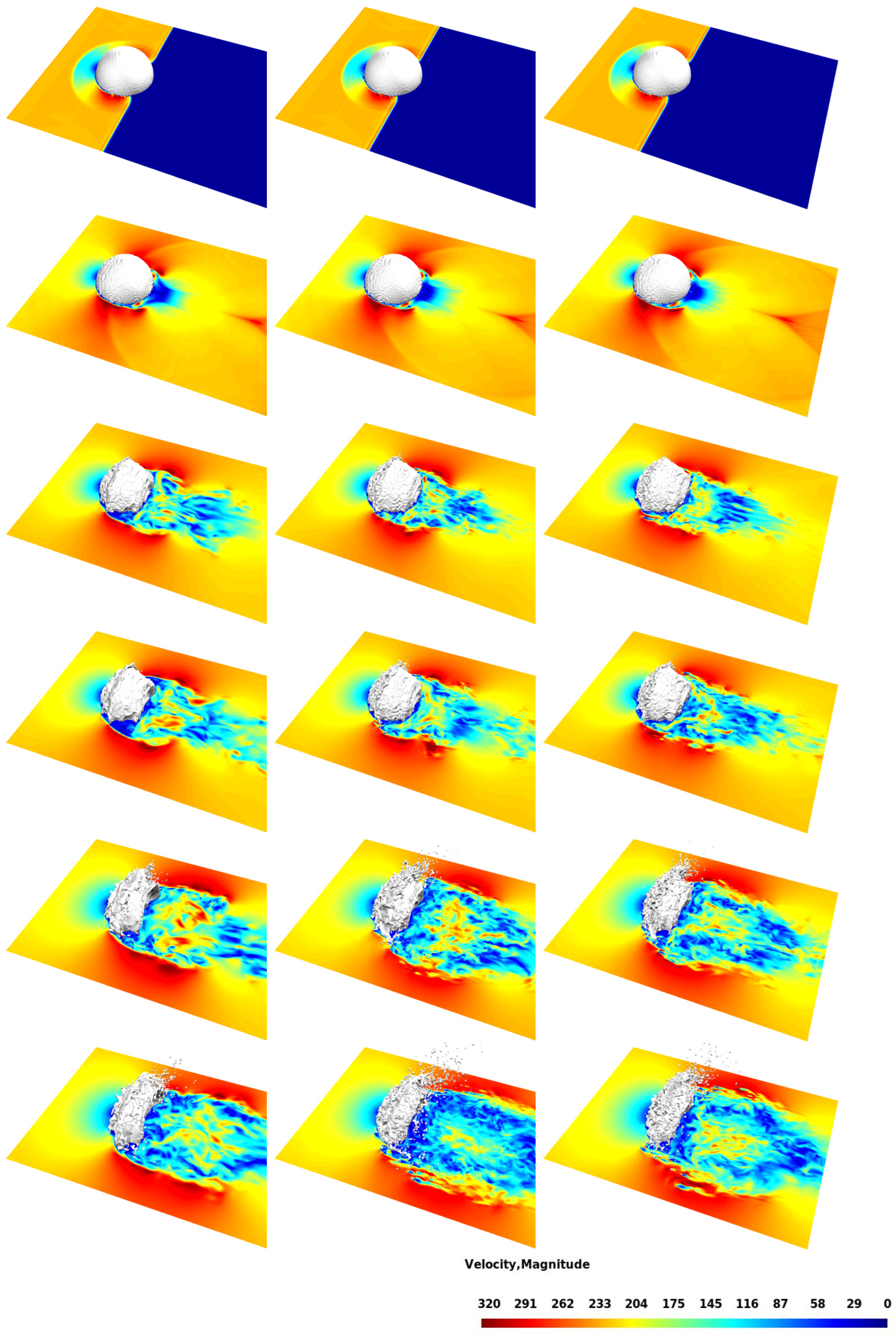
The different phases of the aerobreakup phenomenon are illustrated in Figure 7, by considering the temporal evolution of the air–water interface, along with the associated velocity contours, for the different approaches. The instantaneous shape of the deforming droplet is determined as the one corresponding to the isosurface at for the volume fraction of water, while the contour maps are reported in the plane. Here and in the following, the field magnitude is reported using international system units. The different snapshots correspond to six different time instants in the interval . To correctly visualize the deformation of the water body, the size and position of the zoomed images, reporting the leeward side of the droplet, are exactly the same for each snapshot. Owing to the adopted AMR procedure, the FV mesh is locally refined at the interface between the two immiscible fluids, and the droplet surface appears only very slightly diffuse.
The complex wave dynamics originating from the impact of the moving shock front on the liquid surface is illustrated by the first two rows. The corresponding temporary ambient conditions are rapidly replaced by the post-shock airflow conditions, which mainly influence the kinematics of the droplet, as well as the aerobreakup mechanism. Making a comparison with reference data provided by shock tube experiments, e.g., in Refs. [5,24], the overall breakup dynamics results in it being well captured by the present numerical simulations. As expected at high Weber numbers, owing to the high-speed post-shock airstream in which the water body is immersed, the breakup is governed by the shear-induced surface waves. Indeed, due to the velocity difference across the interface between the two immiscible fluids, KH instability waves are generated on the windward side of the droplet. Initially, despite the shearing action of the surrounding airflow, the parent droplet maintains an almost spherical shape, owing to the relatively strong surface tension force. As time goes on, the KH instabilities become more prominent, while traveling on the droplet surface and merging to form a liquid sheet at the droplet equator. Then, the liquid sheet undergoes localized breakup processes through the nucleation of different holes. The latter phase is accompanied by the recurrent fragmentation of liquid ligaments, with the overall picture corresponding to the SIE breakup mode [9].
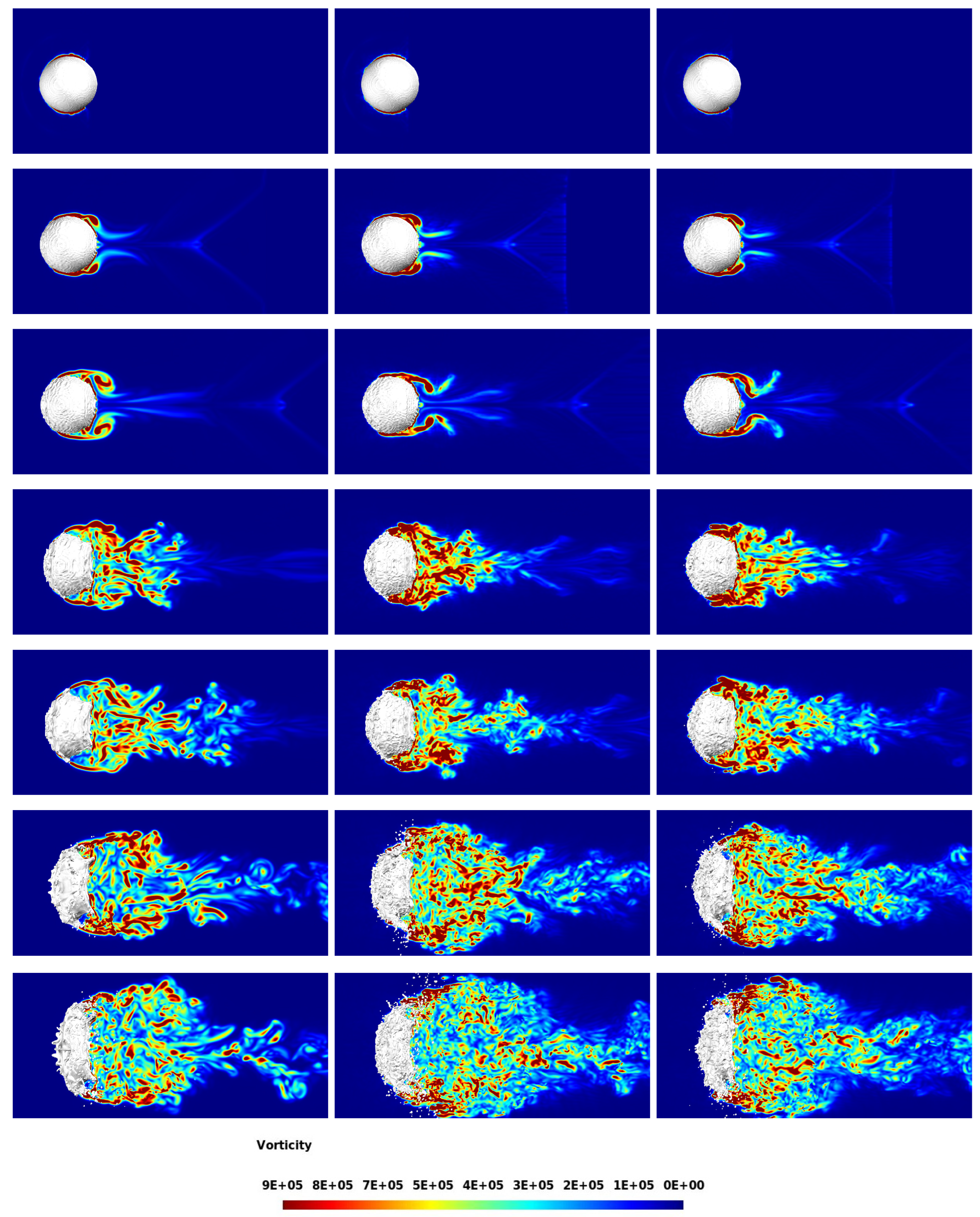
Actually, the above complex two-phase flow evolution is diversely captured by the three different methods. The generation of small-scale motions at the air–water interface, which eventually lead to the formation of unstable interfacial vortical flow patterns, results in them being affected by the turbulence modeling approach, which also influences the characteristic wavelengths and growth rates of the KH instabilities. The small-scale flow features are only partially captured by the unsteady RANS model, whereas both SRS models give solutions that are fully consistent with the results of more sophisticated high-resolution numerical simulations, e.g., Refs. [6,11]. Basically, the scale-resolving capabilities of DES and SBES make these models more effective in reproducing the birth and evolution of two-phase fluid instabilities, as well as the overall breakup mechanism [36]. For instance, this is illustrated in Figure 8, where the vorticity magnitude contours in the proximity of the droplet are drawn at a meridian plane, in the near wake of the droplet. Initially, as the water body is only slightly deformed, the airflow pattern resembles that one around a solid sphere, with the presence of toroidal vortical structures originating from the boundary-layer separation. At later time instants, the very complex wake flow is differently reproduced by the different models. Generally, the SRS solutions exhibit a more three-dimensional character, apparently being able to resolve fine-scale flow structures.
5.3. Turbulence Resolution
When simulating the water droplet aerobreakup, the presence of high velocity gradients at the interface between the two different fluid phases results in the generation of high turbulent fluctuations in both fluids [28]. Due to the very wide range of turbulence scales that are involved, which does not allow for the direct solution of all the turbulent fluctuations, the turbulence modeling procedure plays a key role in this context, together with the appropriate numerical resolution. In principle, differently from RANS, small-scale unsteady structures at the air–water interface may be resolved, at least partially, by means of both SRS methods under investigation.
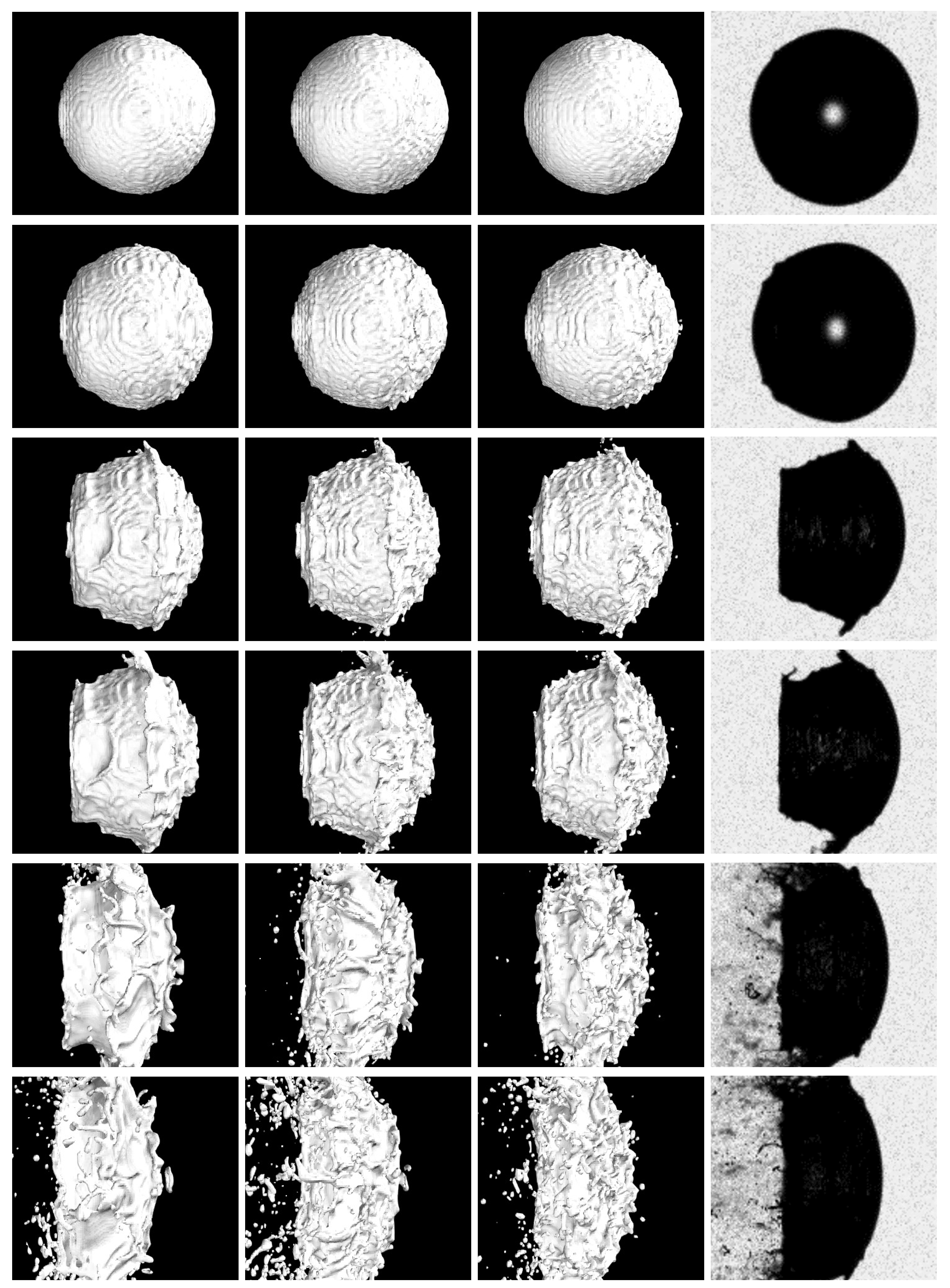
Thus, to assess their scale-resolving capabilities, the three different turbulence models are further examined by making a direct comparison with experimental findings, in terms of time-dependent droplet morphology. In Figure 9, the side views of the deforming droplet in a meridian plane, traced by non-dimensional time, are compared to corresponding experimental images provided by Theofanous and co-workers [37]. By looking at the six different snapshots that are reported in the time interval , the present results acceptably agree with the observations made in the reference experiment, investigating the water droplet breakup at We = 780, with a post-shock flow Mach number of 0.32. Note that, owing to the higher Mach number, the surface instabilities are more pronounced for the present numerical solutions.
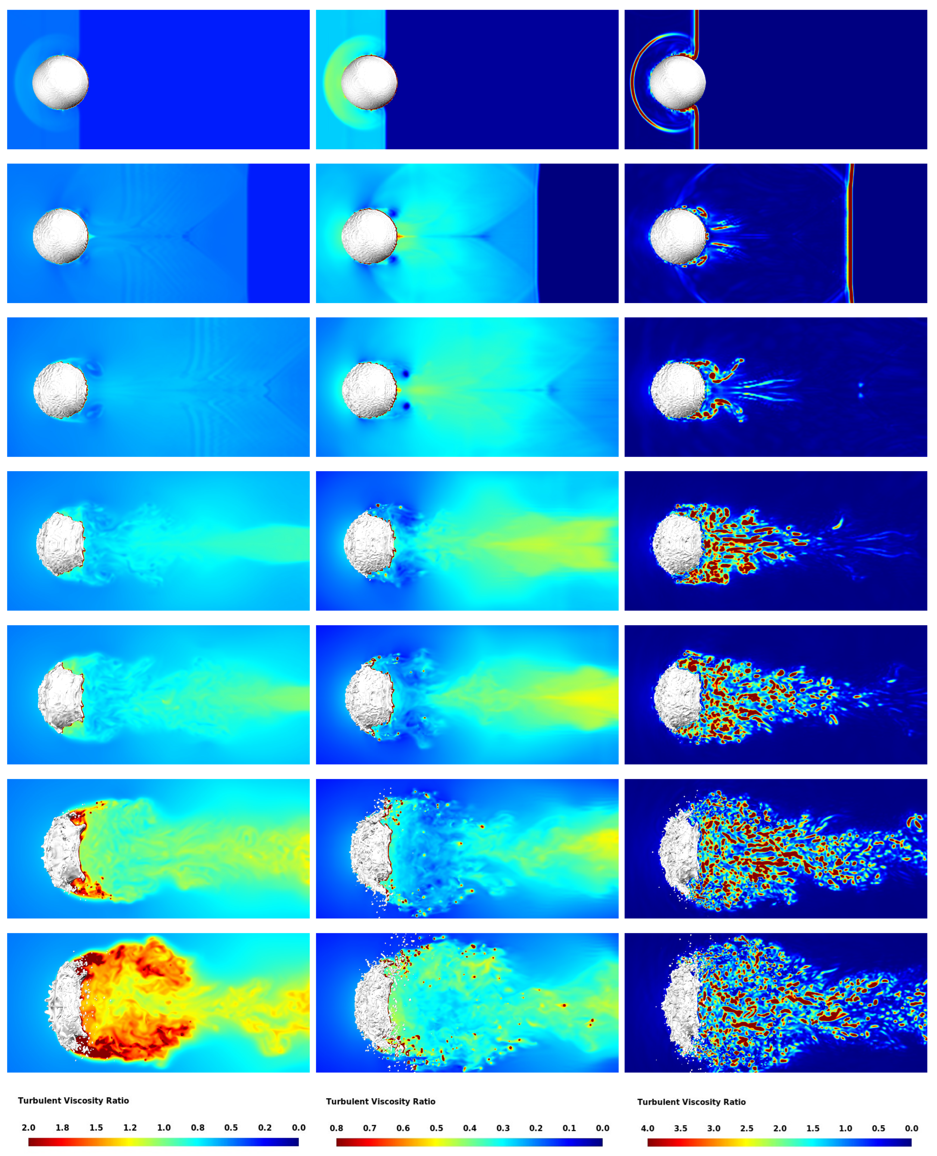
It can be seen that SRS provides more accurate solutions with respect to unsteady RANS. Indeed, the latter approach prevents the formation of certain three-dimensional structures, due to relatively high eddy-viscosity levels, and inherently cannot represent the fine-scale structure of the two-phase flow. On the contrary, the SRS methods locally adjust to the smallest flow scales, producing an eddy-viscosity level low enough to permit the formation of even smaller eddies, until the grid limit is reached. In fact, the modeled turbulent viscosity is distinctively lower for DES with respect to RANS, as illustrated in Figure 10, where the contour maps of the turbulent viscosity ratio are reported against time. As for SBES, though this parameter may locally take high values, the rapidly varying solution shows localized flow regions with LES-like levels of modeled eddy-viscosity.
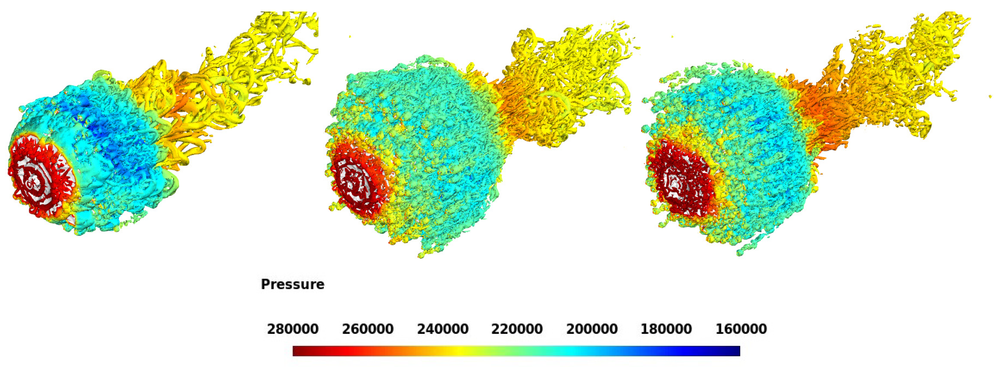
These results suggest that both of the current SRS formulations are capable of accurately reproducing the aerobreakup process by resolving the small-scale turbulent flow structures, with an accuracy comparable to more expensive methods [11]. Naturally, the agreement with both experimental and higher-order numerical data improves with the ability of SRS models to locally switch into the LES-like mode. This is further demonstrated in Figure 11, where the vortical structures in the near wake are visualized in terms of the isosurfaces of the Q-criterion, colored by the pressure field, at a given time instant.
6. Conclusions
Following a fully three-dimensional approach, the early stages of the aerobreakup of a water droplet induced by the interaction with a traveling plane shock wave were numerically simulated. Two different scale-resolving methods were tested along with pure unsteady RANS, namely, the DES and SBES models. In the former case, a single model acts in either RANS or LES mode, depending on the local grid resolution. In the latter case, two separate models for the two different (RANS and LES) components are utilized, by using an enhanced blending function between them. The numerical calculations made use of the VOF technique to model the gas–liquid interface while employing dynamic meshing technology to improve the computational efficiency. The results of the three different approaches were compared with each other, as well as with relevant reference data.
The various computational models were able to predict the droplet kinematics, the interface deformation, and the incipient breakup. Indeed, the two different stages of the process, which are droplet flattening and sheet shearing at the droplet periphery, were correctly simulated, with the findings of wind tunnel experiments as well as higher-fidelity numerical simulations being acceptably reproduced. While the unsteady RANS solution was able to predict the mean flow evolution, confirming previous research findings [32], the turbulence-resolving capability of the more sophisticated SRS models was practically demonstrated. These methods allow us to reproduce localized unsteady small-scale structures that are of crucial importance for the physics of aerobreakup. Definitely, the SRS approach was proven to offer a viable tool for the present complex two-phase turbulent flow application, with affordable computational complexity, which is particularly important from an industrial research perspective. In fact, the computational time for both SRS solutions was increased by only about compared to the unsteady RANS simulation, which required nearly 120 CPU hours using nine computing nodes with 48 cores each, running on an HPC cluster.
The present work is expected to give some guidance for simulating the aerodynamic fragmentation of liquid droplets in engineering applications. It was conducted for a particular benchmark case and represents the proof-of-concept, as further investigations will be performed for varying physical models and different two-phase flow conditions. Moreover, following the idea of Hosseinzadeh-Nik et al. [38], future developments for the numerical simulation of shock-induced droplet breakup will deal with wavelet transform-based adaptive numerical methods [39], which have recently been extended to supersonic turbulent flows [40]. Specifically, the application of promising multiscale RANS-based modeling techniques will be explored, as they were proven to possess a pronounced potentiality for turbulence scale-resolving simulation [41].
Finally, the SRS methods adopted here can be also used to estimate the air density and velocity fields actually experienced by the droplet, allowing for more accurate evaluations of classical correlations for breakup times derived from planar shock–drop interactions, for instance, in aerospace engineering research [42].
Author Contributions
Conceptualization, G.D.; methodology, G.D.; validation, V.R. and G.D.; investigation, V.R. and G.D.; resources, V.R. and G.D.; data curation, V.R.; writing—original draft preparation, G.D.; writing—review and editing, G.D.; visualization, V.R.; supervision, G.D. All authors read and agreed to the published version of the manuscript.
Funding
This research received no external funding.
Institutional Review Board Statement
Not applicable.
Informed Consent Statement
Not applicable.
Data Availability Statement
Data are contained within the article.
Acknowledgments
The authors thank Emeritus Theo G. Theofanous, University of California at Santa Barbara, for kindly providing the experimental images reported in Figure 9. The authors acknowledge the CINECA award under the ISCRA initiative for the availability of high-performance computing resources (Project HP10CDJIHF).
Conflicts of Interest
The authors declare no conflicts of interest.
Abbreviations
The following abbreviations are used in this manuscript:
| AMR | adaptive mesh refinement |
| CFL | Courant–Friedrichs–Lewy (number) |
| CM | center-of-mass |
| CSF | continuum surface force (model) |
| DES | detached-eddy simulation |
| DNS | direct numerical simulation |
| FV | finite volume (method) |
| HPC | high-performance computing |
| KH | Kelvin–Helmholtz (instability) |
| LES | large-eddy simulation |
| RANS | Reynolds-averaged Navier–Stokes (equations) |
| RTP | Rayleigh–Taylor piercing |
| SBES | stress-blended eddy simulation |
| SGS | subgrid-scale (model) |
| SIE | shear-induced entrainment |
| SRS | scale-resolving simulation |
| SST | shear-stress transport (model) |
| VOF | volume-of-fluid (method) |
| WALE | wall-adapting local eddy-viscosity (model) |
References
- Theofanous, T.G.; Li, G. On the physics of aerobreakup. Phys. Fluids 2008, 20, 052103. [Google Scholar] [CrossRef]
- Guildenbecher, D.R.; López-Rivera, C.; Sojka, P.E. Secondary atomization. Exp. Fluids 2009, 46, 371–402. [Google Scholar] [CrossRef]
- Ranger, A.A.; Nicholls, J.A. Aerodynamic shattering of liquid drops. In Proceedings of the 6th AIAA Aerospace Sciences Meeting, New York, NY, USA, 22–24 January 1968. [Google Scholar]
- Moylan, B.; Landrum, B.; Russell, G. Investigation of the physical phenomena associated with rain impacts on supersonic and hypersonic flight vehicles. Procedia Eng. 2013, 58, 223–231. [Google Scholar] [CrossRef]
- Wang, Z.; Hopfes, T.; Giglmaier, M.; Adams, N.A. Effect of Mach number on droplet aerobreakup in shear stripping regime. Exp. Fluids 2020, 61, 193. [Google Scholar] [CrossRef] [PubMed]
- Poplavski, S.; Minakov, A.; Shebeleva, A.; Boiko, V. On the interaction of water droplet with a shock wave: Experiment and numerical simulation. Int. J. Multiph. Flow 2020, 127, 103273. [Google Scholar] [CrossRef]
- Engel, O.G. Fragmentation of water drops in the zone behind an air shock. J. Res. Nat. Bur. Stand. 1958, 60, 245–280. [Google Scholar] [CrossRef]
- Hinze, J.O. Fundamentals of the hydrodynamic mechanism of splitting in dispersion processes. AIChE J. 1955, 1, 289–295. [Google Scholar] [CrossRef]
- Theofanous, T.G. Aerobreakup of Newtonian and viscoelastic liquids. Annu. Rev. Fluid Mech. 2011, 43, 661–690. [Google Scholar] [CrossRef]
- Zhu, W.; Zhao, N.; Jia, X.; Chen, X.; Zheng, H. Effect of airflow pressure on the droplet breakup in the shear breakup regime. Phys. Fluids 2021, 33, 053309. [Google Scholar] [CrossRef]
- Meng, J.C.; Colonius, T. Numerical simulation of the aerobreakup of a water droplet. J. Fluid Mech. 2018, 835, 1108–1135. [Google Scholar] [CrossRef]
- Rossano, V.; Cittadini, A.; De Stefano, G. Computational evaluation of shock wave interaction with a liquid droplet. Appl. Sci. 2022, 12, 1349. [Google Scholar] [CrossRef]
- Wei, Y.; Dong, R.; Zhang, Y.; Liang, S. Study on the interface instability of a shock wave-sub-millimeter liquid droplet interface and a numerical investigation of its breakup. Appl. Sci. 2023, 13, 13283. [Google Scholar] [CrossRef]
- Ge, X.; Vasilyev, O.V.; De Stefano, G.; Hussaini, M.Y. Wavelet-based adaptive unsteady Reynolds-averaged Navier-Stokes computations of wall-bounded internal and external compressible turbulent flows. In Proceedings of the 56th AIAA Aerospace Sciences Meeting, Kissimme, FL, USA, 8–12 January 2018. [Google Scholar]
- Menter, F.R.; Hüppe, A.; Matyushenko, A.; Kolmogorov, D. An Overview of Hybrid RANS-LES Models Developed for Industrial CFD. Appl. Sci. 2021, 11, 2459. [Google Scholar] [CrossRef]
- Strelets, M. Detached eddy simulation of massively separated flows. In Proceedings of the 39th AIAA Aerospace Sciences Meeting, Reno, NV, USA, 8–11 January 2001. [Google Scholar]
- Menter, F. Stress-Blended Eddy Simulation (SBES)—A New Paradigm in Hybrid RANS-LES Modeling. In Progress in Hybrid RANS-LES Modelling, Proceedings of the Papers Contributed to the 6th Symposium on Hybrid RANS-LES Methods, Strasbourg, France, 26–28 September 2016; Hoarau, Y., Peng, S.-H., Schwamborn, D., Revell, A., Eds.; Springer: Cham, Switzerland, 2018; pp. 27–37. [Google Scholar]
- Hirt, C.W.; Nichols, B.D. Volume of fluid (VOF) method for the dynamics of free boundaries. J. Comput. Phys. 1981, 39, 201–225. [Google Scholar] [CrossRef]
- Denaro, F.M.; De Stefano, G. A new development of the dynamic procedure in large-eddy simulation based on a finite volume integral approach. Application to stratified turbulence. Theoret. Comput. Fluid Dyn. 2011, 25, 315–355. [Google Scholar] [CrossRef]
- Igra, D.; Takayama, K. Investigation of aerodynamic breakup of a cylindrical water droplet. At. Sprays 2001, 11, 167–185. [Google Scholar]
- Shyue, K. A fluid-mixture type algorithm for barotropic two-fluid flow problems. J. Comput. Phys. 1998, 200, 718–748. [Google Scholar] [CrossRef]
- Sembian, S.; Liverts, M.; Tillmark, N.; Apazidis, N. Plane shock wave interaction with a cylindrical water column. Phys. Fluids 2016, 28, 056102. [Google Scholar] [CrossRef]
- Rossano, V.; De Stefano, G. Computational evaluation of shock wave interaction with a cylindrical water column. Appl. Sci. 2021, 11, 4934. [Google Scholar] [CrossRef]
- Sharma, S.; Singh, A.P.; Rao, S.S.; Kumar, A.; Basu, S. Shock induced aerobreakup of a droplet. J. Fluid Mech. 2021, 929, A27. [Google Scholar] [CrossRef]
- Menter, F.R. Two-equation eddy-viscosity turbulence models for engineering applications. AIAA J. 1994, 32, 1598–1605. [Google Scholar] [CrossRef]
- Menter, F.R. Review of the shear-stress transport turbulence model experience from an industrial perspective. Int. J. Comput. Fluid Dyn. 2009, 23, 305–316. [Google Scholar] [CrossRef]
- Wilcox, D.C. Turbulence Modeling for CFD; DCW Industries, Inc.: La Cañada, CA, USA, 2006. [Google Scholar]
- Polansky, J.; Schmelter, S. Implementation of turbulence damping in the OpenFOAM multiphase flow solver interFoam. Arch. Thermodyn. 2022, 43, 21–43. [Google Scholar]
- Nicoud, F.; Ducros, F. Subgrid-scale stress modelling based on the square of the velocity gradient tensor. Flow Turbul. Combust. 1999, 62, 183–200. [Google Scholar] [CrossRef]
- Chode, K.K.; Viswanathan, H.; Chow, K.; Reese, H. Investigating the aerodynamic drag and noise characteristics of a standard squareback vehicle with inclined side-view mirror configurations using a hybrid computational aeroacoustics (CAA) approach. Phys. Fluids 2023, 35, 075148. [Google Scholar] [CrossRef]
- Salomone, T.; Piomelli, U.; De Stefano, G. Wall-modeled and hybrid large-eddy simulations of the flow over roughness strips. Fluids 2023, 8, 10. [Google Scholar] [CrossRef]
- Rossano, V.; De Stefano, G. Hybrid VOF-Lagrangian CFD modeling of droplet aerobreakup. Appl. Sci. 2022, 12, 8302. [Google Scholar] [CrossRef]
- Zhu, W.; Zheng, H.; Zhao, N. Numerical investigations on the deformation and breakup of an n–decane droplet induced by a shock wave. Phys. Fluids 2022, 34, 063306. [Google Scholar] [CrossRef]
- Brackbill, J.U.; Kothe, D.B.; Zemach, C. A continuum method for modeling surface tension. J. Comput. Phys. 1992, 100, 335–354. [Google Scholar] [CrossRef]
- Chang, C.H.; Deng, X.; Theofanous, T.G. Direct numerical simulation of interfacial instabilities: A consistent, conservative, all-speed, sharp-interface method. J. Comput. Phys. 2013, 242, 946–990. [Google Scholar] [CrossRef]
- Boiko, V.M.; Poplavski, S.V. Experimental study of two types of stripping breakup of a drop in the flow behind the shock wave. Combust. Explos. Shock Waves 2012, 48, 440–445. [Google Scholar] [CrossRef]
- Theofanous, T.G.; Mitkin, V.V.; Ng, C.L.; Chang, C.H.; Deng, X.; Sushchikh, S. The physics of aerobreakup. II. Viscous liquids. Phys. Fluids 2012, 24, 022104. [Google Scholar] [CrossRef]
- Hosseinzadeh-Nik, Z.; Aslani, M.; Owkes, M.; Regele, J.D. Numerical simulation of a shock wave impacting a droplet using the adaptive wavelet-collocation method. In Proceedings of the ILASS-Americas 28th Annual Conference on Liquid Atomization and Spray Systems, Dearborn, MI, USA, 15–18 May 2016. [Google Scholar]
- Ge, X.; De Stefano, G.; Hussaini, M.Y.; Vasilyev, O.V. Wavelet-based adaptive eddy-resolving methods for modeling and simulation of complex wall-bounded compressible turbulent flows. Fluids 2021, 6, 331. [Google Scholar] [CrossRef]
- De Stefano, G.; Brown-Dymkoski, E.; Vasilyev, O.V. Wavelet-based adaptive large-eddy simulation of supersonic channel flow. J. Fluid Mech. 2020, 901, A13. [Google Scholar] [CrossRef]
- Ge, X.; Vasilyev, O.V.; De Stefano, G.; Hussaini, M.Y. Wavelet-based adaptive unsteady Reynolds-averaged Navier-Stokes simulations of wall-bounded compressible turbulent flows. AIAA J. 2020, 58, 1529–1549. [Google Scholar] [CrossRef]
- Daniel, K.A.; Guildenbecher, D.R.; Delgado, P.M.; White, G.E.; Reardon, S.M.; Stauffacher, H.L.; Beresh, S.J. Drop interactions with the conical shock structure generated by a Mach 4.5 projectile. AIAA J. 2023, 61, 2347–2355. [Google Scholar] [CrossRef]
Figure 1.
Computational domain, along with a schematic of the physical model at , and boundary conditions.
Figure 1.
Computational domain, along with a schematic of the physical model at , and boundary conditions.

Figure 2.
Two-dimensional close-up view of the adaptive spatial grid at three different time instants.
Figure 2.
Two-dimensional close-up view of the adaptive spatial grid at three different time instants.

Figure 3.
Normalized CM displacement (left) and velocity (right) against time: SBES solution with varying numerical resolution, compared to DNS data [11].
Figure 3.
Normalized CM displacement (left) and velocity (right) against time: SBES solution with varying numerical resolution, compared to DNS data [11].

Figure 4.
Stream-wise (left) and cross-stream (right) linear extents of the deforming droplet against time: SBES solution with varying numerical resolution, compared to reference LES [10] or experimental [6] data.

Figure 5.
Normalized CM displacement (left) and velocity (right) against time: different solutions for varying turbulence modeling, compared to DNS data [11].
Figure 5.
Normalized CM displacement (left) and velocity (right) against time: different solutions for varying turbulence modeling, compared to DNS data [11].

Figure 6.
Stream-wise (left) and cross-stream (right) linear extents of the deforming droplet against time: different solutions for varying turbulence modeling, compared to reference LES [10] or experimental [6] data.

Figure 7.
Droplet surface (leeward view) and velocity contours at the plane, for RANS, DES, and SBES solutions (from left to right), against time. The different rows correspond to , , , , , and (from top to bottom).
Figure 7.
Droplet surface (leeward view) and velocity contours at the plane, for RANS, DES, and SBES solutions (from left to right), against time. The different rows correspond to , , , , , and (from top to bottom).

Figure 8.
Contour maps of vorticity magnitude at meridian plane, for RANS, DES, and SBES (from left to right), against time. Different rows correspond to , , , , , , and (from top to bottom).
Figure 8.
Contour maps of vorticity magnitude at meridian plane, for RANS, DES, and SBES (from left to right), against time. Different rows correspond to , , , , , , and (from top to bottom).

Figure 9.
Droplet morphology (lateral view) predicted by RANS, DES, and SBES, compared to corresponding experimental images [37] (from left to right), against time. Different rows correspond to , , , , , and (from top to bottom), while airstream is from right to left.
Figure 9.
Droplet morphology (lateral view) predicted by RANS, DES, and SBES, compared to corresponding experimental images [37] (from left to right), against time. Different rows correspond to , , , , , and (from top to bottom), while airstream is from right to left.

Figure 10.
Contour maps of turbulent viscosity ratio at meridian plane, for RANS, DES, and SBES (from left to right), against time. Different rows correspond to , , , , , , and (from top to bottom).
Figure 10.
Contour maps of turbulent viscosity ratio at meridian plane, for RANS, DES, and SBES (from left to right), against time. Different rows correspond to , , , , , , and (from top to bottom).

Figure 11.
Isosurfaces of Q-criterion at , colored by pressure, for RANS, DES, and SBES (from left to right).
Figure 11.
Isosurfaces of Q-criterion at , colored by pressure, for RANS, DES, and SBES (from left to right).


Table 1.
Physical model: airflow conditions.
| Parameter | Symbol | Pre-Shock | Post-Shock |
|---|---|---|---|
| Pressure (atm) | |||
| Temperature (K) | 293 | 381 | |
| Density () | |||
| Viscosity (dynamic) () | |||
| Velocity (m/s) | 0 | 226 |
Table 2.
Physical model: two-phase flow parameters.
| Parameter | Symbol | Value |
|---|---|---|
| Shock Mach number | ||
| Droplet diameter (mm) | ||
| Mach number | ||
| Reynolds number | ||
| Ohnesorge number | ||
| Weber number | ||
| Density ratio | 460 | |
| Viscosity ratio | 46 | |
| Timescale () | 455 |
Table 3.
Different grid resolutions.
| Denomination | Size | Resolution ( ) |
|---|---|---|
| Grid I | ||
| Grid II | ||
| Grid III |
Table 4.
Relative errors against the finest grid.
| Denomination | Error | Error | Error | Error |
|---|---|---|---|---|
| Grid I | ||||
| Grid II |
Disclaimer/Publisher’s Note: The statements, opinions and data contained in all publications are solely those of the individual author(s) and contributor(s) and not of MDPI and/or the editor(s). MDPI and/or the editor(s) disclaim responsibility for any injury to people or property resulting from any ideas, methods, instructions or products referred to in the content. |
© 2024 by the authors. Licensee MDPI, Basel, Switzerland. This article is an open access article distributed under the terms and conditions of the Creative Commons Attribution (CC BY) license (https://creativecommons.org/licenses/by/4.0/).
Share and Cite
MDPI and ACS Style
Rossano, V.; De Stefano, G. Scale-Resolving Simulation of Shock-Induced Aerobreakup of Water Droplet. Computation 2024, 12, 71. https://doi.org/10.3390/computation12040071
AMA Style
Rossano V, De Stefano G. Scale-Resolving Simulation of Shock-Induced Aerobreakup of Water Droplet. Computation. 2024; 12(4):71. https://doi.org/10.3390/computation12040071
Chicago/Turabian StyleRossano, Viola, and Giuliano De Stefano. 2024. "Scale-Resolving Simulation of Shock-Induced Aerobreakup of Water Droplet" Computation 12, no. 4: 71. https://doi.org/10.3390/computation12040071
Note that from the first issue of 2016, this journal uses article numbers instead of page numbers. See further details here.