
Application of Machine Learning to Predict Blockage in Multiphase Flow

Abstract
1. Introduction
2. Methodology
2.1. Experiments
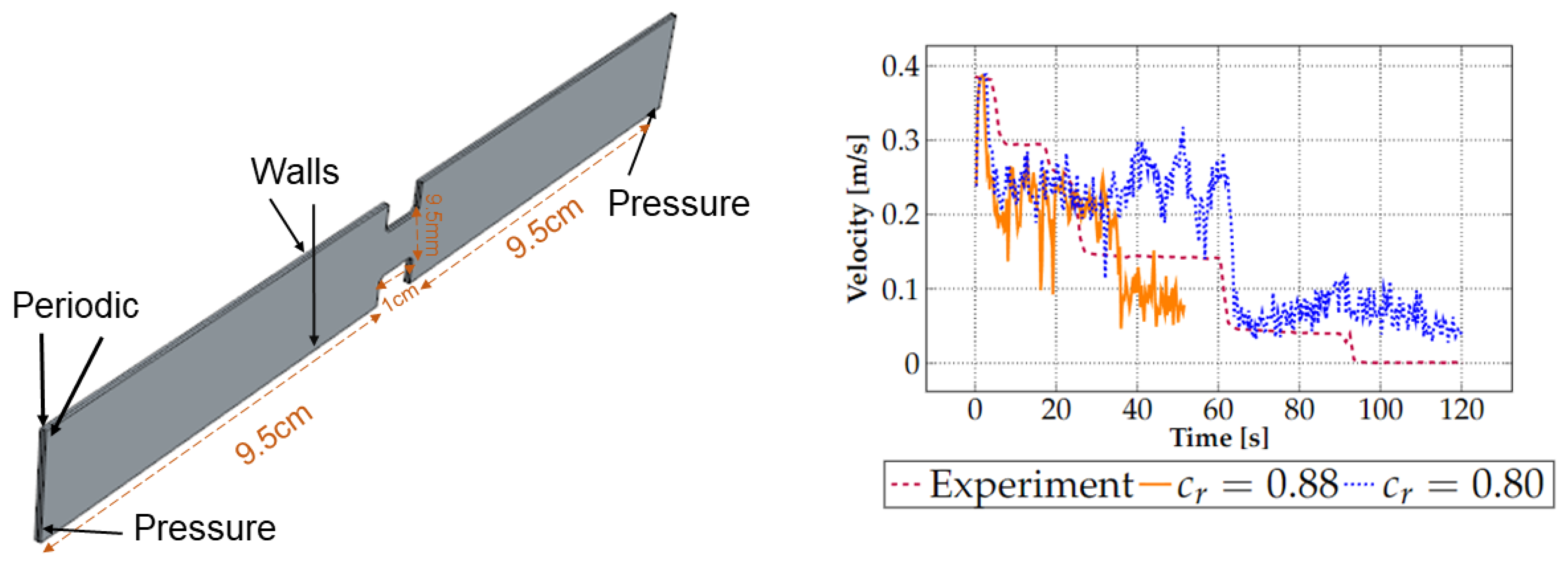
2.2. CFD-DEM Model
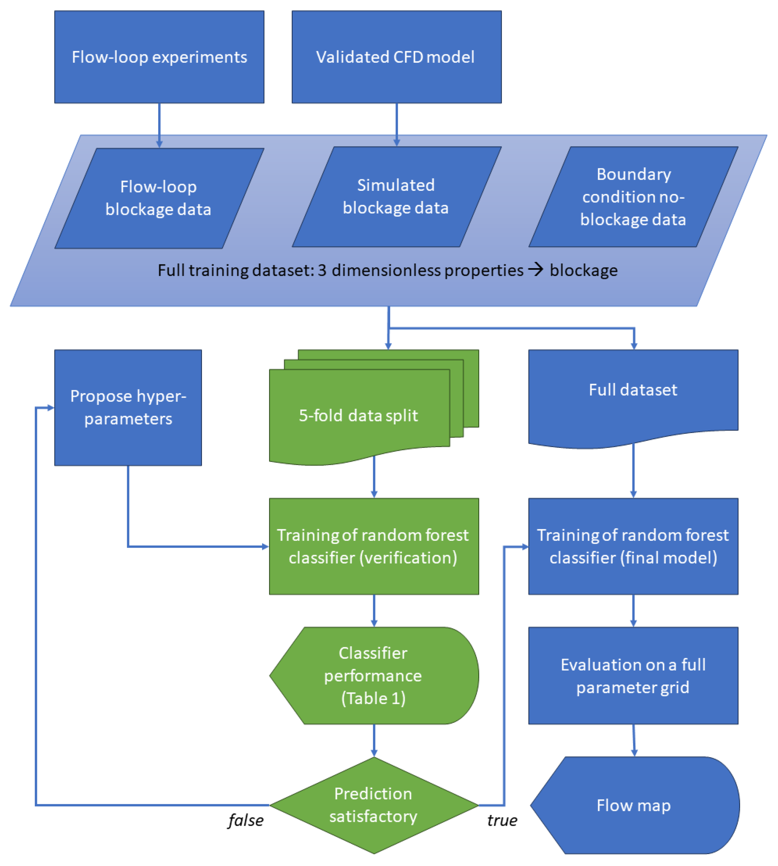
2.3. Machine Learning
3. Results
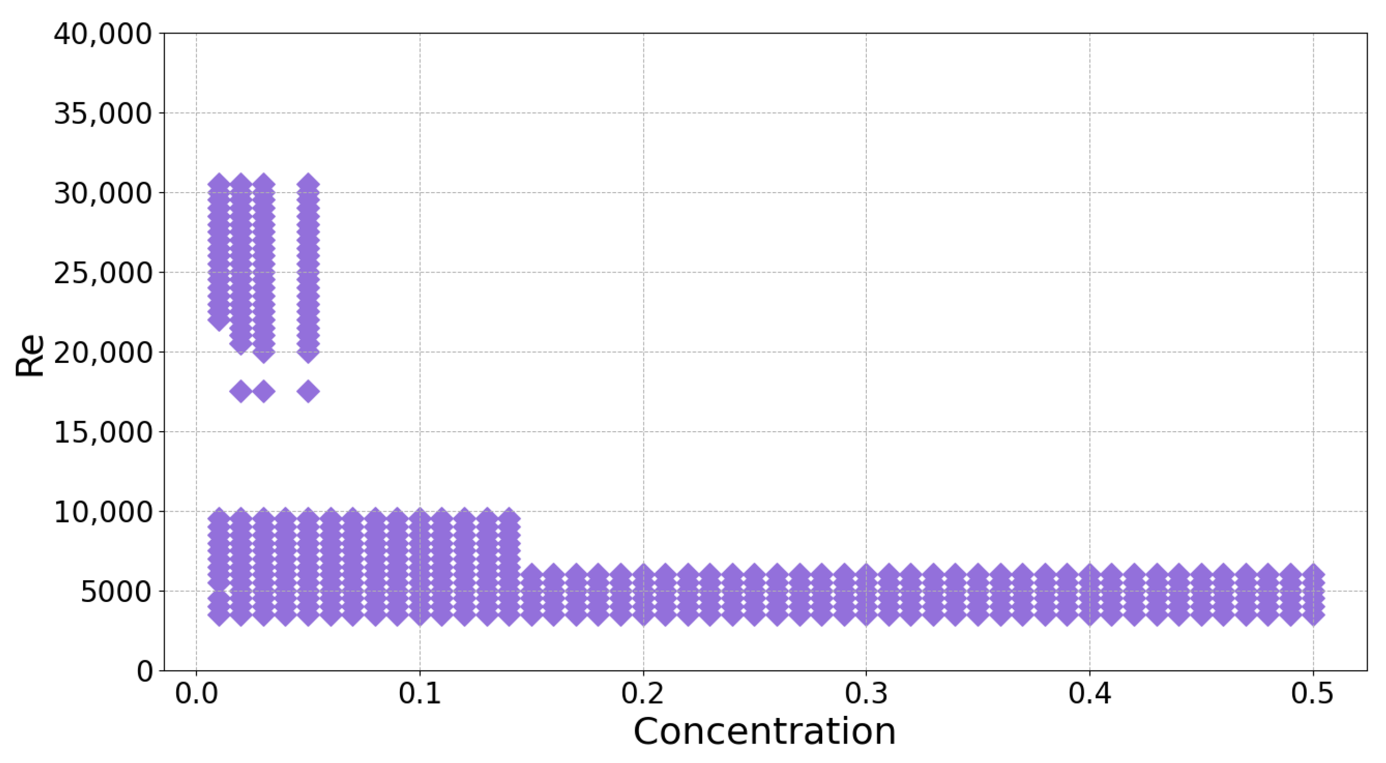
3.1. Machine Learning
Dataset
3.2. Experiments and CFD-DEM Model
3.2.1. Validation
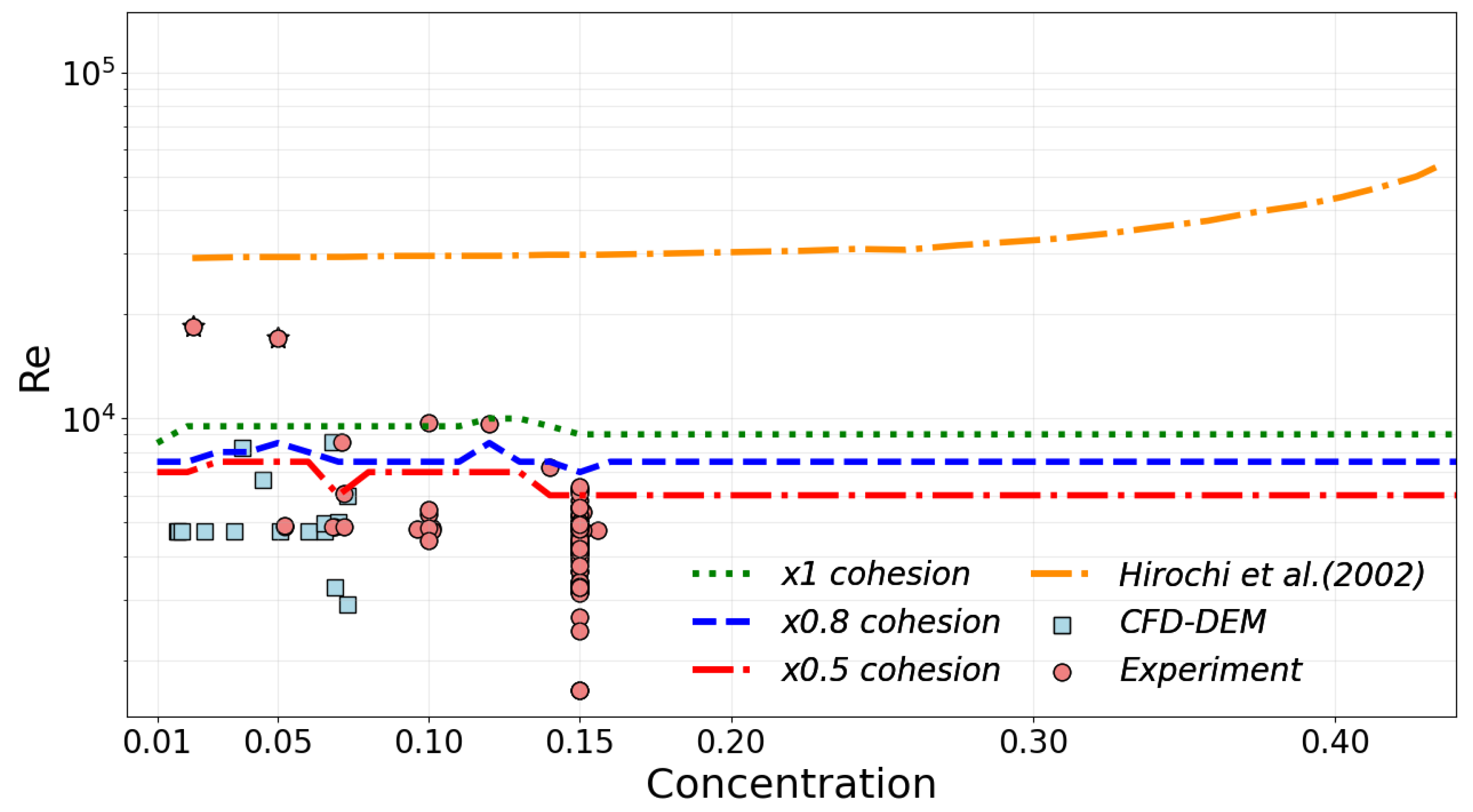
3.2.2. Results
4. Conclusions
Author Contributions
Funding
Data Availability Statement
Conflicts of Interest
References
- Lal, B.; Bavoh, C.B.; Sayani, J.K.S. Machine Learning and Flow Assurance in Oil and Gas Production; Springer Nature: Berlin/Heidelberg, Germany, 2023. [Google Scholar]
- Manikonda, K.; Hasan, A.R.; Obi, C.E.; Islam, R.; Sleiti, A.K.; Abdelrazeq, M.W.; Rahman, M.A. Application of Machine Learning Classification Algorithms for Two-Phase Gas-Liquid Flow Regime Identification. In Proceedings of the Abu Dhabi International Petroleum Exhibition and Conference, Abu Dhabi, United Arab Emirates, 2–5 October 2021; p. D041S121R004. [Google Scholar]
- Hasan, A.R.; Kabir, C.S.; Sarica, C. Fluid Flow and Heat Transfer in Wellbores; Society of Petroleum Engineers: Richardson, TX, USA, 2018. [Google Scholar]
- Alhashem, M. Machine learning classification model for multiphase flow regimes in horizontal pipes. In Proceedings of the International Petroleum Technology Conference, Beijing, China, 28 March 2020; p. D023S042R001. [Google Scholar]
- Chaari, M.; Seibi, A.C.; Hmida, J.B.; Fekih, A. An optimized artificial neural network unifying model for steady-state liquid holdup estimation in two-phase gas–liquid flow. J. Fluids Eng. 2018, 140, 101301. [Google Scholar] [CrossRef]
- Qin, H.; Srivastava, V.; Wang, H.; Zerpa, L.E.; Koh, C.A. Machine learning models to predict gas hydrate plugging risks using flowloop and field data. In Proceedings of the Offshore Technology Conference, Houston, TX, USA, 16–19 August 2019; p. D011S010R003. [Google Scholar]
- Evans, J.H. Dimensional analysis and the Buckingham Pi theorem. Am. J. Phys. 1972, 40, 1815–1822. [Google Scholar] [CrossRef]
- Wang, J.; Wang, Q.; Meng, Y.; Yao, H.; Zhang, L.; Jiang, B.; Liu, Z.; Zhao, J.; Song, Y. Flow characteristic and blockage mechanism with hydrate formation in multiphase transmission pipelines: In-situ observation and machine learning predictions. Fuel 2022, 330, 125669. [Google Scholar] [CrossRef]
- Muller, A.C.; Guido, S. Introduction to Machine Learning with Python; O’Reilly: Farnham, UK, 2017. [Google Scholar]
- Kim, J.; Han, S.; Seo, Y.; Moon, B.; Lee, Y. The development of an AI-based model to predict the location and amount of wax in oil pipelines. J. Pet. Sci. Eng. 2022, 209, 109813. [Google Scholar] [CrossRef]
- Amar, M.N.; Ghahfarokhi, A.J.; Ng, C.S.W. Predicting wax deposition using robust machine learning techniques. Petroleum 2022, 8, 167–173. [Google Scholar] [CrossRef]
- Ahmadi, M. Data-driven approaches for predicting wax deposition. Energy 2023, 265, 126296. [Google Scholar] [CrossRef]
- Struchalin, P.G.; Øye, V.H.; Kosinski, P.; Hoffmann, A.C.; Balakin, B.V. Flow loop study of a cold and cohesive slurry. Pressure drop and formation of plugs. Fuel 2023, 332, 126061. [Google Scholar] [CrossRef]
- Hirochi, T.; Yamada, S.; Shintate, T.; Shirakashi, M. Ice/water slurry blocking phenomenon at a tube orifice. Ann. N. Y. Acad. Sci. 2002, 972, 171–176. [Google Scholar] [CrossRef] [PubMed]
- Saparbayeva, N.; Balakin, B.V. CFD-DEM model of plugging in flow with cohesive particles. Sci. Rep. 2023, 13, 17188. [Google Scholar] [CrossRef] [PubMed]
- Saparbayeva, N.; Chang, Y.F.; Kosinski, P.; Hoffmann, A.C.; Balakin, B.V.; Struchalin, P.G. Cohesive collisions of particles in liquid media studied by CFD-DEM, video tracking, and Positron Emission Particle Tracking. Powder Technol. 2023, 426, 118660. [Google Scholar] [CrossRef]
- Yang, S.O.; Kleehammer, D.M.; Huo, Z.; Sloan, E.; Miller, K.T. Temperature dependence of particle–particle adherence forces in ice and clathrate hydrates. J. Colloid Interface Sci. 2004, 277, 335–341. [Google Scholar] [CrossRef] [PubMed]
- Saeys, Y.; Abeel, T.; Van de Peer, Y. Robust feature selection using ensemble feature selection techniques. In Proceedings of the Machine Learning and Knowledge Discovery in Databases: European Conference, ECML PKDD 2008, Antwerp, Belgium, 15–19 September 2008; Proceedings, Part II 19. Springer: Berlin/Heidelberg, Germany, 2008; pp. 313–325. [Google Scholar]
- Qi, Y. Random forest for bioinformatics. Ensemble Machine Learning: Methods and Applications; Springer Science & Business Media: Berlin/Heidelberg, Germany, 2012; pp. 307–323. [Google Scholar]
- Menze, B.H.; Kelm, B.M.; Masuch, R.; Himmelreich, U.; Bachert, P.; Petrich, W.; Hamprecht, F.A. A comparison of random forest and its Gini importance with standard chemometric methods for the feature selection and classification of spectral data. BMC Bioinform. 2009, 10, 213. [Google Scholar] [CrossRef] [PubMed]
- Pedregosa, F.; Varoquaux, G.; Gramfort, A.; Michel, V.; Thirion, B.; Grisel, O.; Blondel, M.; Prettenhofer, P.; Weiss, R.; Dubourg, V.; et al. Scikit-learn: Machine Learning in Python. J. Mach. Learn. Res. 2011, 12, 2825–2830. [Google Scholar]


| Case | Precision | Recall | F1-Score |
|---|---|---|---|
| No Block | 1.00 | 0.80 | 0.89 |
| Block | 0.96 | 1.00 | 0.98 |
Disclaimer/Publisher’s Note: The statements, opinions and data contained in all publications are solely those of the individual author(s) and contributor(s) and not of MDPI and/or the editor(s). MDPI and/or the editor(s) disclaim responsibility for any injury to people or property resulting from any ideas, methods, instructions or products referred to in the content. |
© 2024 by the authors. Licensee MDPI, Basel, Switzerland. This article is an open access article distributed under the terms and conditions of the Creative Commons Attribution (CC BY) license (https://creativecommons.org/licenses/by/4.0/).
Share and Cite
Saparbayeva, N.; Balakin, B.V.; Struchalin, P.G.; Rahman, T.; Alyaev, S. Application of Machine Learning to Predict Blockage in Multiphase Flow. Computation 2024, 12, 67. https://doi.org/10.3390/computation12040067
Saparbayeva N, Balakin BV, Struchalin PG, Rahman T, Alyaev S. Application of Machine Learning to Predict Blockage in Multiphase Flow. Computation. 2024; 12(4):67. https://doi.org/10.3390/computation12040067
Chicago/Turabian StyleSaparbayeva, Nazerke, Boris V. Balakin, Pavel G. Struchalin, Talal Rahman, and Sergey Alyaev. 2024. "Application of Machine Learning to Predict Blockage in Multiphase Flow" Computation 12, no. 4: 67. https://doi.org/10.3390/computation12040067
APA StyleSaparbayeva, N., Balakin, B. V., Struchalin, P. G., Rahman, T., & Alyaev, S. (2024). Application of Machine Learning to Predict Blockage in Multiphase Flow. Computation, 12(4), 67. https://doi.org/10.3390/computation12040067