
Generalized Approach to Optimal Polylinearization for Smart Sensors and Internet of Things Devices

Faculty of Electronic Engineering and Technologies, Technical University of Sofia, 1756 Sofia, Bulgaria
*
Author to whom correspondence should be addressed.
Computation 2024, 12(4), 63; https://doi.org/10.3390/computation12040063
Submission received: 20 February 2024
/
Revised: 19 March 2024
/
Accepted: 20 March 2024
/
Published: 23 March 2024
(This article belongs to the Special Issue 10th Anniversary of Computation—Computational Engineering)
Abstract
:This study introduces an innovative numerical approach for polylinear approximation (polylinearization) of non-self-intersecting compact sensor characteristics (transfer functions) specified either pointwise or analytically. The goal is to partition the sensor characteristic optimally, i.e., to select the vertices of the approximating polyline (approximant) along with their positions, on the sensor characteristics so that the distance (i.e., the separation) between the approximant and the characteristic is rendered below a certain problem-specific tolerance. To achieve this goal, two alternative nonlinear optimization problems are solved, which differ in the adopted quantitative measure of the separation between the transfer function and the approximant. In the first problem, which relates to absolutely integrable sensor characteristics (their energy is not necessarily finite, but they can be represented in terms of convergent Fourier series), the polylinearization is constructed by the numerical minimization of the -metric (a distance-based separation measure), concerning the number of polyline vertices and their locations. In the second problem, which covers the quadratically integrable sensor characteristics (whose energy is finite, but they do not necessarily admit a representation in terms of convergent Fourier series), the polylinearization is constructed by numerically minimizing the -metric (area- or energy-based separation measure) for the same set of optimization variables—the locations and the number of polyline vertices.
1. Introduction and Motivation
Linearization is a fundamental step in the initial processing of sensor input data. The presence of nonlinearities in the sensors can be mitigated by using electronic linearization schemes or algorithms [1,2]. These linearization methods can be categorized into three main classes, based on the type of their realization in the sensor devices:
- Hardware-based linearization methods;
- Software-based linearization methods;
- Hybrid (hardware- and software-based) methods [3].
Hardware-based linearization methods, predominantly intended for analog sensor devices are usually implemented by including an analog circuit between the sensor and the analog-to-digital converter (ADC) [4,5]. Software-based linearization techniques require the use of (micro)computers or digital signal processors (DSPs) equipped with significant processing capabilities [6,7]. Applying these techniques in cost-effective controllers with limited computational resources poses significant challenges. Various software linearization methods have been considered in the literature, with one of the most common being look-up table (LUT)-based linearization, which can be conveniently implemented on virtually any microcontroller [3,8].
The identification of the inverse sensor transfer function is often complex, mostly because of the challenge of choosing the appropriate analytical form of the function and the constraints on its parameterization. Such challenges can lead to the inaccurate linearization of sensor characteristics. Typically, a sensor’s inverse sensor transfer function is modeled using nonlinear regression techniques (e.g., polynomial, exponential, etc.), which are determined by minimizing the least squares error using statistically representative data sets [9,10].
Linearization approaches can also be viewed as dimensionality reduction methods while preserving shape [11]. In such methods, the inverse characteristic of the sensor is transformed into a polygonal form using techniques such as distance minimization or, when applicable, factorization of nonnegative matrices based on range and accuracy requirements as proposed in [12].
A common approach for mitigating the uncertainty inherent to the nonlinear regression identification of sensor feedback is to segment its transfer function. This essentially involves approximating using a polygonal approximation with a controlled approximation error. The algorithmic control proposed here plays a key role in supporting adaptive resource allocation.
This study is based on the methodology outlined in [13,14], which is used to adaptively linearize sensor transfer functions. This approach simplifies the design and improves the measurement accuracy of sensors and Internet of Things (IoT) devices, especially those with limited resources [15,16].
Piecewise linear approximation (PLA) for sensor data is a typical software approach used in data compression. Although there exist various data compression methods, such as discrete wavelet transform [17], discrete Fourier transform [18], Chebyshev polynomials [19], piecewise aggregate approximation [20,21], and others, PLA remains one of the most widely used data compression methods, as confirmed in [22,23].
Although the origin of this approach dates back to the mid-20th century, it has become relevant again in recent years due to the widespread adoption of smart sensors and IoT devices. PLA is increasingly used in scenarios where data acquisition devices have limited local buffer space and communication bandwidth [24].
Due to the inherent resource limitations of data acquisition devices such as memory and communication capabilities, the need for data compression arises. The main criteria for assessing the quality of compression include the approximation error rate and the number of line segments [25].
PLA optimization typically involves two commonly used methods:
- The introduction of an upper error bound and the subsequent minimization of the number of line segments.
- The determination of the number of line segments required to construct a PLA with no more than k segments while minimizing the error .
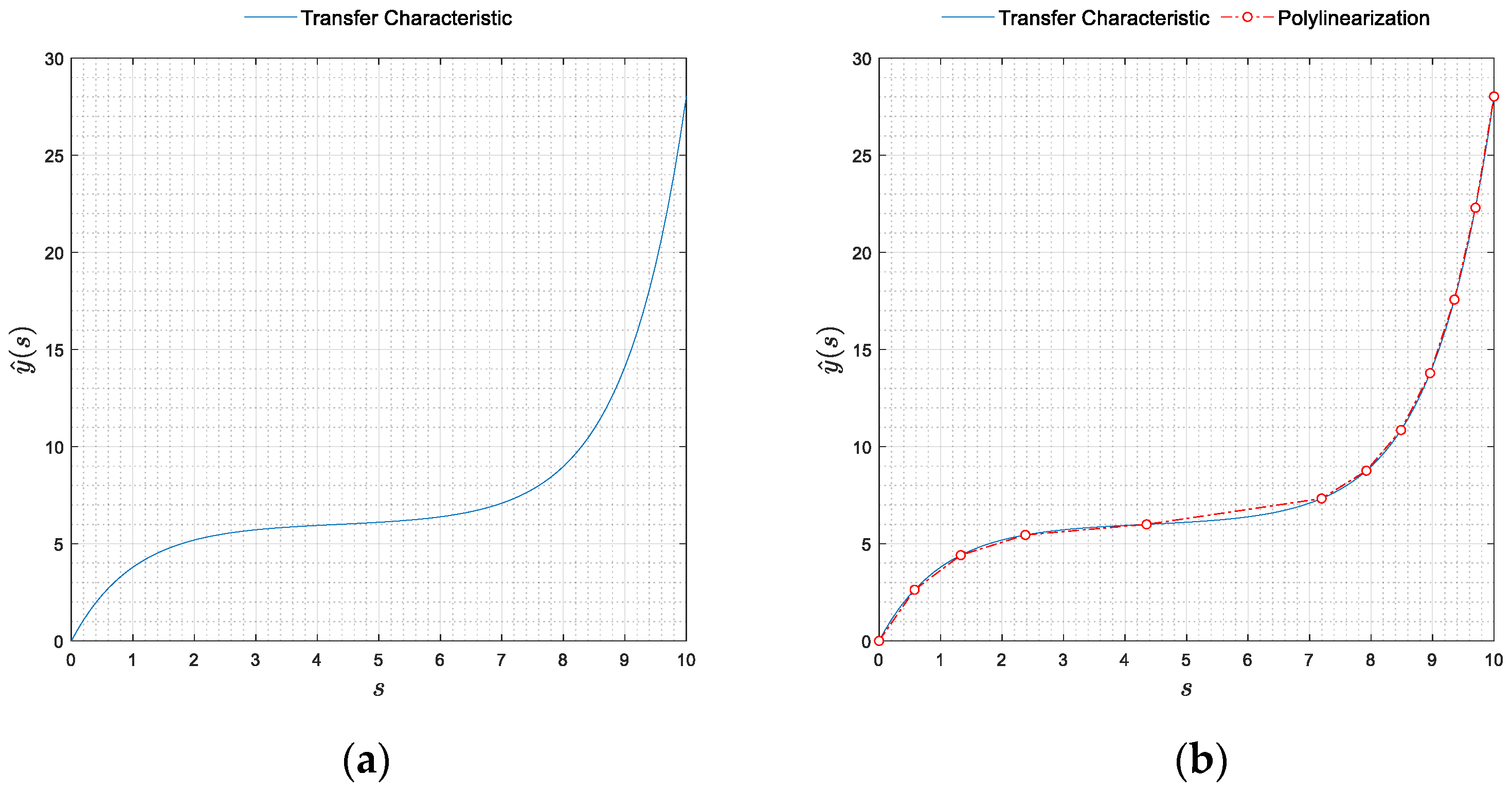
The purpose of this paper is to explain how non-self-intersecting planar curves of finite length can be optimally polylinearized by connecting certain points on them through straight line segments (Figure 1).
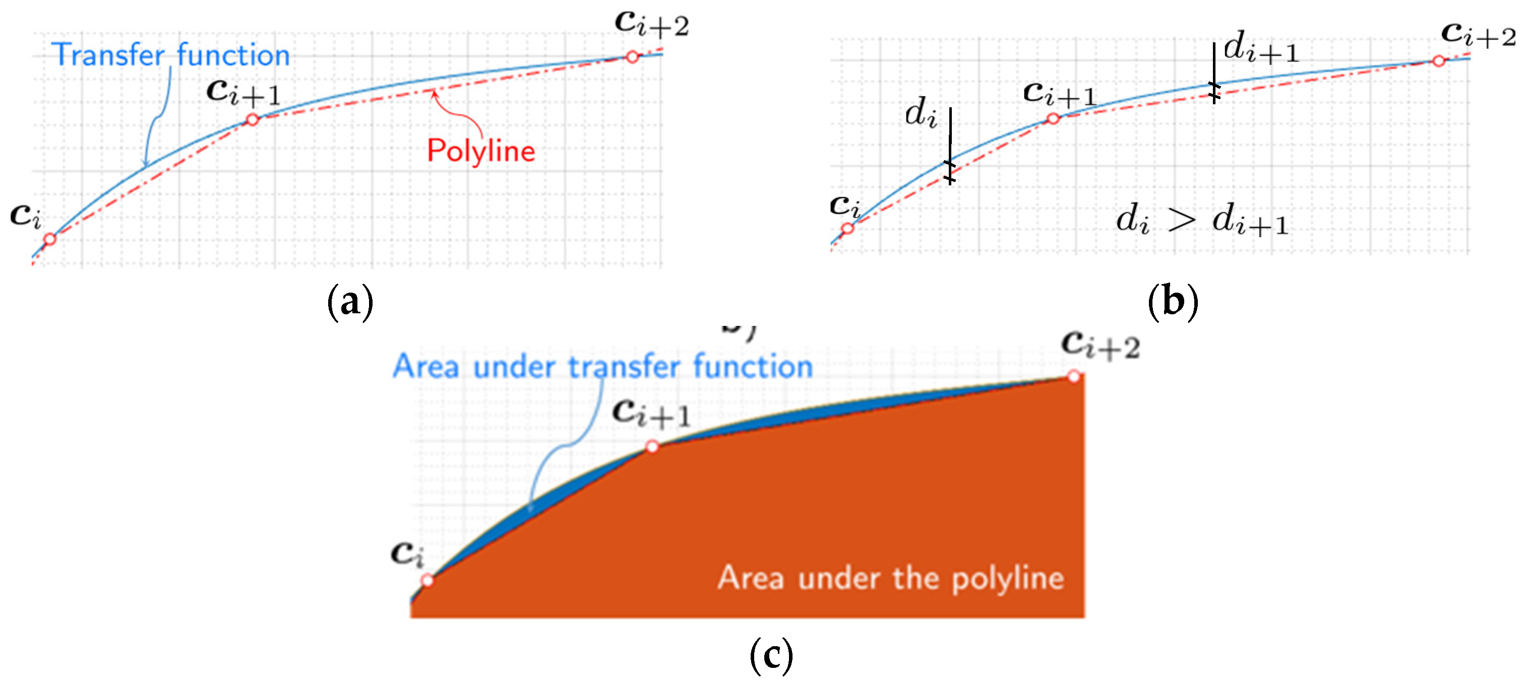
It will be shown below that this problem can be solved as a series of distance/area minimization problems in which the same problem is solved repeatedly, namely, for a fixed pair of points (vertices) and on the curve (Figure 2a), to determine the vertices , so that the polyline (in red) connecting , and is controllably far from the curve.
Of crucial importance here is the choice of the measure of controllable remoteness between a polyline and a curve. The remoteness between two such objects can be estimated in different ways: for example, it can be calculated for each line segment separately, and then, the polyline can be considered to be as far away from the curve as its furthest line segment (Figure 2b). Alternatively, remoteness can be measured in terms of the areas (energies) under the polyline and the curve. The smaller the area values, the closer the curve to the polyline (Figure 2c).
2. Materials and Methods
The approximation of given sensor transfer functions using polylines that is called in this study as polylinearization rests upon three central concepts: the curve segment, the (poly)line segment, and the measure of the remoteness between them. While the curve segment is a differential geometric concept, the polyline segment arises from a much more mundane issue: the need to approximate “in the best possible way” the curve segment by a compact straight line. Conceptually, the process of polylinearization of a given sensor characteristic consists of three algebraic stages. The first (not a subject of the present study) is the representation of the sensor transfer function, i.e., the derivation of its algebraic equations from the physical principles. The second stage is the quantification of the remoteness between the curve and each of its approximating polyline segments. Finally, the third, and in many ways the most important one, is how to construct the polyline best fitting the entire curve, based on the measurement of the remoteness between the curve and the line segments building that polyline.
In this context, this section is an introduction to the instrumentation which will be later used with the following key notions and procedures covered:
- Rectifiable simple curve; curve segment and its approximating (poly)line segment.
- Measuring the remoteness between a curve segment and the corresponding line segment.
- Measuring the remoteness between the curve and the entire polyline.
- Fitting a polyline to a curve by solving a proximity-controlled area-minimization problem for the vertices of the polyline.
Adhering to the above, we organize the text of this section as follows:
- First, we introduce the concepts of a simple rectifiable curve and a curve segment between any two distinct points (also called nodes) on it.
- Second, we characterize in the parametric form the polyline segment between the same two points and introduce the measure of its remoteness from the curve.
- Third, an open chain of connected line segments (polyline, broken-line graph) is constructed, whose proximity to the curve is further evaluated using appropriate distance and area measures. These are nothing but measures of remoteness that non-smoothly tend to become zero as the polyline approaches the curve.
- Finally, we formulate the area-minimization problem with a constraint expressed in terms of a particular remoteness measure; its solution, within the margin of the user-specified tolerance, provides us with the controllable polylinearization of the curve.
At the end of this section, the details of a concrete application of the above general scheme to the practical problem of polylinearization of plane curves are discussed. Here, instead of solving analytically the constrained minimization problem—which was an active topic of research in the 1980s—its (stable and consistent) discrete approximation is solved [26].
2.1. Linearization and Polylinearization Costs
The position (point) in space is indicated by bold lowercase italic letters, such as , etc.
Let us start with the concepts of curve and curve segment: also, given the subset and the natural number, . For , we call the vector-valued map,
a parametrized curve immersed in and write for the points on the curve. A curve, is called simple if it does not intersect itself, and rectifiable if it has a finite length. Furthermore, if is rectifiable, then it is at least of class and hence regular. In the following equations, we deal with simple, rectifiable curves. Let us next set and focus on a particular segment with . The image,
is called the curve segment, starting at and ending at . Let us next clarify what we mean by a line segment attached to a curve segment . For this purpose, we introduce the affine map,
with domain and image . Clearly at , , and at we have .
The line segment, , attached to at and is defined by,
where
How close are and to each other on ? To estimate their proximity, we introduce the measure,
and refer to it as the linearization cost on . In this expression, the -norm, of the difference, is,
with , for .
The notion of linearization cost—essentially localized in —allows easy extension to the entire domain . Accordingly, let be an ascendant partition of , furnished by the nodes , such that for . We call mesh,
the union of subdomains, , i.e., the union of bounded, closed sets, with a nonempty interior. Extending the concept of linearization cost from a single line to a polyline, we introduce the -norm,
on , which shall be referred to in the following sections as the polylinearization cost. Here,
In other words, is the polyline on , consisting of an open chain of line segments, , with the end of each previous segment serving as the beginning of the next.
Considering further the question of the existence of optimal polylinearization, let us first focus on the case of fixed (and hence ). To answer that question, we begin with the observation,
and notice that,
with called the characteristic size of the mesh. On the other hand, the inequality,
implies the estimate,
Hence, the area error is constrained to lie between the following two bounds:
expressed in terms of the polylinearization cost the fixed number of line segments and the characteristic mesh size . Since the curve is simple and rectifiable, this inequality mathematically expresses the two conditions for the existence of an optimal polylinearization:
- (a)
- For a fixed domain there exists such that and the total area error attain their minima.
- (b)
- For a fixed domain there exists such that and the total area error attain their minima.
Regarding (a), an increase in decreases and which in turn, due to the above inequality, implies a decrease in the total area error Analogously, for (b), a decrease in increases and decreases which in turn implies a decrease in the total area error
Therefore, among all admissible nodal locations, , and their associated meshes, there exists at least one node, designated by , which minimizes the polylinearization cost and consequently reduces the total area error. Let us next designate the mesh associated with this partitioning by , and note that if minimizes it will be also the minimizer of the squared polylinearization cost,
which constitutes a quadratic objective function in the nonlinear problem for the optimal polylinearization of rectifiable, planar curves, formulated in the next section. Furthermore, for the range of the total area error, we now have the estimate,
Alternatively, let and be the partition and the associated mesh minimizing the total squared area error,
In general, , and hence, . Furthermore, for the range of the associated polylinearization cost, we analogously have the estimate,
In other words, whichever error we choose to minimize, the other one will be minimized too.
2.2. Remoteness Measures
If is fixed, we will not get controllably close to the polyline by node reallocation alone, as we also need a mechanism to introduce (“inject”) more nodes where it is most necessary. For that to happen, we need one more concept, or more precisely, an -dependent, generalized measure of distance, which we call remoteness measure. Why introduce yet another measure? The reason is primarily epistemological. The optimal polylinearization of a curve consists of two sub-problems: the first is related to “injecting” nodes where they are needed, and the second is related to reallocating these nodes to the positions where they are needed. The latter of these problems has already been addressed. Below, we discuss the former.
Intuitively, an object is as close to another object as its farthest parts are. When the objects are a curve and a polyline, it is natural to ask whether there is a way to estimate how close the farthest segments of the curve and polyline are to each other. The answer to this question is affirmative, and below, we present (with its purpose and merits) a quantitative measure of the distance between a curve and a polyline based on the largest distance between their building components. As it will also become clear, the remoteness is an upper bound on , and depends on the number of nodes, . The latter is crucial as it provides us with the tool to directly influence by modifying its upper bound, or equivalently, by modifying . Furthermore, since the remoteness operates on the line segments furthest from the curve, it will also serve as an identifier of these in which it is feasible to “inject” more nodes.
Using the remoteness measure of order , associated with the mesh , we will understand the limit,
and shall be interested in calculating it for two particular choices of , corresponding to the following:
- -
- The surface remoteness, determined for , as the least upper bound,
- -
- The gap, determined for , and calculated as the largest distance,
For the mesh path in Figure 3, the surface remoteness is
Alternatively, the gap satisfies
However, whatever the choice of , the behavior of either or is always the same, namely, the smaller the remoteness measure for a given mesh , the closer is to . Locally, Euclidean manifolds, to which our rectifiable simple curves belong, are more polylinearizable using finer meshes. In the following considerations, we justify this intuitive understanding as deductively correct and show that the remoteness measures (objects inversely proportional to the number of nodes ) provide upper bounds on (an object dependent on node locations). Increasing will decrease the remoteness between and . In turn, since the remoteness is an upper bound on , by increasing we will further reduce the cost of polylinearization. Let us show this for . Analogous argumentation can be followed for . From the previous section, the following can be recalled,
but
and hence,
Since tends to at a rate proportional to and , therefore, it follows that tends to 0 at a rate proportional to , and hence, increasing decreases as well, which was necessary to show.
2.3. Optimal Polylinearization of Curves
From all possible meshes , we are interested in calculating the one, say , which minimizes the squared polylinearization cost and decreases , below certain user-defined, tolerance, . Such an objective is therefore twofold: on the one hand, it is related to computing the optimal node locations (topology) in , and on the other hand, it is related to determining the optimal number of nodes, in . A possible formulation of the problem targeting this objective is as follows:
Given on and the initial mesh , determine the optimal mesh by solving the minimization problem,
subject to the remoteness control, , with
for or .
Notes:
- (a)
- This problem will be denoted as the optimal polylinearization.
- (b)
- Control over the nodal locations is enforced by an essential minimization problem for the polylinearization cost, while control over the number of nodes is achieved through the corresponding remoteness measure.
- (c)
- The minimization problem is quadratic, while the remoteness control is not, defined by the corresponding -norm, in which is not equal to . Although qualitatively the remoteness measures behave in the same way—the larger the measure, the more distant the polyline and the curve—quantitatively they differ. Thus, different choices for will result in different optimal solutions .
- (d)
- Therefore, we propose the polyline to be always calculated using the minimization of polylinearization cost but to interpret particular solutions as optimal only in the context of the imposed remoteness measure.
- (e)
- The constrained minimization problem allows for vectorial interpretation, because which corresponds to is a vector, whose cardinality and nodal locations, , are its solutions as well.
There are cases where solving the vector minimization problem from the previous section can be effectively reduced to solving a sequence of scalar minimization problems. In this subsection, we consider such a situation—the polylinearization of rectifiable planar curves. At the onset, let us fix the origin and introduce the canonical basis in . Let
be the equation of the curve for . Let us next set, and , with known. For naturally parametrized planar curves alike, the minimization problem from the previous section reads as follows.
Given on and the initial mesh , determine the optimal mesh by solving the optimization problem of planar polylinearization,
with constraint
In what follows, we will be interested in calculating for .
The separate contributions to this minimization problem are as follows:
- -
- Typical, planar line segment, , on , has the representation:
- -
- The linearization cost of , denoted by , is
- -
- The polylinearization cost, , is
and the surface remoteness is .
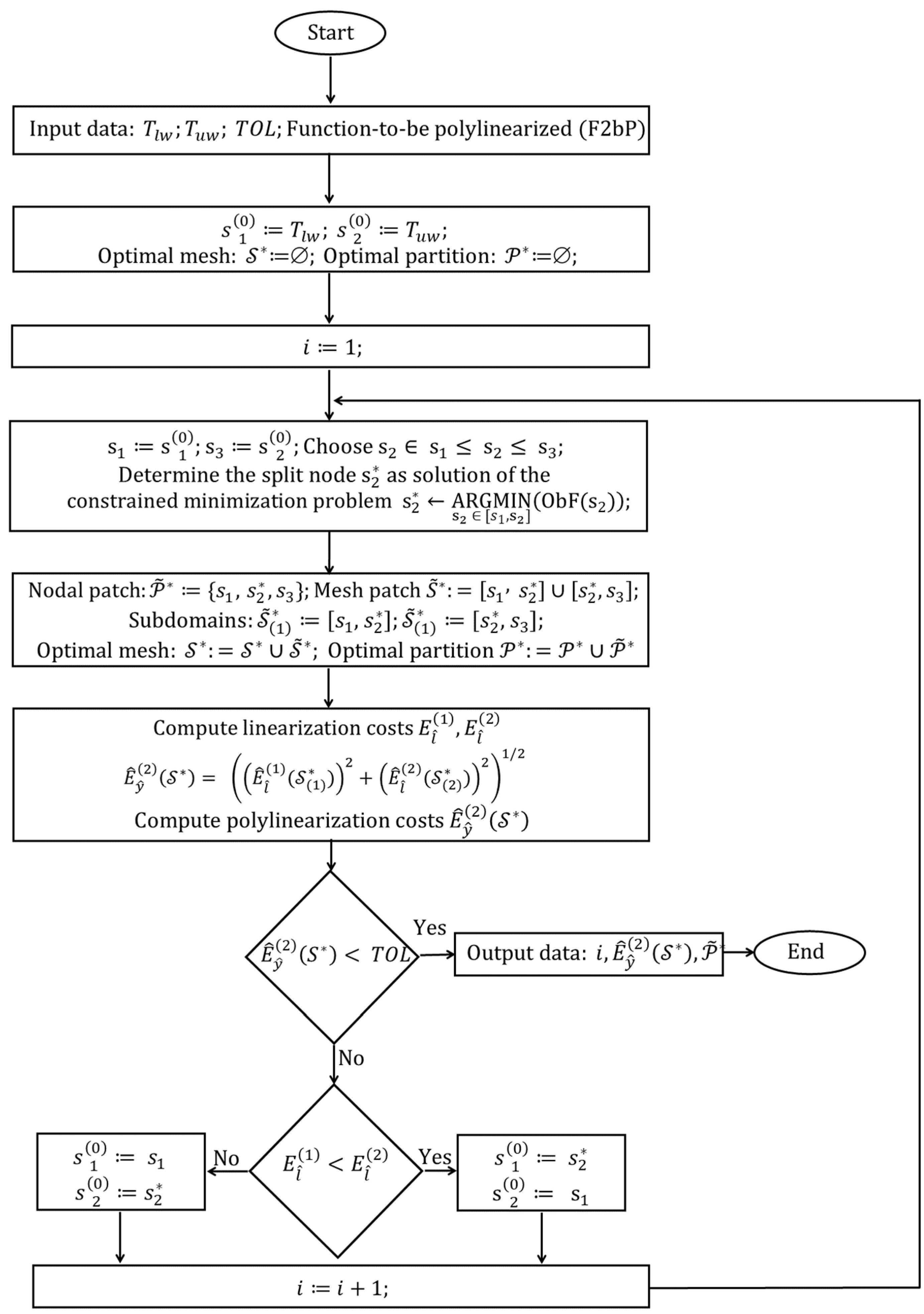
Instead of using the Lagrangian multiplier to enforce the proximity control on we will approach the solution in a slightly different way. Let us first initialize the optimal partition and the optimal mesh using the following setting: , . The initial partition, , with and is known and fixed. Let us next consider a nodal patch, , obtained from by adding a node, , of a yet unknown location, but between and , so that , and . With the mesh patch, , instilled by , the vector minimization problem with the objective function, , transforms into a scalar minimization problem for with objective function, , and constraints, .
Let us designate the solution of this minimization problem by and the corresponding optimal nodal patch by . The optimal partition, , is next updated with this patch so that, . The split node, , now divides into two subdomains, i.e., and , so that the current mesh instilled by is analogously calculated through the update , and consists of . Furthermore, once determined, the mesh allows us to compute and compare it with TOL. If , our task is complete; otherwise, if , we need to add more nodes between and , and compute their location by constrained minimization.
The following question still exists, i.e., in which of the subdomains or should new split node(s) be added? On the one hand, we do not want to add too many nodes, and on the other hand, we do not want to add too few. The former requires more storage space, while the latter requires more computational time. Let us agree to add no more than one node per interval and focus on how to select the appropriate interval. The reliable selection criterion is provided by the largest surface remoteness, determined over the current set of subdomains in the mesh, i.e., the candidate subdomains for splitting are those whose surface remoteness is the largest, or
In our particular case, splits into two subdomains with the following surface remotenesses:
Assume for the sake of clarity that the whose is the largest corresponds to , and is overwritten by and .
Analogous to what we did before, we constructed from by allocating a node, between and so that for , we again have , , and . Let us consider as unknown and determine it by the constrained minimization of , thus updating the optimal nodal patch,
, and the mesh patch,
Further, with and already updated, we update the optimal partition and the optimal mesh, , , so that
Once we have , we again compute and compare it with . If we stop the computation; otherwise, we repeat again the surface-remoteness-based approach for the selection of the next candidate subdomain for splitting. In the above procedure, it is easy to notice the following: first, the sequence of points is generated as a solution to the corresponding sequence of constrained minimization problems for the unknown , and second, each minimization problem in this sequence is solved over a subdomain with fixed ends.
The main steps of the developed algorithm are shown in Figure 4.
3. Results
The polylinearization of typical nonlinear sensor transfer functions concerning and norm is discussed below:
- -
- -
- -
- -
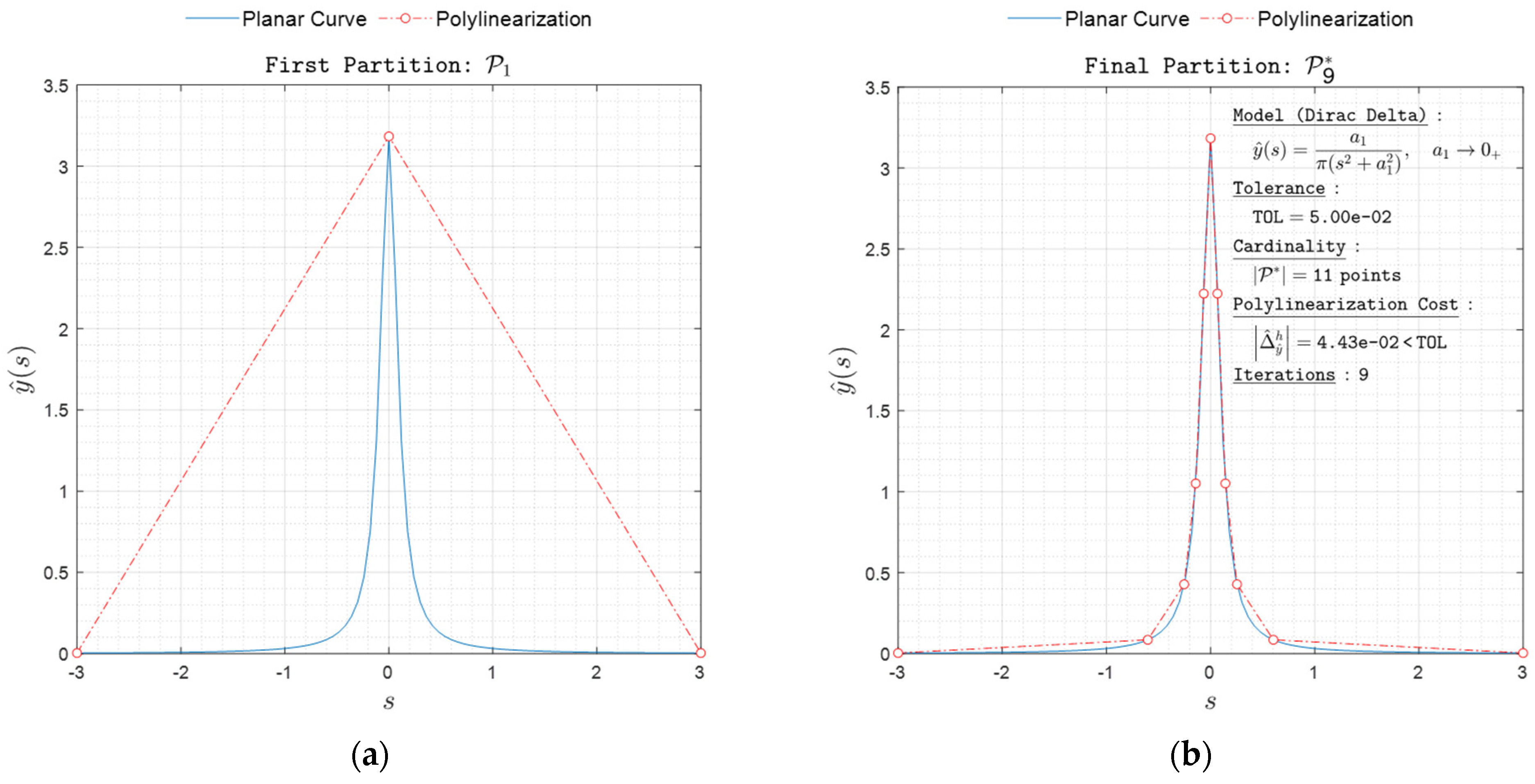
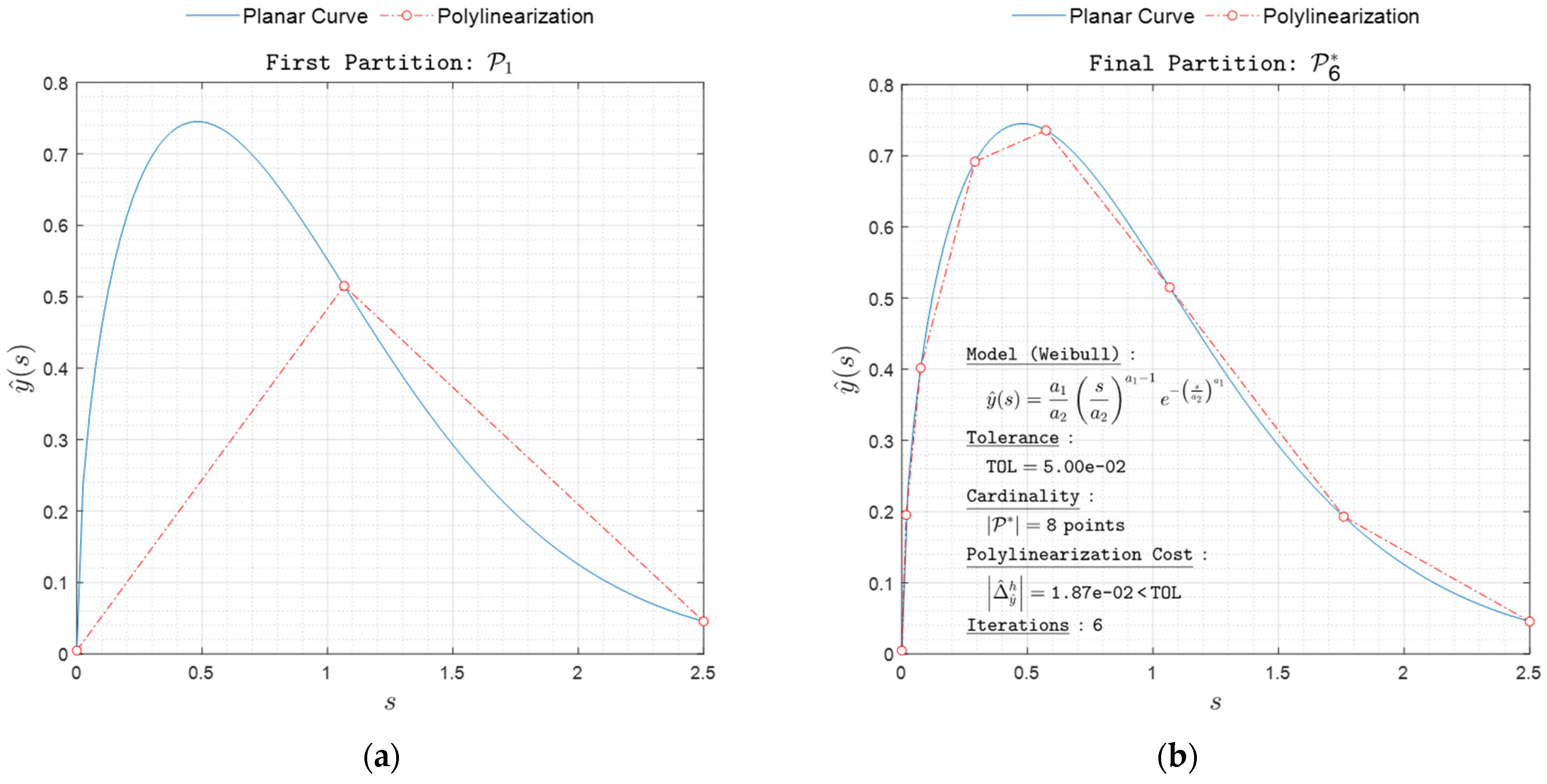
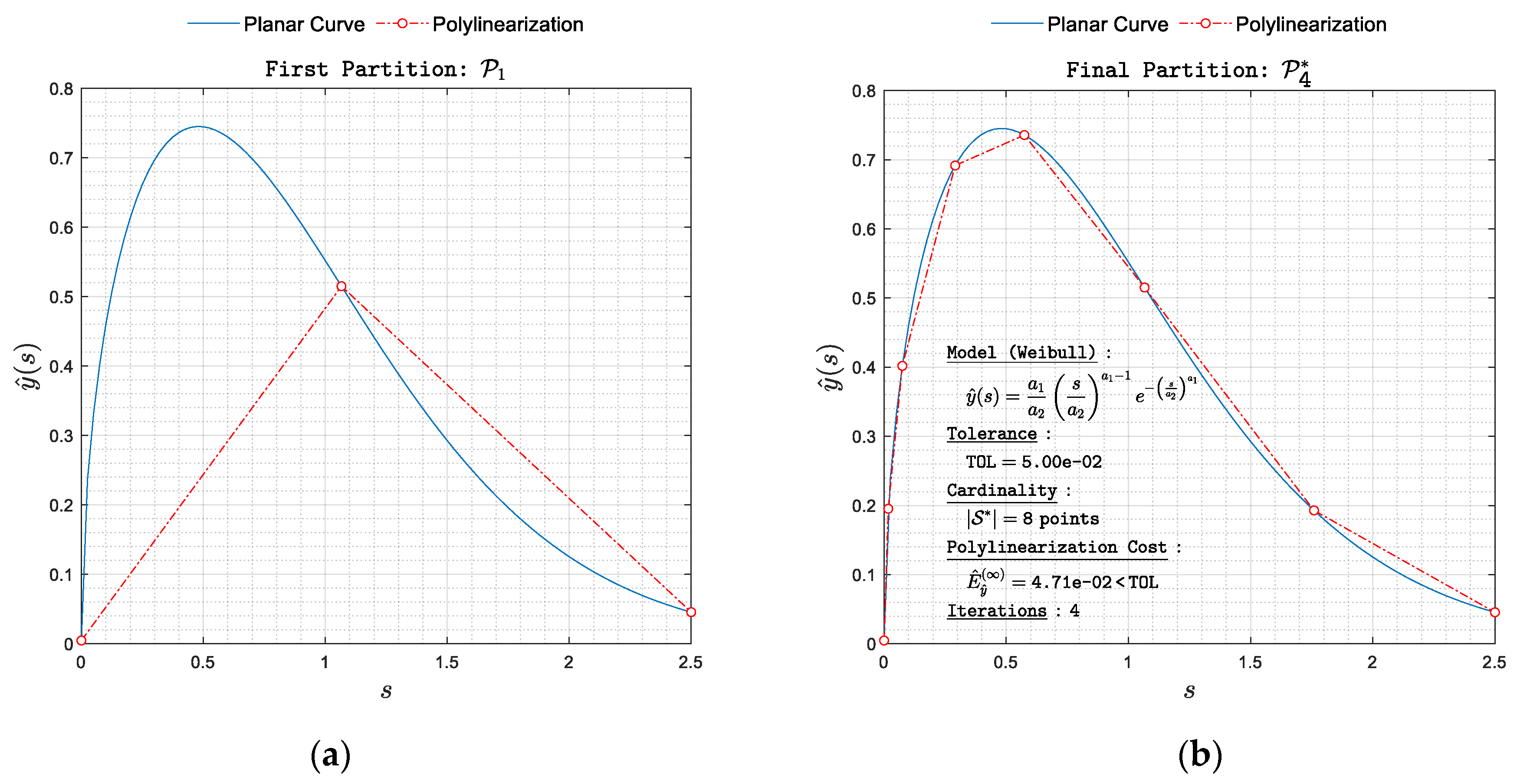
Along with the polylinearization of sensor transfer functions, the polylinearization of functions and distributions commonly used in scientific research is considered. Examples given here are as follows:
The main results of the study can be summarized as follows:
- A numerical polylinearization approach is proposed for both types of rectifiable sensor characteristics: either concave or convex.
- The approach is sufficiently general and allows applications to both two-dimensional and three-dimensional characteristics.
- The problem of optimal vertex allocation of the approximating polyline is discretized using a second-order accurate integration rule and then solved numerically. Higher-order integration rules are also allowed and will not change the algorithmic solution.
- The applicability of the approach is illustrated by several well-known sensory characteristics.
4. Conclusions
Generally, the term “polylinearization” suggests a mathematical process used to model and compensate for nonlinear behavior in sensors or devices. When sensors or IoT devices produce nonlinear responses, it can be challenging to obtain accurate measurements and data. Polylinearization techniques involve the application of mathematical functions to transform the sensor’s output into a linear relationship with the input, thus significantly improving the measurement accuracy.
This paper discusses the optimal polylinearization of non-self-intersecting planar curves of finite length by connecting certain points on them through straight line segments. The problem can be solved as a series of constrained distance/area minimization problems, where the same issue is resolved repeatedly. The choice of the measure of controllable remoteness between a polyline and a curve is crucial, as it can be estimated in different ways. The polylinearization process consists of three algebraic stages: representing the sensor transfer function, quantifying the remoteness between the curve and its approximating polyline segments, and constructing the polyline best fitting the entire curve based on the measurement of the remoteness between the curve and the line segments building that polyline. The study introduces the concepts of a simple rectifiable curve and a curve segment between any two distinct points, characterizes the polyline segment in parametric form, builds a polyline, and estimates its proximity to the curve in terms of distance- and area-related measures. The area-minimization problem is solved with a constraint expressed in terms of a particular remoteness measure, providing the controllable polylinearization of the curve.
This study discusses a new concept of linearization and polylinearization costs in the context of curves and curve segments. It begins with the definition of a vector-valued map, a parametrized curve, and its properties. Line segments attached to a curve segment are defined by the affine map with domain and image. The linearization cost on a line segment is used to estimate their proximity. The concept of linearization cost extends to the entire domain, allowing easy extension to the union of subdomains. The polylinearization cost is the linearization cost from a single line to a polyline, consisting of an open chain of line segments. The text also discusses the existence of an optimal polylinearization, focusing on fixed domains and the characteristic mesh size. Inequality expresses the conditions for an optimal polylinearization, stating that for a fixed domain, the total area error attains its minima.
Author Contributions
Conceptualization, M.B.M. and S.D.; methodology, S.D. and M.B.M., software, S.D.; investigation, S.D.; resources, S.D. and M.B.M.; writing—original draft preparation, M.B.M. and S.D.; writing—review and editing, M.B.M.; visualization, S.D. All authors have read and agreed to the published version of the manuscript.
Funding
This research is supported by the Bulgarian National Science Fund within the framework of the “Exploration of the application of statistics and machine learning in electronics” project under contract number KП-06-H42/1.
Data Availability Statement
Data are contained within the article.
Acknowledgments
The authors would like to thank the Research and Development Sector at the Technical University of Sofia for the financial support.
Conflicts of Interest
The authors declare no conflicts of interest.
Nomenclature
| natural numbers | |
| integers | |
| real numbers | |
| set of n-tuples of real numbers | |
| Euclidian 3-D point space | |
| the two-dimensional subspace of | |
| position vector (lower-case, boldface, italic symbols) | |
| length of a vector , | |
| function rule | |
| value of a function | |
| partial derivatives of in | |
| set of elements | |
| number of elements (cardinality) in a set | |
| linear segment | |
| length of a linear segment |
References
- Attari, M. Methods for linearization of non-linear sensors. Proc. CMMNI-4 1993, 1, 344–350. [Google Scholar]
- Pereira, J.M.D.; Postolache, O.; Girao, P.M.B.S. PDF-Based Progressive Polynomial Calibration Method for Smart Sensors Linearization. IEEE Trans. Instrum. Meas. 2009, 58, 3245–3252. [Google Scholar] [CrossRef]
- Erdem, H. Implementation of software-based sensor linearization algorithms on low-cost microcontrollers. ISA Trans. 2010, 49, 552–558. [Google Scholar] [CrossRef] [PubMed]
- Johnson, C. Process Control Instrumentation Technology, 8th ed.; Pearson Education Limited: London, UK, 2013. [Google Scholar]
- Lundström, H.; Mattsson, M. Modified Thermocouple Sensor and External Reference Junction Enhance Accuracy in Indoor Air Temperature Measurements. Sensors 2021, 21, 6577. [Google Scholar] [CrossRef] [PubMed]
- Marinov, M.; Dimitrov, S.; Djamiykov, T.; Dontscheva, M. An Adaptive Approach for Linearization of Temperature Sensor Characteristics. In Proceedings of the 27th International Spring Seminar on Electronics Technology, ISSE 2004, Bankya, Bulgaria, 13–16 May 2004. [Google Scholar]
- Šturcel, J.; Kamenský, M. Function approximation and digital linearization in sensor systems. AT&P J. 2006, 1, 13–17. [Google Scholar]
- Flammini, A.; Marioli, D.; Taroni, A. Transducer output signal processing using an optimal look-up table in mi-crocontroller-based systems. Electron. Lett. 2010, 33, 552–558. [Google Scholar]
- Islam, T.; Mukhopadhyay, S. Linearization of the sensors characteristics: A review. Int. J. Smart Sens. Intell. Syst. 2019, 12, 1–21. [Google Scholar] [CrossRef]
- van der Horn, G.; Huijsing, J. Integrated Smart Sensors: Design and Calibration; Springer: New York, NY, USA, 2012. [Google Scholar]
- Berahmand, K.; Mohammadi, M.; Saberi-Movahed, F.; Li, Y.; Xu, Y. Graph Regularized Nonnegative Matrix Factorization for Community Detection in Attributed Networks. IEEE Trans. Netw. Sci. Eng. 2023, 10, 372–385. [Google Scholar] [CrossRef]
- Nasiri, E.; Berahmand, K.; Li, Y. Robust graph regularization nonnegative matrix factorization for link prediction in attributed networks. Multimed. Tools Appl. 2023, 82, 3745–3768. [Google Scholar] [CrossRef]
- Marinov, M.; Nikolov, N.; Dimitrov, S.; Todorov, T.; Stoyanova, Y.; Nikolov, G. Linear Interval Approximation for Smart Sensors and IoT Devices. Sensors 2022, 22, 949. [Google Scholar] [CrossRef] [PubMed]
- Grützmacher, F.; Beichler, B.; Hein, A.; Kirste, T.; Haubelt, C. Time and Memory Efficient Online Piecewise Linear Approximation of Sensor Signals. Sensors 2018, 18, 1672. [Google Scholar] [CrossRef] [PubMed]
- Ouafiq, E.; Saadane, R.; Chehri, A. Data Management and Integration of Low Power Consumption Embedded Devices IoT for Transforming Smart Agriculture into Actionable Knowledge. Agriculture 2022, 12, 329. [Google Scholar] [CrossRef]
- Mitro, N.; Krommyda, M.; Amditis, A. Smart Tags: IoT Sensors for Monitoring the Micro-Climate of Cultural Heritage Monuments. Appl. Sci. 2022, 12, 2315. [Google Scholar] [CrossRef]
- Popivanov, I.; Miller, R.J. Similarity search over time series data using wavelets. In Proceedings of the 18th International Conference on Data Engineering, San Jose, CA, USA, 26 February–1 March 2002. [Google Scholar]
- Rafiei, D. On similarity-based queries for time series data. In Proceedings of the 15th International Conference on Data Engineering, Sydney, Australia, 23–26 March 1999. [Google Scholar]
- Cai, Y.; Ng, R. Indexing spatio-temporal trajectories with Chebyshev polynomials. In Proceedings of the 2004 ACM SIGMOD International Conference on Management of Data, Paris, France, 13–18 June 2004. [Google Scholar]
- Yi, B.; Faloutsos, C. Fast time sequence indexing for arbitrary lp norms. In Proceedings of the 26th International Conference on Very Large Data Bases, Cairo, Egypt, 10–14 September 2000. [Google Scholar]
- Luo, G.; Yi, K.; Cheng, S.; Li, Z.; Fan, W.; He, C.; Mu, Y. Piecewise linear approximation of streaming time-series data with max-error guarantees. In Proceedings of the 2015 IEEE 31st International Conference on Data Engineering (ICDE), Seoul, Republic of Korea, 13–17 April 2015. [Google Scholar]
- Palpanas, T.; Vlachos, M.; Keogh, E.; Gunopulos, D.; Truppel, W. Online amnesic approximation of streaming time series. In Proceedings of the 20th International Conference on Data Engineering, Boston, MA, USA, 2 April 2004. [Google Scholar]
- Chen, Q.; Chen, L.; Lian, X.; Liu, Y.; Yu, J.X. Indexable PLA for efficient similarity search. In Proceedings of the 33rd International Conference on Very Large Data Bases, Vienna, Austria, 23–27 September 2007. [Google Scholar]
- Cameron, S.H. Piece-Wise Linear Approximations; DTIC Document, Technical Report; IIT Research Institute Press: Chicago, IL, USA, 1966. [Google Scholar]
- Marinov, M.; Nikolov, N.; Dimitrov, S.; Ganev, B.; Nikolov, G.; Stoyanova, Y.; Todorov, T.; Kochev, L. Linear Interval Approximation of Sensor Characteristics with Inflection Points. Sensors 2023, 23, 2933. [Google Scholar] [CrossRef] [PubMed]
- Fuchs, E.; Gruber, T.; Nitschke, J.; Sick, B. Online segmentation of time series based on polynomial least-squares approximations. IEEE Trans. Pattern Anal. Mach. Intell. 2010, 32, 2232–2245. [Google Scholar] [CrossRef] [PubMed]
Figure 1.
(a) Smooth sensor transfer function; (b) polylinearization of the sensor transfer function and the approximating polyline, together with its vertices shown in red.
Figure 1.
(a) Smooth sensor transfer function; (b) polylinearization of the sensor transfer function and the approximating polyline, together with its vertices shown in red.

Figure 2.
(a) a polyline through and (b) distance-based remoteness—sensor transfer characteristics and a polyline are as far away from each other as the largest projected distance, ; (c) and area-based remoteness—polyline is as far away from the sensor curve as the area ■ is close to the area ■ (overlapped by ■ and not fully visible).

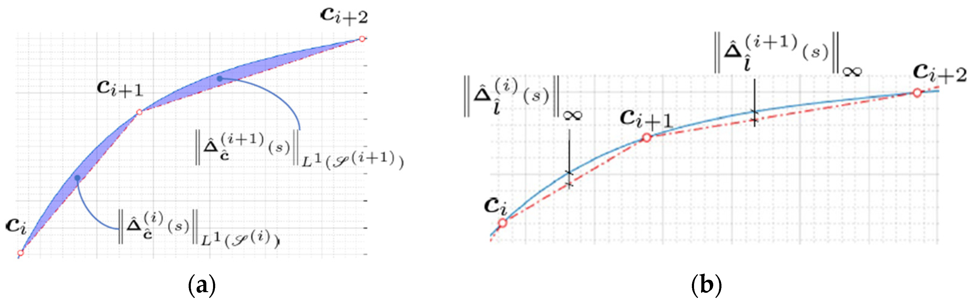
Figure 3.
Illustrations of the concept of remoteness measure for mesh patch : (a) equals the largest of the differences in the areas under the curve segments and their approximating linear segments and (b) equals the largest of the distances between the curve segments and their approximating linear segments.

Figure 4.
Flow chart of the developed algorithm.

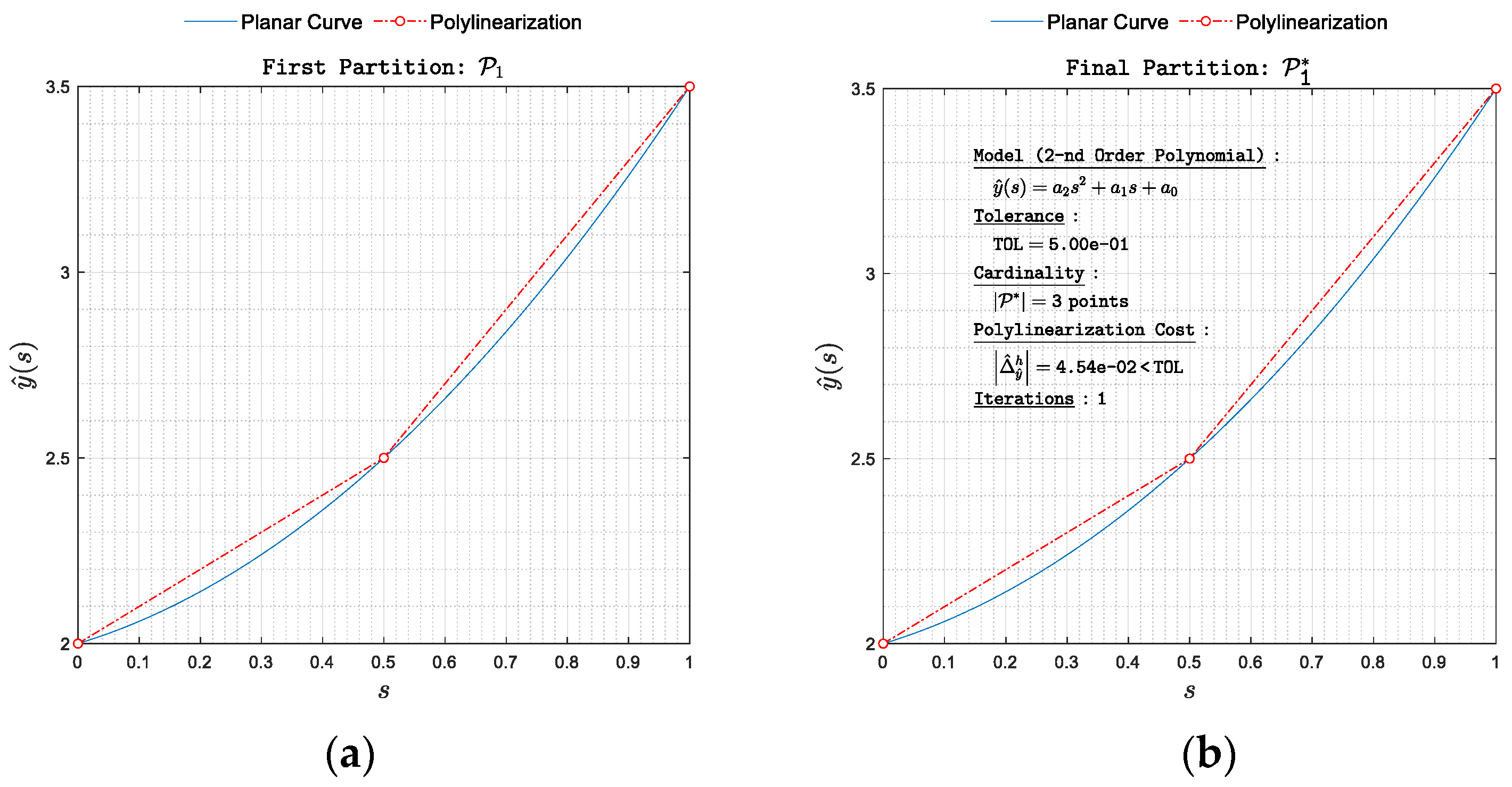
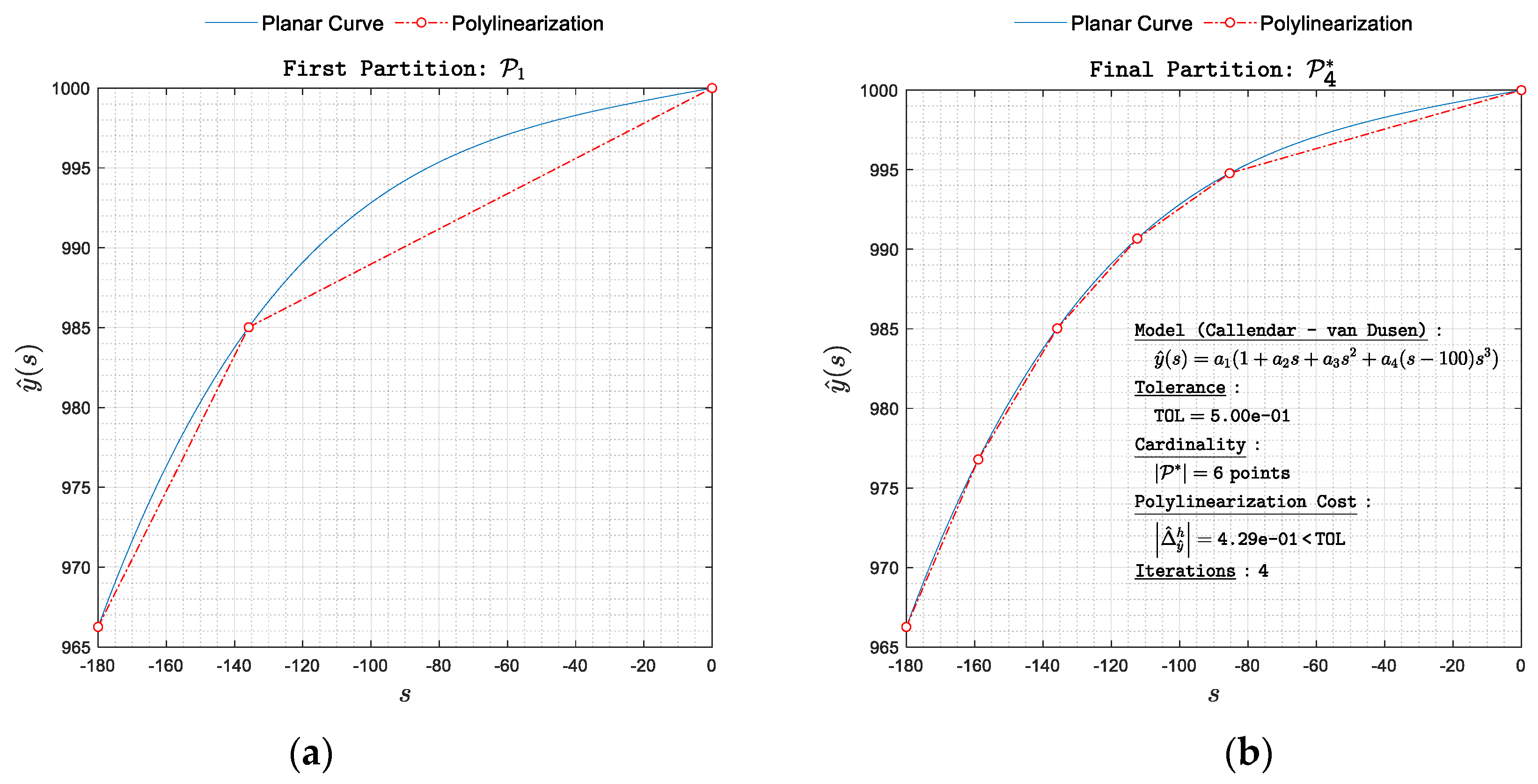
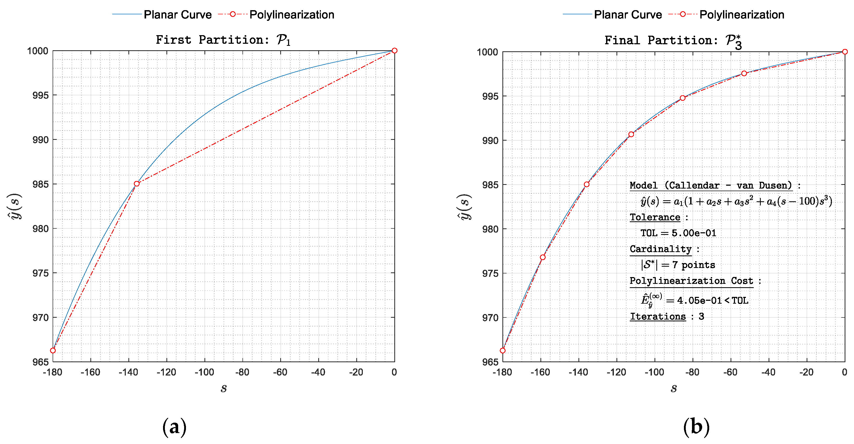
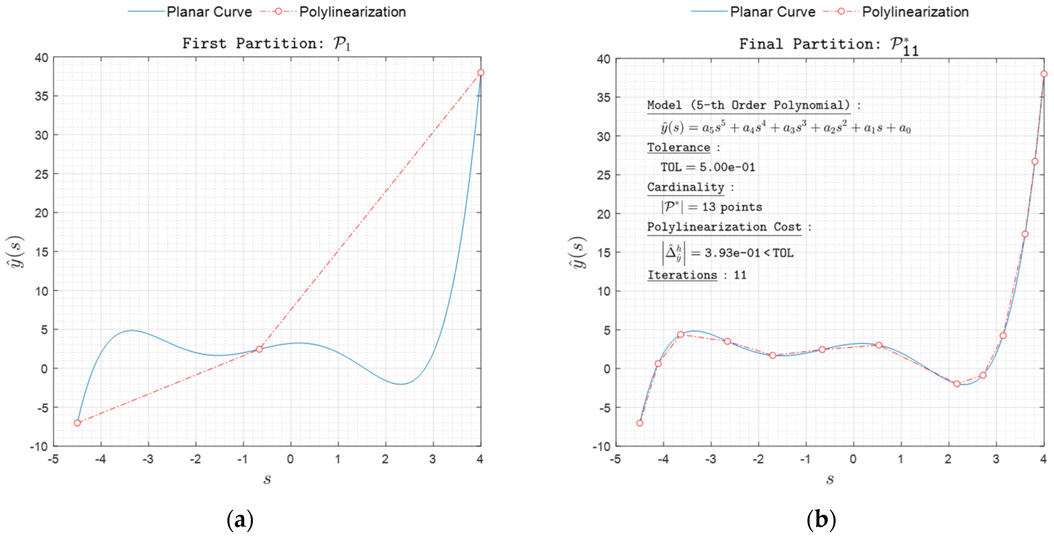
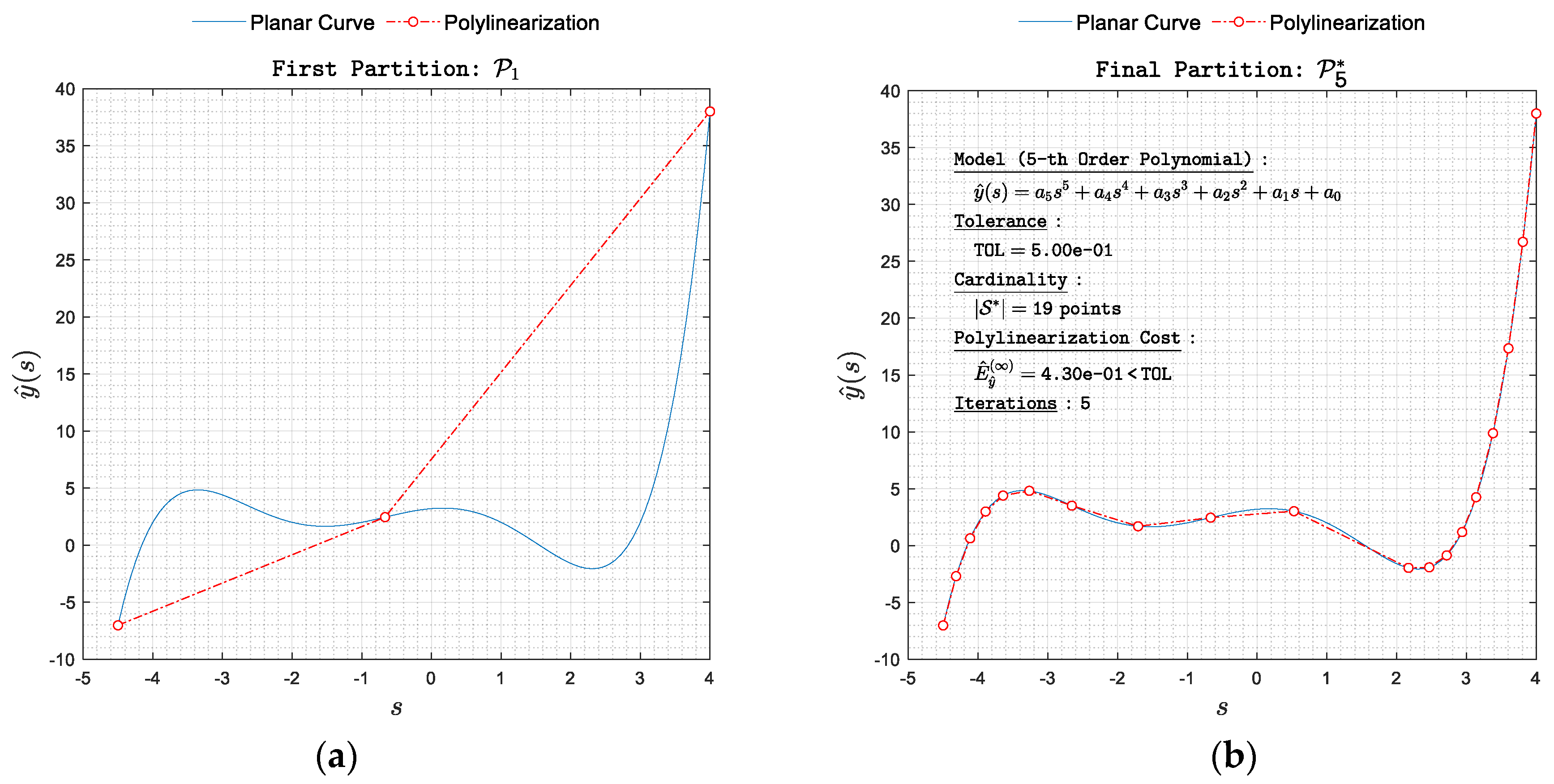
Figure 5.
Polylinearization of with respect to norm. (a) First partition and (b) final partition .

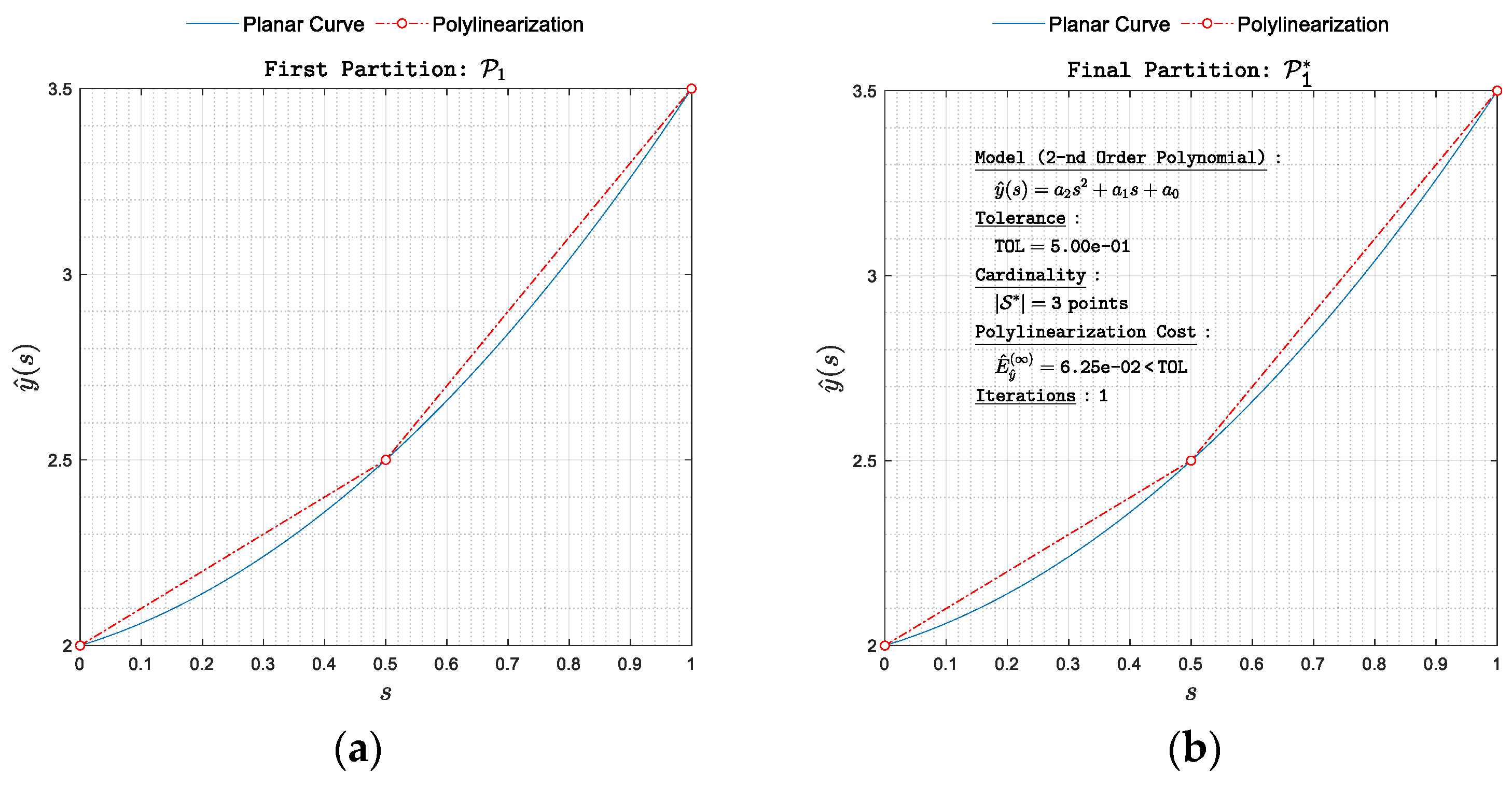
Figure 6.
Polylinearization of with respect to norm. (a) First partition and (b) final partition .

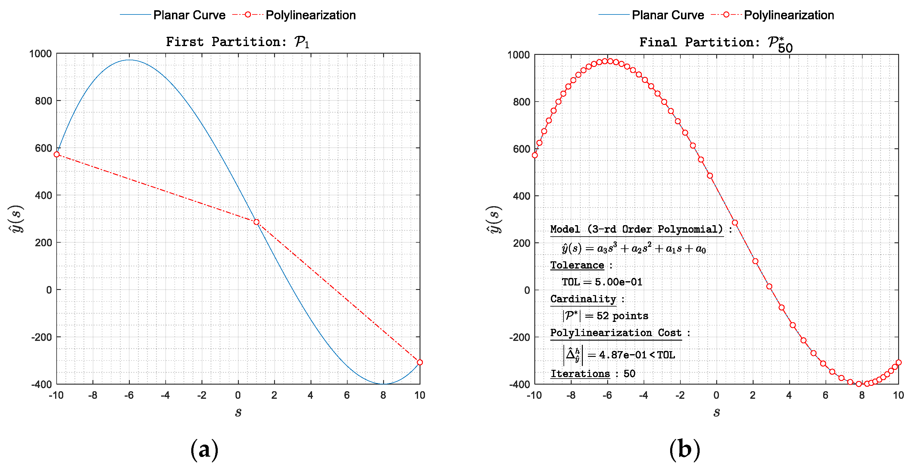
Figure 7.
Polylinearization of with respect to norm. (a) First partition and (b) final partition .

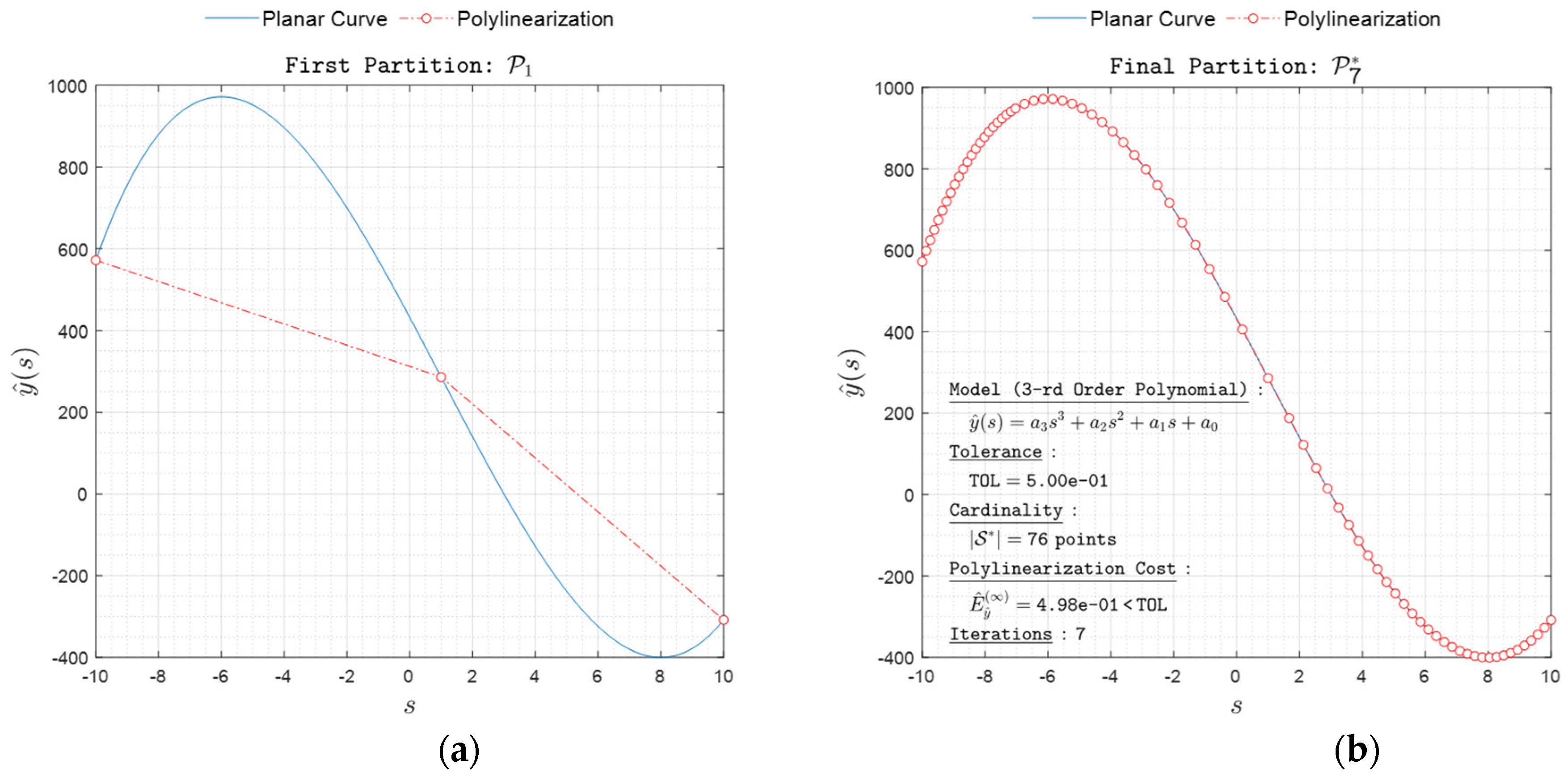
Figure 8.
Polylinearization of with respect to norm. (a) First partition and (b) final partition .

Figure 9.
Polylinearization of with respect to norm. (a) First partition and (b) final partition .

Figure 10.
Polylinearization of with respect to norm. (a) First partition and (b) final partition .

Figure 11.
Polylinearization of with respect to norm. (a) First partition and (b) final partition .

Figure 12.
Polylinearization of with respect to norm. (a) First partition and (b) final partition .

Figure 13.
Polylinearization of with respect to norm. (a) First partition and (b) final partition .

Figure 14.
Polylinearization of with respect to norm. (a) First partition and (b) final partition .

Figure 15.
Polylinearization of with respect to norm. (a) First partition and (b) final partition .

Figure 16.
Polylinearization of with respect to norm. (a) First partition and (b) final partition .

Disclaimer/Publisher’s Note: The statements, opinions and data contained in all publications are solely those of the individual author(s) and contributor(s) and not of MDPI and/or the editor(s). MDPI and/or the editor(s) disclaim responsibility for any injury to people or property resulting from any ideas, methods, instructions or products referred to in the content. |
© 2024 by the authors. Licensee MDPI, Basel, Switzerland. This article is an open access article distributed under the terms and conditions of the Creative Commons Attribution (CC BY) license (https://creativecommons.org/licenses/by/4.0/).
Share and Cite
MDPI and ACS Style
Marinov, M.B.; Dimitrov, S. Generalized Approach to Optimal Polylinearization for Smart Sensors and Internet of Things Devices. Computation 2024, 12, 63. https://doi.org/10.3390/computation12040063
AMA Style
Marinov MB, Dimitrov S. Generalized Approach to Optimal Polylinearization for Smart Sensors and Internet of Things Devices. Computation. 2024; 12(4):63. https://doi.org/10.3390/computation12040063
Chicago/Turabian StyleMarinov, Marin B., and Slav Dimitrov. 2024. "Generalized Approach to Optimal Polylinearization for Smart Sensors and Internet of Things Devices" Computation 12, no. 4: 63. https://doi.org/10.3390/computation12040063
Note that from the first issue of 2016, this journal uses article numbers instead of page numbers. See further details here.