Crop Dominance Mapping with IRS-P6 and MODIS 250-m Time Series Data

 ,
, 

Abstract
:1. Introduction
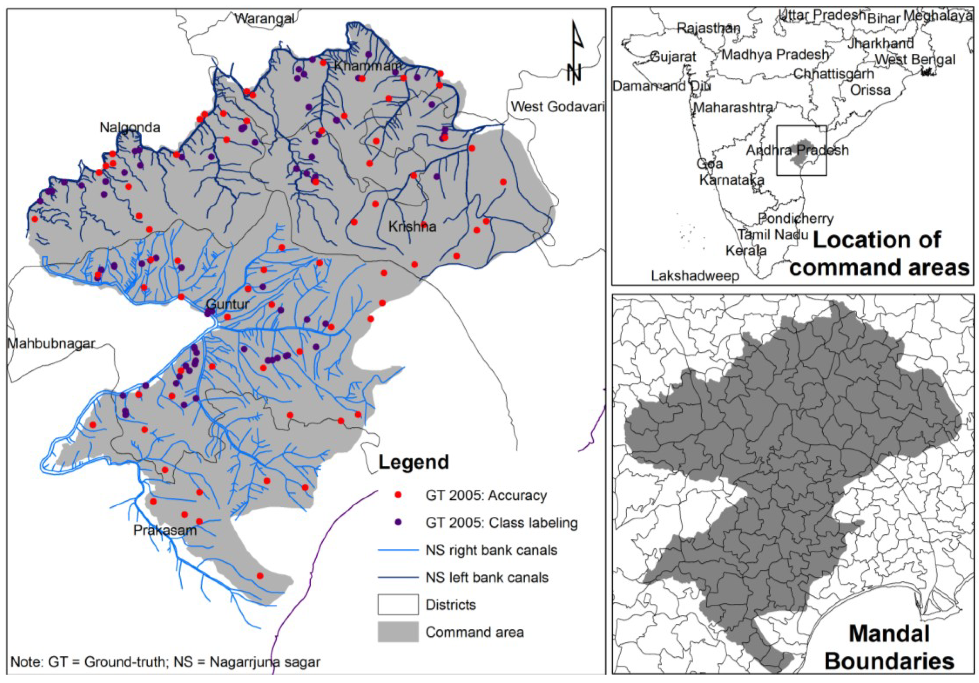
2. Study Area

3. Data and Methods
3.1. IRS-P6 Data
3.2. MODIS 250-m Time Series Data

| Sensor | Spatial(meters) | Bands | Band Range(μm) | Irradiance(W m−2 sr−1 mm−1) | Potential Application |
|---|---|---|---|---|---|
| IRS-P6(5 October 2005, 21 November 2005) | 23.6 | 2 | 0.52–0.59 | 1857.7 | Water bodies and also capable of differentiating soil and rock surfaces from vegetation |
| 3 | 0.62–0.68 | 1556.4 | Sensitive to water turbidity differences | ||
| 4 | 0.77–0.86 | 1082.4 | Sensitive to the strong chlorophyll absorption region and the strong reflectance region for most soils | ||
| 5 | 1.55–1.70 | 239.84 | Operates in the best spectral region to distinguish vegetation varieties and conditions | ||
| MODIS (June 2005 to May 2006) | 250 | 1 | 0.62–0.67 | 1528.2 | Absolute land cover transformation, vegetation chlorophyll |
| 2 | 0.84–0.88 | 974.3 | Cloud amount, vegetation land cover transformation |
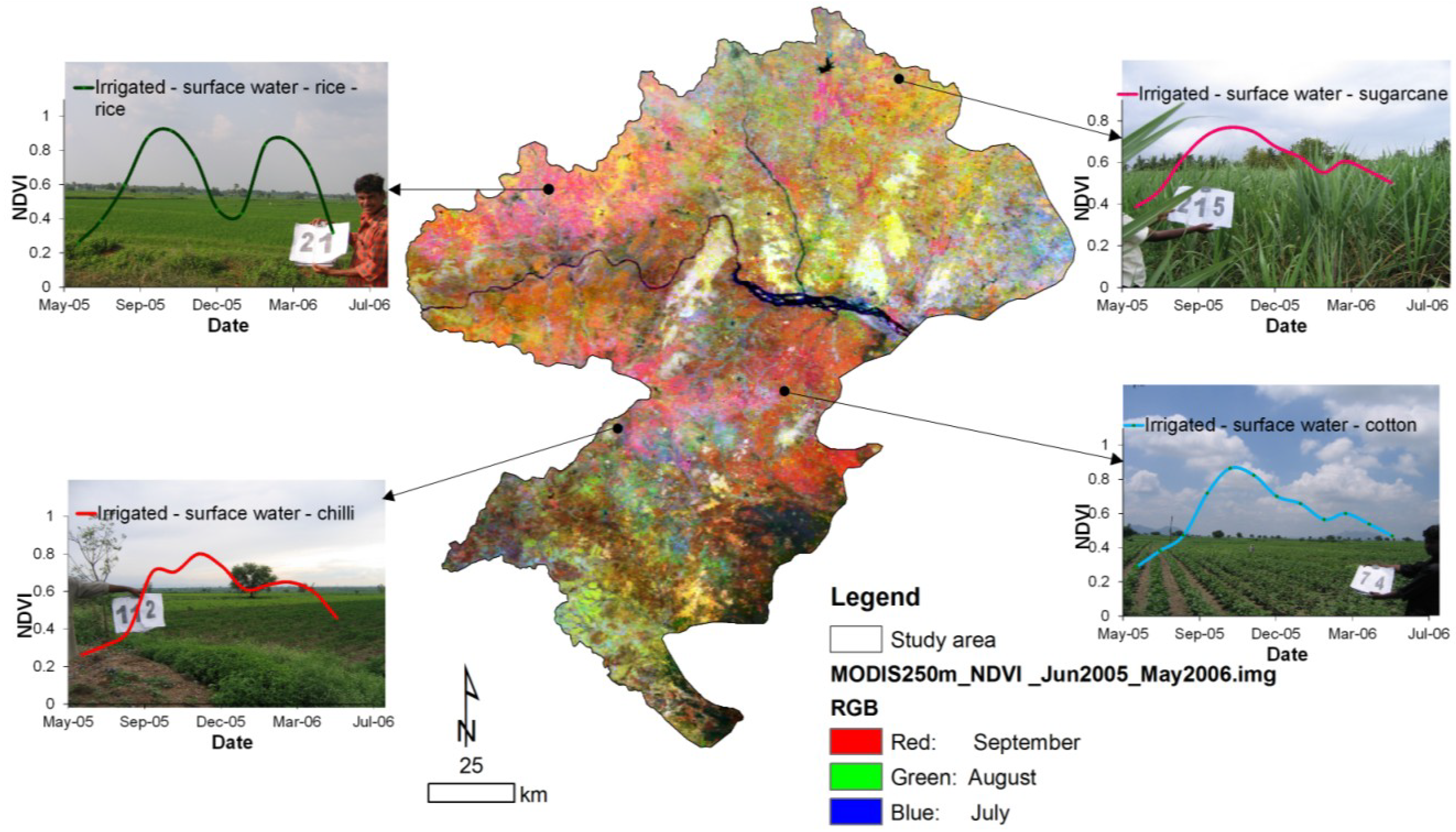
3.3. Ground-Truth Datasets
- Land use land cover (LULC) classes: crop type and other land use and land cover;
- Land cover types (% cover): trees, shrubs, grasses, built-up, water, fallow lands, weeds, different crops, sand, snow, rock and fallow farms;
- Crop types: for Kharif, Rabi and summer seasons;
- Cropping pattern: for Kharif, Rabi and summer seasons;
- Cropping calendar (sowing to harvesting the crop): for Kharif, Rabi and summer seasons;
- Irrigated, rainfed, supplemental irrigation at each location;
- Three hundred forty-four digital photos hot linked at 172 locations.
3.4. Ideal Spectra Creation
3.5. Classification Methods
4. Results and Discussions
4.1. Crop Dominance Classification and Statistics
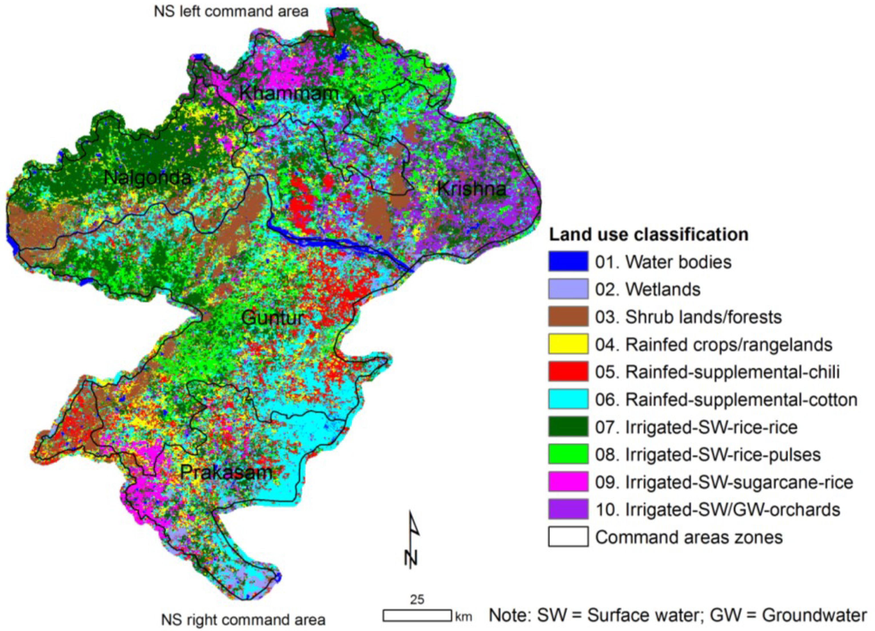
| LULC (No.) | Areas (ha) | % |
|---|---|---|
| 01. Water bodies | 45,632 | 2 |
| 02. Wetlands | 46,833 | 3 |
| 03. Shrub lands/forests | 216,178 | 12 |
| 04. Rainfed crops/rangelands | 158,683 | 9 |
| 05. Rainfed-supplemental-chili | 174,261 | 9 |
| 06. Rainfed-supplemental-cotton dominant chili | 371,803 | 20 |
| 07. Irrigated-SW-rice-rice | 431,992 | 23 |
| 08. Irrigated-SW-rice-pulses | 188,125 | 10 |
| 09. Irrigated-SW-sugarcane-rice | 82,847 | 4 |
| 10. Irrigated-SW/GW-orchards | 141,003 | 8 |
| Total | 1,857,358 | 100 |
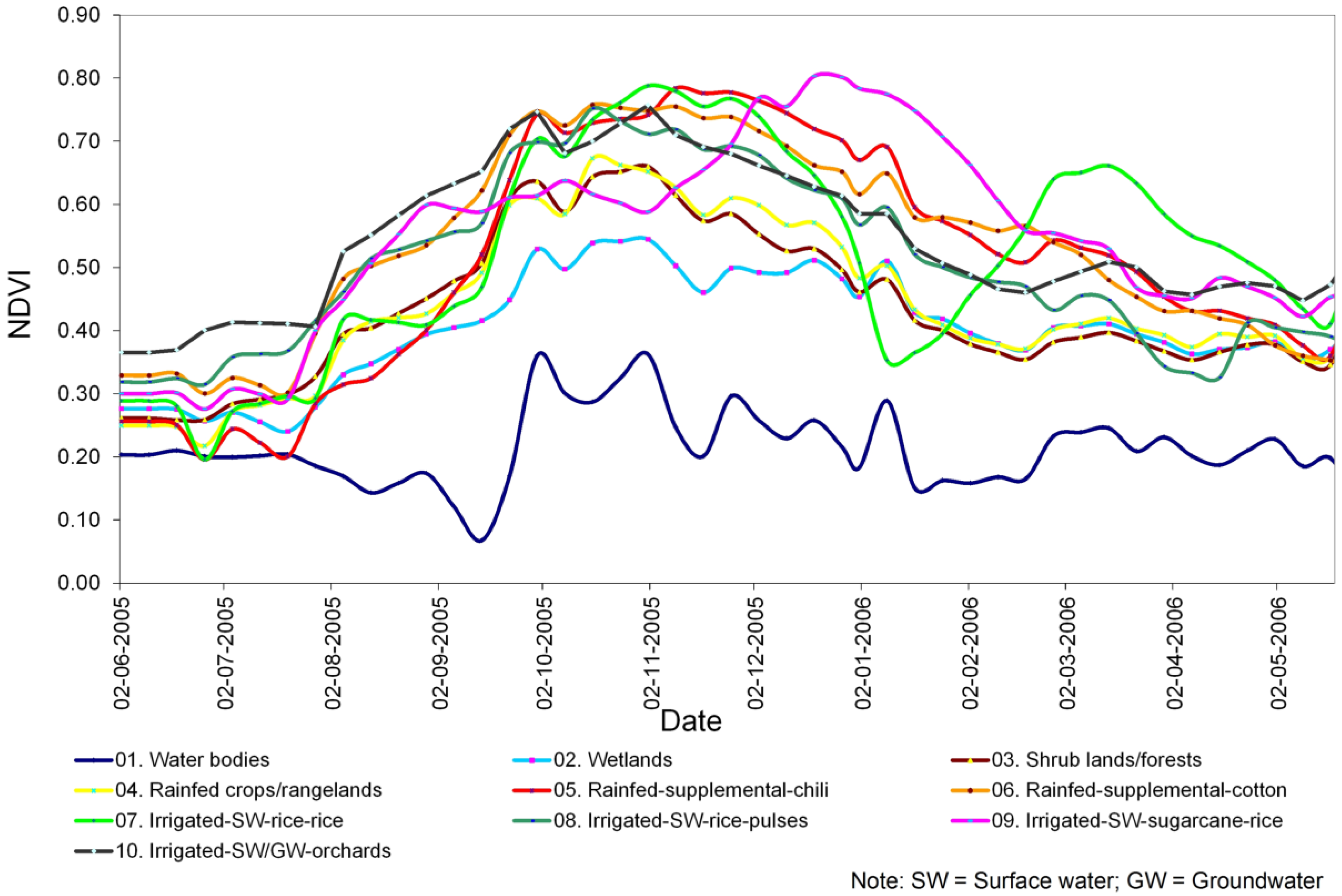
4.2. Temporal Signature of Various Land Use Classes
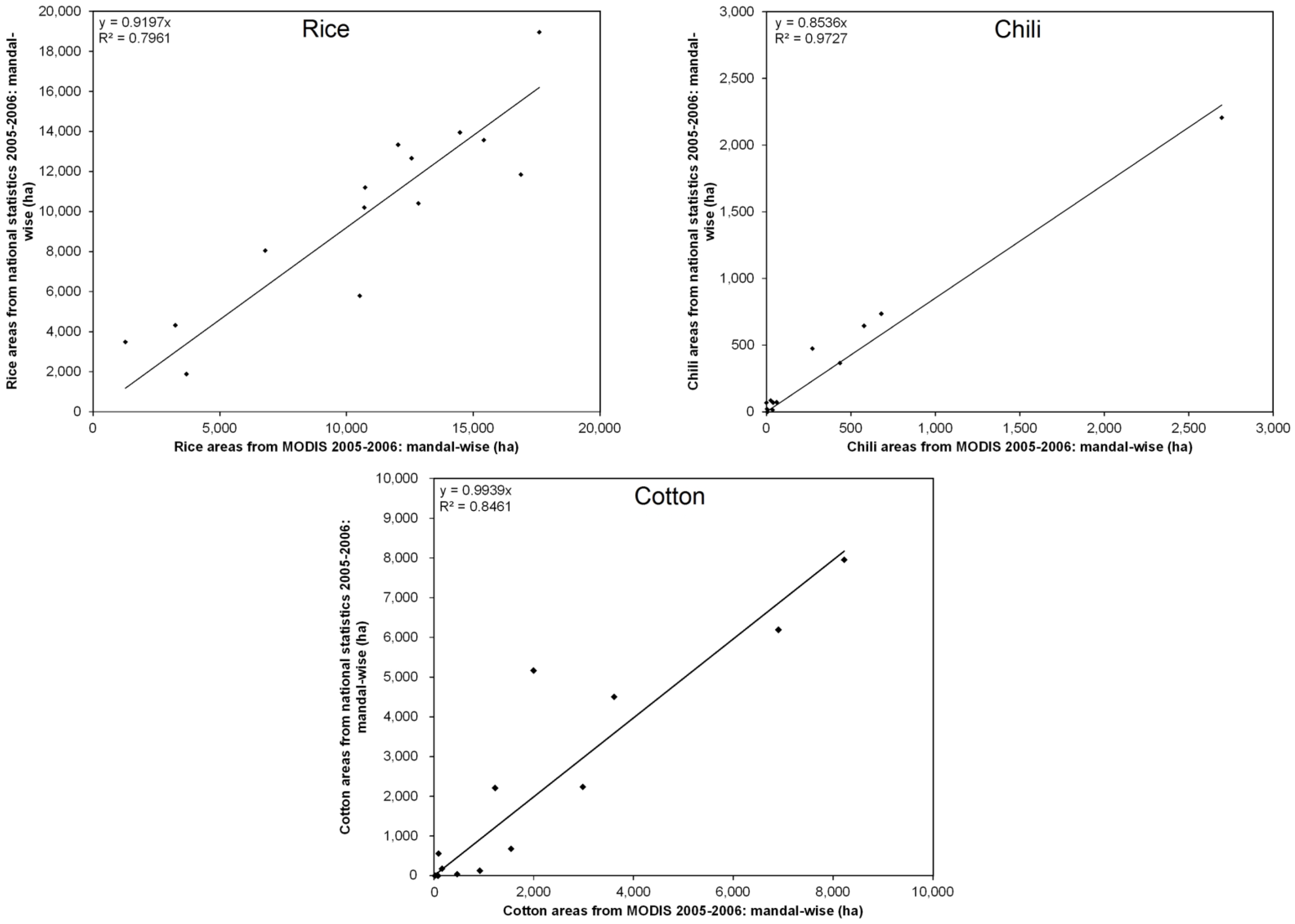
4.3. Comparisons with National Statistics and Other Studies
| Mandals | Area (ha) | % Difference | |||||||
|---|---|---|---|---|---|---|---|---|---|
| MODIS Rice | NAS Rice | MODIS Cotton | NAS Cotton | MODIS Chili | NAS Chili | Rice | Cotton | Chili | |
| Peddavoora | 3,688 | 3,879 | 3,613 | 4,500 | 436 | 365 | 5 | 20 | −19 |
| Nidamnoor | 15,422 | 13,569 | 1,226 | 1,208 | 40 | 67 | −14 | −1 | 41 |
| Neredcherla | 17,611 | 18,957 | 1,549 | 1,675 | 272 | 474 | 7 | 8 | 43 |
| Nadigudem | 3,246 | 4,315 | 161 | 175 | 3 | 20 | 25 | 8 | 83 |
| Munagala | 1,276 | 3,480 | 94 | 555 | 0 | 0 | 63 | 83 | 0 |
| Miryalaguda | 16,882 | 11,843 | 466 | 379 | 37 | 34 | −43 | −23 | −7 |
| Mellachervu | 12,569 | 12,660 | 8,224 | 7,954 | 2,695 | 2,205 | 1 | −3 | −22 |
| Mattampally | 10,527 | 9,785 | 2,984 | 2,234 | 578 | 644 | −8 | −34 | 10 |
| Kodad | 14,476 | 13,947 | 920 | 926 | 25 | 84 | −4 | 1 | 70 |
| Huzurnagar | 10,737 | 11,200 | 0 | 0 | 6 | 0 | 4 | 0 | 0 |
| Garidepally | 12,843 | 10,400 | 0 | 8 | 5 | 0 | −23 | 0 | 0 |
| Damercherla | 12,037 | 13,337 | 6,904 | 6,192 | 681 | 735 | 10 | −12 | 7 |
| Chilkur | 6,794 | 8,050 | 23 | 0 | 6 | 0 | 16 | 0 | 0 |
| Anumula | 10,704 | 10,201 | 1,998 | 5,166 | 61 | 72 | −5 | 61 | 15 |
| Total | 148,811 | 145,623 | 28,162 | 30,972 | 4,843 | 4,700 | 2 | 8 | 16 |
4.4. Comparison with Other Studies
| Land Use Class# | Area in ha | ||
|---|---|---|---|
| MODIS 500 m [41] | MODIS 250 m [42] | IRS-P6 + MODIS 250 m (Present Study) | |
| Left bank | |||
| Irrigated agriculture | 422,196 | 561,900 | 556,657 |
| Rainfed: supplemental | 220,276 | 100,500 | 158,880 |
| Rainfed agriculture | 183,563 | 56,100 | 63,744 |
| Right bank | |||
| Irrigated agriculture | - | 282,200 | 287,310 |
| Rainfed—supplemental | - | 327,400 | 387,184 |
| Rainfed agriculture | - | 137,500 | 94,940 |
4.5. Accuracy Assessment through Error Matrix
4.6. Utility of These Maps in Decision-Making

| 01 | 02 | 03 | 04 | 05 | 06 | 07 | 08 | 09 | 10 | Reference Totals | Number Correct | Producers Accuracy | Users Accuracy | |
| 01 | 3 | 0 | 0 | 0 | 0 | 0 | 0 | 0 | 0 | 0 | 3 | 3 | 100% | 100% |
| 02 | 0 | 5 | 0 | 0 | 0 | 0 | 0 | 0 | 0 | 0 | 5 | 5 | 100% | 100% |
| 03 | 0 | 0 | 2 | 0 | 0 | 0 | 1 | 0 | 0 | 0 | 2 | 2 | 100% | 67% |
| 04 | 0 | 0 | 0 | 6 | 1 | 0 | 2 | 0 | 0 | 0 | 7 | 6 | 86% | 67% |
| 05 | 0 | 0 | 0 | 1 | 4 | 1 | 1 | 0 | 0 | 0 | 6 | 4 | 67% | 57% |
| 06 | 0 | 0 | 0 | 0 | 1 | 11 | 0 | 1 | 0 | 0 | 13 | 11 | 85% | 85% |
| 07 | 0 | 0 | 0 | 0 | 0 | 1 | 17 | 0 | 1 | 1 | 25 | 17 | 68% | 85% |
| 08 | 0 | 0 | 0 | 0 | 0 | 0 | 2 | 7 | 0 | 1 | 8 | 7 | 88% | 70% |
| 09 | 0 | 0 | 0 | 0 | 0 | 0 | 1 | 0 | 3 | 0 | 4 | 3 | 75% | 75% |
| 10 | 0 | 0 | 0 | 0 | 0 | 0 | 1 | 0 | 0 | 6 | 8 | 6 | 75% | 86% |
| Column Total | 3 | 5 | 2 | 7 | 6 | 13 | 25 | 8 | 4 | 8 | 81 | 64 |
5. Conclusions
Acknowledgments
Author Contributions
Conflicts of Interest
References
- Oetter, D.R.; Cohen, W.B.; Berterretche, M.; Maiersperger, T.K.; Kennedy, R.E. Land cover mapping in an agricultural setting using multiseasonal thematic mapper data. Remote Sens. Environ. 2001, 76, 139–155. [Google Scholar] [CrossRef]
- Gumma, M.K.; Nelson, A.; Thenkabail, P.S.; Singh, A.N. Mapping rice areas of south asia using modis multitemporal data. J. Appl. Remote Sens. 2011, 5. [Google Scholar] [CrossRef]
- Thiruvengadachari, S.; Murthy, C.S.; Raju, P.V. Remote Sensing of Bhankra Canal Command Area, Harayana, India; NRSA: Hyderabad, India, 1997. [Google Scholar]
- Thiruvengadachari, S.; Sakthivadivel, R. Satellite Remote Sensing for Assessment of Irrigation System Performance: A Case Study in India; Research Report 9; International Irrigation Management Institute: Colombo, Sri Lanka, 1997. [Google Scholar]
- Bastiaanssen, W.G.M.; Bos, M.G. Irrigation performance indicators based on remotely sensed data: A review of literature. Irrig. Drain. Syst. 1999, 13, 291–311. [Google Scholar] [CrossRef]
- Ambast, S.K.; Keshari, A.K.; Gosain, A.K. Satellite remote sensing to support management of irrigation systems: Concepts and approaches. Irrig. Drain. 2002, 51, 25–39. [Google Scholar] [CrossRef]
- Bastiaanssen, W.G.M.; Molden, D.J.; Thiruvengadachari, S.; Smit, A.A.M.F.R.; Mutuwatte, L.; Jayasinghe, G. Remote Sensing and Hydrologic Models for Performance Assessment in Sirsa Irrigation Circle, India; International Water Management Institute: Patancheru, India, 1999. [Google Scholar]
- Ozdogan, M.; Woodcock, C.E.; Salvucci, G.D. Monitoring changes in summer irrigated crop area in southeastern turkey using remote sensing. In Proceedings of the 2003 IEEE International Geoscience and Remote Sensing Symposium, IGARSS, Melborne, Australia, 21–25 July 2003; pp. 1570–1572.
- Sakthivadivel, R.; Thiruvengadachari, S.; Amerasinghe, U.; Bastiaanssen, W.G.M.; Molden, D. Performance Evaluation of the Bhakra Irrigation System, India, Using Remote Sensing and Gis Techniques; International Water Management Institute: Colombo, Sri Lanka, 1999. [Google Scholar]
- Velpuri, N.M.; Thenkabail, P.S.; Gumma, M.K.; Biradar, C.B.; Noojipady, P.; Dheeravath, V.; Yuanjie, L. Influence of resolution in irrigated area mapping and area estimations. Photogramm. Eng. Remote Sens. 2009, 75, 1383–1395. [Google Scholar] [CrossRef]
- Gumma, M.K.; Thenkabail, P.S.; Hideto, F.; Nelson, A.; Dheeravath, V.; Busia, D.; Rala, A. Mapping irrigated areas of ghana using fusion of 30 m and 250 m resolution remote-sensing data. Remote Sens. 2011, 3, 816–835. [Google Scholar] [CrossRef]
- Biggs, T.W.; Thenkabail, P.S.; Gumma, M.K.; Scott, C.A.; Parthasaradhi, G.R.; Turral, H.N. Irrigated area mapping in heterogeneous landscapes with modis time series, ground truth and census data, Krishna Basin, India. Int. J. Remote Sens. 2006, 27, 4245–4266. [Google Scholar] [CrossRef]
- Draeger, W.C. Monitoring irrigated land acreage using landsat imagery: An application example. In Proceedings of the ERIM 11th International Symposium on Remote Sensing of Environment, Las Vegas, NV, USA, 1977; SEE N78-14464 05-43. pp. 515–524.
- Rundquist, D.C.; Richardo, H.; Carlson, M.P.; Cook, A. The nebraska center-pivot inventory—An example of operational satellite remote sensing on a long term basis. Photogramm. Eng. Remote Sens. 1989, 55, 587–590. [Google Scholar]
- Thiruvengadachari, S. Satellite sensing of irrigation pattern in semiarid areas: An indian study. Photogramm. Eng. Remote Sens. 1981, 47, 1493–1499. [Google Scholar]
- Abderrahman, W.A.; Bader, T.A. Remote sensing application to the management of agricultural drainage water in severely arid region: A case study. Remote Sens. Environ. 1992, 42, 239–246. [Google Scholar] [CrossRef]
- Murthy, C.S.; Raju, P.V.; Jonna, S.; Hakeem, K.A.; Thiruvengadachari, S. Satellite derived crop calendar for canal operation schedule in bhadra project command area, India. Int. J. Remote Sens. 1998, 19, 2865–2876. [Google Scholar] [CrossRef]
- Thenkabail, P.S.; Biradar, C.M.; Turral, H.; Noojipady, P.; Li, Y.; Vithanage, J.; Dheeravath, V.; Velpuri, M.; Schull, M.; Cai, X.; et al. An Irrigated Area Map of the World (1999) Derived from Remote Sensing; Research Report 105; International Water Management Institute: Colombo, Sri Lanka, 2006. [Google Scholar]
- Alexandridis, T.; Asi, S.; Ali, S. Water Performance Indicators Using Satellite Imagery for the Fordwah Eastern Sadiqia (South) Irrigation and Drainage Project; International Water Management Institute: Colombo, Sri Lanka, 1999; p. 16. [Google Scholar]
- Boken, V.K.; Hoogenboom, G.; Kogan, F.N.; Hook, J.E.; Thomas, D.L.; Harrison, K.A. Potential of using noaa-avhrr data for estimating irrigated area to help solve an inter-state water dispute. Int. J. Remote Sens. 2004, 25, 2277–2286. [Google Scholar] [CrossRef]
- Thenkabail, P.S.; Schull, M.; Turral, H. Ganges and indus river basin land use/land cover (LULC) and irrigated area mapping using continuous streams of modis data. Remote Sens. Environ. 2005, 95, 317–341. [Google Scholar] [CrossRef]
- Kamthonkiat, D.; Honda, K.; Turral, H.; Tripathi, N.K.; Wuwongse, V. Discrimination of irrigated and rainfed rice in a tropical agricultural system using spot vegetation ndvi and rainfall data. Int. J. Remote Sens. 2005, 26, 2527–2547. [Google Scholar] [CrossRef]
- Gumma, M.K.; Mohanty, S.; Nelson, A.; Arnel, R.; Mohammed, I.A.; Das, S.R. Remote sensing based change analysis of rice environments in Odisha, India. J. Environ. Manag. 2014, in press. [Google Scholar]
- Knight, J.F.; Lunetta, R.L.; Ediriwickrema, J.; Khorram, S. Regional scale land-cover characterization using modis-ndvi 250 m multi-temporal imagery: A phenology based approach. GIScience Remote Sens. 2006, 43, 1–23. [Google Scholar] [CrossRef]
- Krishna Water Disputes Tribunal. Further Report of the Krishna Water Disputes Tribunal; Government of India: New Delhi, India, 1976; p. 109.
- Van Rooijen, D.; Turral, H.; Biggs, T.W. Sponge city: Water balance of mega-city water use and wastewater use in Hyderabad, India. Irrig. Drain. 2005, 54, S81–S91. [Google Scholar] [CrossRef]
- Thenkabail, P.S.; Enclona, E.A.; Ashton, M.S.; Legg, C.; de Dieu, M.J. Hyperion, IKONOS, ALI, and ETM+ sensors in the study of African rainfores. Remote Sens. Environ. 2004, 90, 23–43. [Google Scholar] [CrossRef]
- Markham, B.L.; Barker, J.L. Landsat MSS and TM Post- Calibration Dynamic Ranges, Exoatmospheric Reflectances and At-Satellite Temperatures; Landsat Technical Notes, 1; Earth Observation Satellite Company: Lanham, Maryland, August 1986. [Google Scholar]
- Neckel, H.; Labs, D. The solar radiation between 3300 and 12500 Å. Sol. Phys. 1984, 90, 205–258. [Google Scholar]
- International water management insttitute data store house pathway (IWMIDSP). Available online: http://www.iwmidsp.org (accessed on 12 December 2010).
- NASA, MODIS data, Moderate Resolution Imaging Spectrometer (MODIS). Available online: http://modis-land.gsfc.nasa.gov (accessed on 25 August 2013).
- Gumma, M.K.; Thenkabail, P.S.; Maunahan, A.; Islam, S.; Nelson, A. Mapping seasonal rice cropland extent and area in the high cropping intensity environment of bangladesh using modis 500 m data for the year 2010. ISPRS J. Photogramm. Remote Sens. 2014, 91, 98–113. [Google Scholar] [CrossRef]
- NASA, Geo cover 2000. Available online: https://zulu.ssc.nasa.gov/mrsid/ (accessed on 25 August 2013).
- Gumma, M.K.; Gauchan, D.; Nelson, A.; Pandey, S.; Rala, A. Temporal changes in rice-growing area and their impact on livelihood over a decade: A case study of nepal. Agric. Ecosyst. Environ. 2011, 142, 382–392. [Google Scholar] [CrossRef]
- Gumma, M.K.; Thenkabail, P.S.; Muralikrishna, I.V.; Velpuri, M.N.; Gangadhararao, P.T.; Dheeravath, V.; Biradar, C.M.; Acharya Nalan, S.; Gaur, A. Changes in agricultural cropland areas between a water-surplus year and a water-deficit year impacting food security, determined using modis 250 m time-series data and spectral matching techniques, in the Krishna River Basin (India). Int. J. Remote Sens. 2011, 32, 3495–3520. [Google Scholar] [CrossRef]
- Thenkabail, P.S.; GangadharaRao, P.; Biggs, T.; Gumma, M.K.; Turral, H. Spectral matching techniques to determine historical land use/land cover (lulc) and irrigated areas using time-series avhrr pathfinder datasets in the Krishna River Basin, India. Photogramm. Eng. Remote Sens. 2007, 73, 1029–1040. [Google Scholar]
- Gumma, M.K.; Thenkabail, P.S.; Nelson, A. Mapping irrigated areas using modis 250 meter time-series data: A study on Krishna River Basin (India). Water 2011, 3, 113–131. [Google Scholar] [CrossRef]
- Jensen, J.R. Introductory Digital Image Processing: A Remote Sensing Perspective, 3rd ed.; Prentice Hall: Upper Saddle River, NJ, USA, 2004; p. 544. [Google Scholar]
- Congalton, R.G. A review of assessing the accuracy of classifications of remotely sensed data. Remote Sens. Environ. 1991, 37, 35–46. [Google Scholar] [CrossRef]
- Congalton, R.G.; Green, K. Assessing the Accuracy of Remotely Sensed Data: Principles and Practices; CRC Press: New York, NY, USA, 1999. [Google Scholar]
- Gaur, A.; Biggs, T.W.; Gumma Murali, K.; Pardhasaradhi, G.; Turral, H. Water scarcity effects on equitable water distribution and land use in major irrigation project—A case study in India. J. Irrig. Drain. Eng. 2008, 134, 26–35. [Google Scholar] [CrossRef]
- Venot, J.-P.; Jella, K.; Bharati, L.; George, B.; Biggs, T.; Rao, P.G.; Gumma, M.K.; Acharya, S. Farmers’ adaptation and regional land-use changes in irrigation systems under fluctuating water supply, south India. J. Irrig. Drain. Eng. 2010, 136, 595–609. [Google Scholar] [CrossRef]
© 2014 by the authors; licensee MDPI, Basel, Switzerland. This article is an open access article distributed under the terms and conditions of the Creative Commons Attribution license (http://creativecommons.org/licenses/by/3.0/).
Share and Cite
Gumma, M.K.; Pyla, K.R.; Thenkabail, P.S.; Reddi, V.M.; Naresh, G.; Mohammed, I.A.; Rafi, I.M.D. Crop Dominance Mapping with IRS-P6 and MODIS 250-m Time Series Data. Agriculture 2014, 4, 113-131. https://doi.org/10.3390/agriculture4020113
Gumma MK, Pyla KR, Thenkabail PS, Reddi VM, Naresh G, Mohammed IA, Rafi IMD. Crop Dominance Mapping with IRS-P6 and MODIS 250-m Time Series Data. Agriculture. 2014; 4(2):113-131. https://doi.org/10.3390/agriculture4020113
Chicago/Turabian StyleGumma, Murali Krishna, Kesava Rao Pyla, Prasad S. Thenkabail, Venkataramana Murthy Reddi, Gundapaka Naresh, Irshad A. Mohammed, and Ismail M. D. Rafi. 2014. "Crop Dominance Mapping with IRS-P6 and MODIS 250-m Time Series Data" Agriculture 4, no. 2: 113-131. https://doi.org/10.3390/agriculture4020113