Economic Analysis of Organic Rankine Cycle Using R123 and R245fa as Working Fluids and a Demonstration Project Report


1
Key Laboratory of Enhanced Heat Transfer and Energy Conservation, Ministry of Education, College of Environmental and Energy Engineering, Beijing University of Technology, Beijing 100124, China
2
Key Laboratory of Heat Transfer and Energy Conversion, Beijing Municipality, College of Environmental and Energy Engineering, Beijing University of Technology, Beijing 100124, China
*
Author to whom correspondence should be addressed.
Appl. Sci. 2019, 9(2), 288; https://doi.org/10.3390/app9020288
Submission received: 27 November 2018
/
Revised: 5 January 2019
/
Accepted: 10 January 2019
/
Published: 15 January 2019
(This article belongs to the Special Issue Organic Rankine Cycle Systems for Waste-Heat Recovery)
Abstract
:Featured Application
The results introduced in this work can offer a good suggestion for the construction of actual organic Rankine cycle system from an economic point of view.
Abstract
The organic Rankine cycle (ORC) is a popular technology used in waste heat recovery and low-grade heat utilization, which are two important measures to solve the problems brought by the energy crisis. The economic performance of ORC system is an important factor affecting its application and development. Therefore, the economic analysis of ORC is of great significance. In this study, R123 and R245fa, two frequently-used working fluids during the transition period, were selected for calculating and analyzing the economic performance of an ORC used for recovery of waste heat with a low flow rate and medium-low temperature. Five traditional economic indicators, namely total cost, net earnings, payback period, return on investment, levelized energy cost, and present value of total profit in system service life, which is a relatively new indicator, were used to establish the economic analysis model of ORC. The variation effects of evaporation temperature, condensation temperature of working fluid, flue gas inlet temperature, and mass flow rate of flue gas on the above six economic indicators were analyzed. The results show that the optimal evaporation temperature of R123 is 125 °C, the optimal condensation temperature is 33 °C, and the optimal heat source temperature is 217 °C. For R245fa, the optimal evaporation temperature is 122 °C, the optimal condensation temperature is 27 °C, and the optimal heat source temperature is 177 °C. The economic performance of an ORC demonstration project was reported and used for comparison with the estimation and analysis. It was found that the single screw expander has an excellent economy performance, which greatly reduces the proportion of expander cost in the ORC system.
1. Introduction
Energy consumption has greatly contributed to the promotion of human development and progress. However, its waste emission brings more and more serious environmental pollution and ecological destruction simultaneously. Waste heat recovery and low-grade heat utilization are important measures to solve the problems brought by energy consumption. The organic Rankine cycle (ORC), which applies the principle of the steam Rankine cycle but uses organic working fluids with low boiling points, is a very promising technique used for waste heat recovery. The group of Lemort and Quoilin [1] focused on both the thermodynamic and economic optimization of a small scale ORC in waste heat recovery application. The working fluids they considered include R245fa, R123, n-butane, n-pentane, R1234yf and Solkatherm. They also carried out experimental study using scroll expander and using R123 [2] and R245fa [3]. The group of Karellas conducted much research on ORC configuration optimization [4,5,6] and experimental performance [7]. The group of Brüggemann, Heberle, and Preißinger used isobutane/isopentane and R227ea/R245fa as working fluids in ORC for low-enthalpy geothermal resources [8] and conducted a thermoeconomic analysis [9]. They also carried out an experimental characterization and comparison of axial and cantilever micro-turbines for small-scale ORC [10]. Many papers focus on internal combustion engine (ICE) waste heat recovery using ORC technique [11,12,13,14,15,16,17]. Cycle configurations [11,12,16,17], fluids [14,15] and parameters optimization [13,14,15] are usually discussed and analyzed in these papers. However, there are few reports on test bench or experimental system used for ICE waste heat recovery based on ORC technique.
Among the four devices making up an ORC, the expander is the critical component because it determines the efficiency and cost of an ORC. Expanders, in general, can be categorized into two types: the velocity type and the volume type. The popular axial turbine expanders belong to the former type while the latter type includes screw expanders, scroll expanders and reciprocal piston expanders [18]. Yamada et al. [19] developed a compact ORC system using a compact rotary-vane-type expander for low-temperature waste heat recovery. Approximately 30 W of expander power output with 48% expander efficiency was achieved. Kolasi’nski et al. [20] conducted experimental and numerical analyses on the rotary vane expander in a micro ORC system. They indicated that a properly designed multi-vane expander is a cheap and mechanically simple alternative to other expansion devices proposed for domestic ORC systems [21]. The group of Lemort and Quoilin [2,3] modified a scroll compressor to an expander and conducted experimental studies. Measured performance on the prototype is very promising in a wide range of operating conditions. The maximum shaft power is 2.1 kW and maximum achieved isentropic efficiency is 75.7% [3]. Bao and Zhao [22] carried out a detailed review on the expander used in ORC. They summarized the prototype research on various types of expansion machines. They also made a comparison of various types of expanders suitable for ORC system. According to the power capacity, radial-inflow turbine is maximum, which is suitable for the large capacity system. For volume type expander, screw and reciprocating piston expanders can also output relatively high power, which can be applied to small- and medium-sized systems. The capacity of scroll and rotary vane expander is minimum, generally applied in small- or micro-ORC systems. In general, the selection of expansion machines should consider many factors, such as the power capacity, isentropic efficiency, cost, complexity, etc., and different expansion machines have their own applicable scope so that reasonable selection is based on system operation and working conditions.
In ORC, organic working fluid plays a decisive role. The working fluid selection can greatly affect economic feasibility of an ORC while the economic performance of ORC system is an important factor affecting its application and development. Moreover, the impact on the environment is also greatly affected by working fluid selection. From a historical perspective, chlorofluorocarbons (CFCs) and hydrochlorofluorocarbons (HCFCs) dominated organic working fluids from 1931 to the early 1990s. Since the ratification of the Montreal Protocol in 1987 and the Kyoto Protocol in 1997, more and more attention has been paid to the development of environmentally friendly organic working fluids. Therefore, based on environmental concerns, CFC working fluids have been phased out and HCFC working fluids will be phased out by 2040 for developing countries. Hydrofluoroolefins (HFO) working fluids are drawing more and more attention. During the transition period, R123 (HCFC working fluid) [23,24,25,26,27,28,29,30] and R245fa (HFC working fluid) [24,25,26,27,31,32,33,34] are two frequently-used working fluids in ORC. Therefore, the economic analysis of ORC utilizing R123 and R245fa is of great significance. Especially for developing countries, many ORC systems using R123 or R245fa as working fluids are in use or in development.
One of the first articles focusing on exergoeconomic analyses was carried out by Tsatsaronis in the 1980s [35]. Afterwards, much research on economic analysis of thermodynamic cycle system has been conducted from different aspects. Different methods and equations have been developed and proposed accordingly. Kim et al. [36] developed an exergy-costing method by assigning a single unit cost to a specific exergy, regardless of the type of exergy stream and state of the stream. Applying the cost-balance equation to each component of a 1000 kW gas turbine cogeneration system, they obtained exergy costs, production cost of electricity, and the lost costs of each component of the system. Based on the Specific Exergy Costing (SPECO) approach, Lazzaretto and Tsatsaronis [37] proposed a systematic and general methodology for defining and calculating exergetic efficiencies and exergy related costs in thermal systems. They introduced some guidelines that can generalize and simplify the definitions of exergetic efficiencies and the costing procedures. Those guidelines significantly reduce the arbitrariness in applications of exergy costing. Using levelized energy cost (LEC) as an economic indictor, Zhang et al. [38] conducted a performance comparison and parametric optimization of subcritical ORC and transcritical power cycle system for low-temperature geothermal power generation. They found that, although the thermal efficiency and exergy efficiency of R125 in transcritical cycle is 46.4% and 20% lower than that of R123 in subcritical ORC, it provides 20.7% larger recovery efficiency. The LEC value is relatively low. Moreover, 22032L petroleum is saved and 74,019 kg CO2 is reduced per year when the LEC value is used as the objective function. Abusoglu and Kanoglu [39] discussed the concepts of exergetic cost and cost accounting methods, and conducted a brief historical overview on the exergoeconomic analysis and optimization of combined heat and power production (CHPP). Compared with conventional energy analysis, these methods can solve problems related to complex energy systems. Vélez et al. [40] presented an overview of the technical and economic aspects, as well as the market evolution of the Organic Rankine Cycle (ORC). In their research, because of the lack of any real installations to show the cost, a simple economic analysis has been carried out to find the maximum investment that a project can assume when the return on investment is required in a year. Fiaschi et al. [41] used investment and operation and maintenance (O&M) costs as the indicators to analyze and compare exergoeconomic performance of ORC and Kalina cycles, which are used to exploit low and medium-high temperature heat from two different geothermal sites. Yari et al. [42] used capital recovery factor (CRF) as the indicator to conduct an exergoeconomic comparison of TLC (trilateral Rankine cycle), ORC and Kalina cycle using a low-grade heat source. They found that, although the TLC can achieve a higher net output power compared with ORC and Kalina (KCS11 (Kalina cycle system 11)) systems, its product cost is greatly affected by the expander isentropic efficiency. They also observed that, for both ORC and Kalina systems, the optimum operating condition for maximum net output power differs from that for minimum product cost. Meinel et al. [43] compared economic performance of ORC processes at different scales using purchased equipment costs (PEC), maintenance and operating costs (MO), and capital investment cost (CIC) as the indicators. Esen et al. [44] used the annual cost method to make a technoeconomic comparison of ground-coupled and air-coupled heat pump system for space cooling. Purchase cost and payback period [45] were used by Varga and Csaba as the indicators to conduct a techno-economic evaluation of waste heat recovery by organic Rankine cycle using pure light hydrocarbons and their mixtures as working fluid in a crude oil refinery. Luo et al. [46] used total capital investment as the indicator to make a thermo-economic analysis and optimization of a zoetropic fluid organic Rankine cycle with liquid–vapor separation during condensation.
Based on the reviewed papers, it can be seen that different indicators are used to evaluate the economic performance of different thermodynamic systems. However, many indicators are proposed for a particular process or system or, in most work, only one or two indicators are used. Therefore, in this work, five traditional and classical indicators, namely total cost, net earnings, payback period, return on investment, and levelized energy cost, were selected for thermo-economic analysis of ORC using R123 and R245fa as working fluid. Considering that the above five indicators mainly focus on the present economic performance evaluation, a new indicator, which is called present value of total profit in system service life, is proposed. This new indicator can be used to evaluate the economic performance of engineering technology solution throughout its service life. Using these six indicators, the thermo-economic evaluation model of ORC with R123 and R245fa was established and the variation effect of influencing factor on system economic performance was calculated and analyzed. Herein, the economic performance of an ORC demonstration project is reported.
2. Methods
2.1. Thermodynamic Parameter Setting and Calculation
ORC is usually used in low-medium temperature waste heat recovery. Table 1 gives the temperatures of waste gases from process equipment in the low-medium temperature range. Figure 1 depicts the typical process of an ORC, in which dry and isentropic working fluids are always used as working fluids. After isentropic expansion process to produce work, the dry working fluid with a positive slope of the saturation vapor curve is at a superheated state and the isentropic working fluid with a nearly infinitely large slope is at a saturated state. This avoids blade damage of the turbine caused by wet vapor. To simplify the calculation, the following assumptions were made. (1) All processes are quasi-stationary processes. (2) The pressure loss of pipes and heat exchangers are ignored. The efficiencies of the expander and pump are 0.8. (3) There is no superheating in ORC [47]. Table 2 gives some parameter settings for thermodynamic calculation.
In our analysis, tube-in-tube heat exchanger was adopted due to the following advantages.
- (1)
- The structure is simple and the heat transfer area can be increased or decreased freely. Because it is composed of standard components, no additional processing is required for installation.
- (2)
- It has a high heat transfer efficiency. It is a counter-flow heat exchanger. Appropriate cross-section size can be set for improving the fluid speed and increasing the heat transfer coefficient of both sides of the fluid.
- (3)
- It has a wide working range. The shape can be changed arbitrarily according to the installation position to facilitate installation.
In evaporator, organic working fluid flows in inner tube and flue gas flows in outer tube. Water is used in condenser and its temperature is 15 °C, which is the same as the ambient temperature. When the mass flow rate and inlet temperature of heat source are given, the mass flow rate of organic working fluid and outlet temperature of heat source can be determined by pinch point temperature difference method. Similarly, the mass flow rate and outlet temperature of cooling water can be determined by giving inlet temperature of cooling water.
The parameters can be calculated by the following equations.
The mass flow of organic working fluid,
The outlet temperature of heat source,
The mass flow of cooling water,
The outlet temperature of cooling water,
In evaporator and condenser, the heat transfer includes single-phase and vapor–liquid phase process. During single-phase heat transfer process, heat convection coefficients of organic working fluid in tube and fluid outside the tube can be calculated according to Dittus–Boelter equation.
where α is heat convection coefficient. When fluid is heated, n = 0.4. When cooled, n = 0.3. Mean temperature of inlet and outlet was adopted as qualitative temperature. (D − d), the difference between inner tube diameter and outer tube diameter, was adopted as characteristic dimension.
In evaporator, heat convection coefficients of organic working fluid during vapor–liquid heat transfer process can be calculated by the following equation [52].
where Bo is boiling characteristic number, x is vapor quality, x = 0.5. Mean temperature was used as qualitative temperature. Characteristic dimension is d.
In condenser, heat convection coefficients of organic working fluid during vapor–liquid heat transfer process can be calculated by the following equation [53].
where mean temperature was used as qualitative temperature. Characteristic dimension is d. x = 0.5.
In evaporator and condenser, the heat transfer during single-phase and vapor–liquid phase process is calculated by the following equation.
Logarithmic mean temperature difference is calculated by
In evaporator and condenser, the heat transfer coefficient is calculated by
where λF is heat conductivity of steel.
In evaporator and condenser, convective heat transfer area is calculated by
The area of evaporator is calculated by
The area of condenser is calculated by
The total area of heat exchanger is
2.2. Economic Indicators and Calculations
The investment in ORC includes two parts: equipment investment and working fluid investment. Equipment investment includes investment in evaporator, condenser, expander, and pump. The calculations of investment in evaporator and condenser are based on their heat exchanger areas. The calculations of investment in pump and expander are based on their capacity. The working fluid investment is calculated by the quality of working fluid that can be accommodated by the evaporator and condenser chamber and the system piping.
The purchased cost of heat exchanger can be estimated by the following equation [54].
The purchased cost of pump and expander can be estimated by the following equation [54].
In Equations (17) and (18), Cp is basic purchased cost. Bare module cost of equipment after material and pressure corrections is estimated by
where FM is material factor and Fp is pressure factor.
Pressure factor can be calculated by
In the above equations, K1, K2, K3, B1, B2, C1, C2, and C3 are all correction factors. Their values for purchased cost calculation of heat exchanger are listed in Table 3. Those values for pump and expander are listed in Table 4. The uncertainty was quantified via a scenario analysis [54].
To consider the effects of inflation on equipment costs, the Chemical Engineering Plant Cost Index (CEPCI) was adopted for all inflation adjustments. Therefore, bare module cost of equipment in 2016 can be estimated by
The bare module cost of working fluid is estimated by
where pw is the unit price of working fluid. Mw is the mass of working fluid and it is obtained by multiplying the volume of working fluid determined by the heat exchanger chamber and the system piping by the density of working fluid. In this work, the unit price of R123 was 17.967 $/kg, R245fa was 14.81 $/kg.
2.2.1. Total Cost of ORC System
Total cost of ORC system is estimated by
where CBM,e is investment in evaporator, CBM,c is investment in condenser, CBM,p is investment in pump, CBM,ex is investment in expander, and CBM,w is investment in working fluid.
2.2.2. Net Earnings (NE) of ORC System
Net Earnings (NE) of ORC System is the annual net output power multiplied by the unit grid price. The annual net output power of ORC system refers to the output power of expander minus the work consumed by pump.
where pe is the unit grid price whose value is 0.1 $/kW·h. top is annual operation time of system, taken as 8000 h here.
2.2.3. Payback Period (PP) of ORC System
The payback period (PP) is the time required to make the accumulated economic benefit equal to the initial investment cost. The dynamic investment payback period is obtained by converting the net cash flow of each year of the investment into the present value based on the benchmark rate of return.
Payback Period is estimated by
where cost of maintenance (COM) accounts for 1.5% of total cost of ORC system, COM = 1.5%Ctot. Annual interest rate was set as i = 5%.
2.2.4. Return on Investment (ROI) of ORC System
The return on investment (ROI) is the ratio of the Net Earnings (NE) to the Total Cost of ORC System. It is estimated by
2.2.5. Levelized Energy Cost (LEC) of ORC System
Levelized Energy Cost (LEC) presents the average power generation cost per kWh. It is calculated by considering compound interest of total cost of system and the operation and maintenance costs.
where Wex is the output power of expander, Wp is the work consumed by pump, i is bank interest rate, and Ts is system service life, taken as 20 years here.
2.2.6. Present Value of Total Profit in System Service Life
The above five indicators mainly focus on the present economic performance evaluation of ORC system. However, for an engineering technology solution, the evaluation of present economic performance is not enough. The economic performance of a solution throughout its service life should be evaluated.
We usually use monetary units to evaluate engineering solutions, so in the economic analysis we mainly focused on the cash flow of the income and expenditure of the equipment (solution) throughout its service life. Can we add up the cash flows that occur throughout the service life directly? No, this is because the payment effect of money is not only related to the amount of money, but also to the time of occurrence. The value of $5 received this year is different from that of $5 that will be received next year. Even if inflation is not considered, its value is different because the initial earned money can be turned into funds for investment and generates new value. This is called the time value of money. The longer the time lasts, the greater value is added. Because the value of money varies with time, cash flows that occur at different times cannot be directly added and compared. In this way, the economic analysis and the comparison between different technological and economic solutions become more complicated. It is necessary to make a currency equivalent calculation with time factor, that is, calculate the cash flow at various times according to the bank interest formula. For a technical solution with a long payback period and complicated system, a dynamic analysis method considering the time value of funds can be adopted, and a fixed discount rate can be used to convert the future value in solution service life into present value to evaluate the economy performance of the technical solution.
If an ORC system is built for waste heat recovery, the total net profit earned from the commissioning to the service life of the system can be considered. Regardless of the initial investment, the annual net profit is net income minus operation and maintenance costs. In this way, the profits are the same every year. However, if interest rate is considered, the value of the same amount of money is definitely reduced when converting from 20 years later to today. Assuming that the service life of the ORC system is 20 years, the net profit from the first year to the twentieth year is converted into the profit at the beginning of commissioning according to the year. Then, the initial investment is subtracted after summing up. That is to say, the present value of total profit in system service life can be finally obtained.
where CPV is the present value of total profit in system service life, (1 + i)−n is the formula used to calculate the present value, n is the number of years, and i is annual interest rate.
3. Results and Discussion
3.1. Variation Effects of Evaporation Temperature on Economic Performance of ORC System
In this study, the ORC system operated under subcritical condition. Both R123 and R245fa are dry working fluids with positive slopes of the saturation vapor curves. Therefore, after the isentropic expansion process to produce work, these two working fluids are at a superheated state. The upper limit of the evaporation temperature (inlet temperature of expander) was set to the temperature corresponding to the maximum entropy value on the saturated vapor curve near critical region of working fluid in T-s diagram. The condensation temperature was set at 27 °C and the heat source temperature was set at 197 °C.
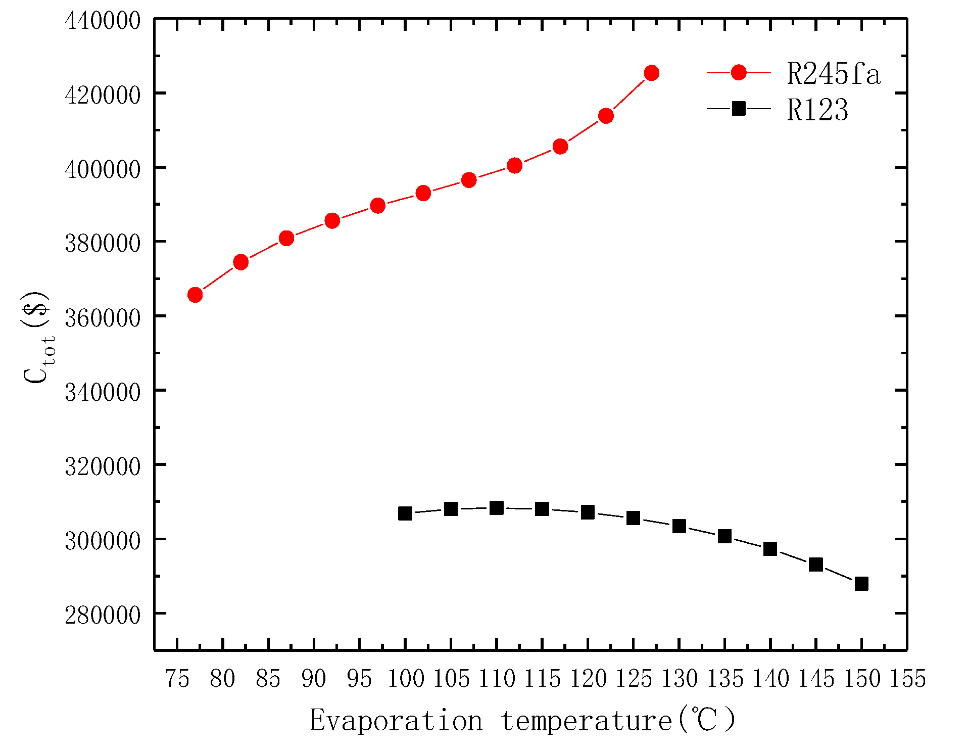
Figure 2 depicts the total cost of ORC system at different evaporation temperatures. In the figure, it can be seen that the total cost of ORC system with R123 as working fluid decreases with the increase of evaporation temperature, while, for the ORC system with R245fa as working fluid, its total cost increases. With the increase of evaporation temperature, as for the R123 system, its heat transfer area in evaporator decreases. The output power of expander increases first and then decreases. The heat transfer area in condenser decreases. The work consumed by pump increases. The investment reduction rate of the evaporator is greater than the increase rate of the expander investment, so the total investment of system decreases as a whole. As for R245fa system, the heat transfer areas in both evaporator and condenser decreases. Both the output power of expander and the work consumed by pump increases. The investment reduction rate of the evaporator is less than the increase rate of the expander investment, so the total investment increases as a whole.
Figure 3 depicts the net earnings (NE) of ORC system at different evaporation temperatures. In the figure, it can be seen that, with the increase of evaporation temperature, the net earnings (NE) of the R123 system increase first and then decreases, while, for the R245fa system, its net earnings (NE) increase. Multiplying the output power by the working fluid flow, the product obtained is sold in units of on-grid electricity price within one year. This income is the net earnings (NE) of ORC system. With the increase of evaporation temperature, the flow rate of R123 decreases while the output work increases. When the two items are multiplied, the net earnings (NE) of ORC system show a maximum at the evaporation temperature of 120 °C. As for the R245fa system, the reduction rate of mass flow rate of working fluid is less than the increase rate of output work of system, thus the net earnings (NE) of system increases.
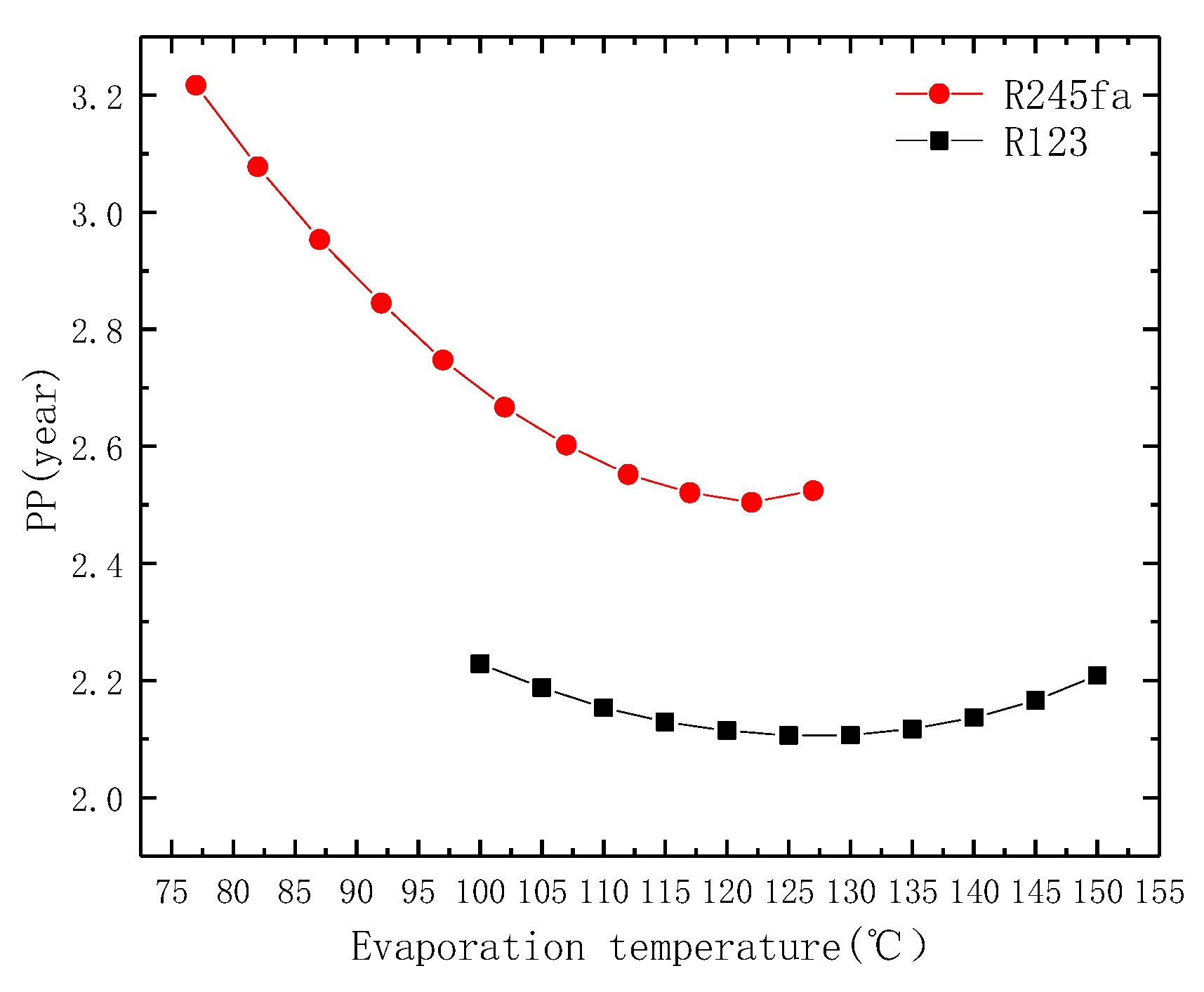
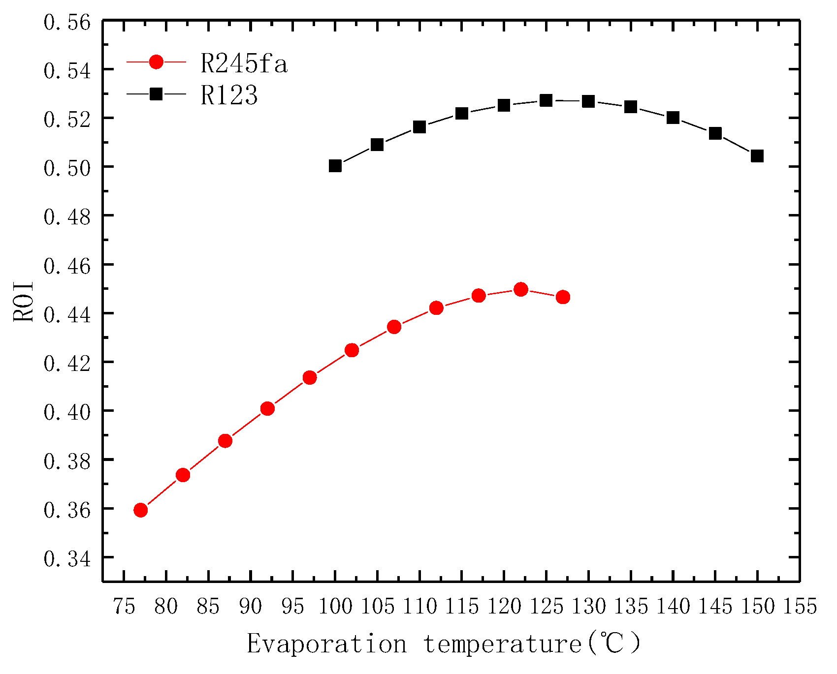
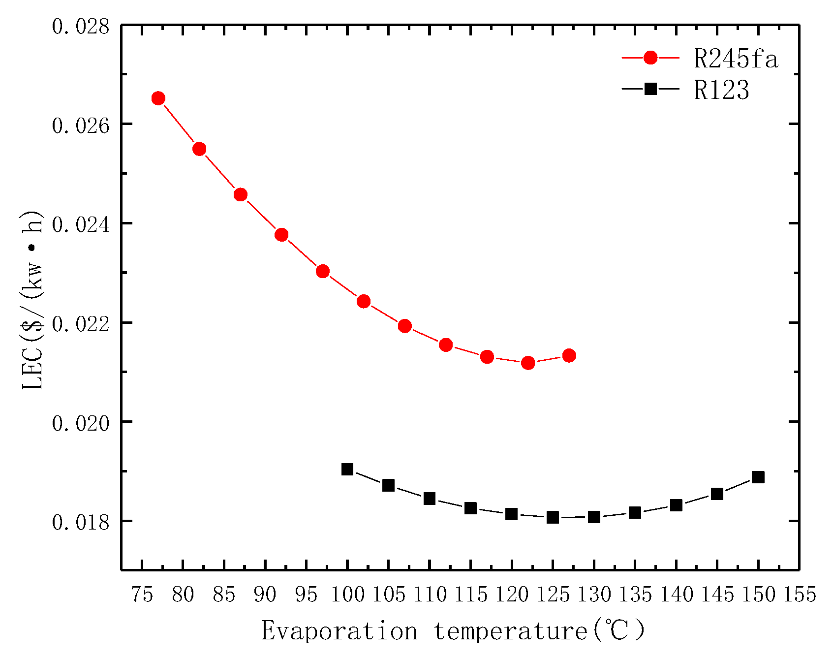
Figure 4, Figure 5 and Figure 6 depict the payback period (PP), return on investment (ROI), and levelized energy cost (LEC) of ORC system at different evaporation temperatures, respectively. In the figures, it can be seen that there is an optimal value for each of the above three indicators. For R123 system, the optimum evaporation temperature is 125 °C and it is 122 °C for R245fa system. All three indicators are based on the ratio of net earnings to total cost of system. Therefore, an optimal value appears when the above two indicators have different variation rates.
Present value of total profit in system service life of ORC system at different evaporation temperatures is depicted by Figure 7. In the figure, it can be seen that, for R123 system, there is an optimal value at the evaporation temperature of 120 °C, while, for R245fa system, the value increases with the increase of evaporation temperature. The present value of total profit in system service life of ORC system is related to two factors, total cost and net earnings of the system. The latter affects the value greatly. For the R123 system, the net earnings reach maximum at the evaporation temperature of 120 °C and the total cost of the system is small. Therefore, the present value of total profit in system service life has a maximum value at 120 °C. For R245fa system, its increase rate of net earnings is greater than that of total cost of the system. Therefore, its present value of total profit in system service life increases with the increase of evaporation temperature.
From the above discussion, it can be seen that, for R123 system, its payback period (PP), return on investment (ROI), and levelized energy cost (LEC) reach optimal at the evaporation temperature of 125 °C and its net earnings (NE) and present value of total profit in system service life have the optimal value at the evaporation temperature of 120 °C. Considering that the total cost of the system is relatively low when the evaporation temperature is 125 °C, this is the optimal evaporation temperature for R123 system.
As for R245fa system, its payback period (PP), return on investment (ROI), and levelized energy cost (LEC) reach optimal at the evaporation temperature of 122 °C. When above 122 °C, its growth rate of total cost of the system accelerates, while its growth rates of net earnings and present value of total profit in system service life slow down. Therefore, 122 °C is the optimal evaporation temperature for R245fa system.
3.2. Variation Effects of Condensation Temperature on Economic Performance of ORC System
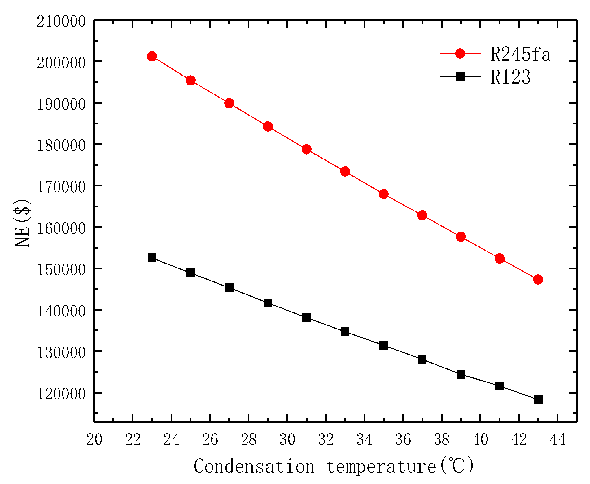
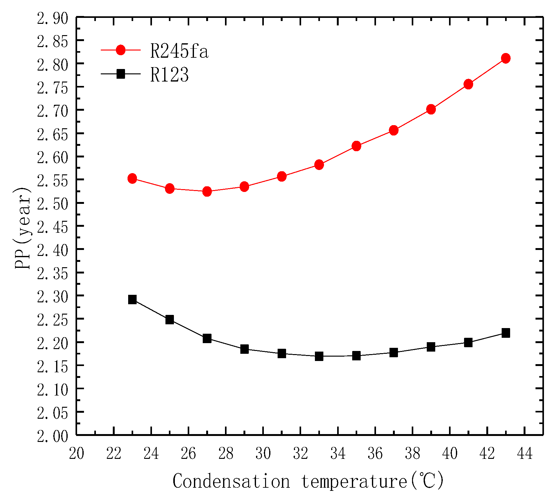
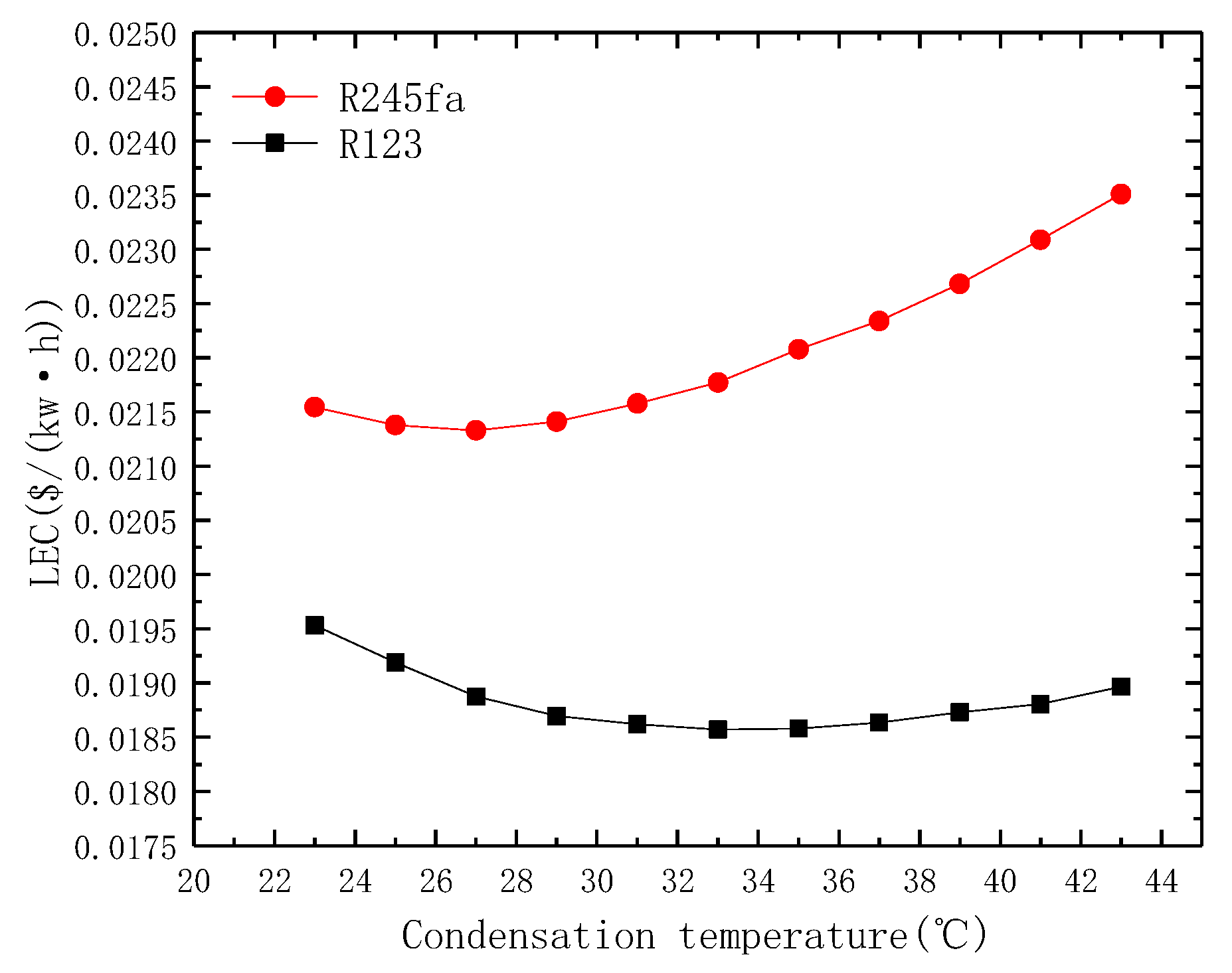
In this study, the evaporation temperature of R123 was set at 150 °C and 127 °C for R245fa. The condensation temperature was in the range of 23–43 °C. The heat source temperature was set at 197 °C Total cost, net earnings, payback period, return on investment, levelized energy cost, and present value of total profit in system service life of ORC system at different condensation temperatures are depicted in Figure 8, Figure 9, Figure 10, Figure 11, Figure 12 and Figure 13.
In these figures, it can be seen that, with the condensation temperature increase, there are three decreasing indicators: total cost, net earnings, and present value of total profit in system service life. With the increase of condensation temperature, the heat exchange in the condenser, the required heat transfer area, and the cost of condenser decrease, accordingly. Moreover, the output work of the system decreases and the cost of expander decreases. Therefore, both the total cost and net earnings of the system decrease. The net earnings of the system can greatly affect the present value of total profit in system service life, which also decreases accordingly. Three indicators, payback period (PP), return on investment (ROI), and levelized energy cost (LEC) of ORC system, which are based on the ratio of net earnings to total cost of system, have an optimal value of condensation temperature. R123 and R245fa systems have optimal condensation temperatures of 33 °C and 27 °C, respectively. In summary, when the above six indicators are considered, the optimal condensation temperature of R123 system is determined to be 33 °C and that of R245fa system is 27 °C.
3.3. Variation Effects of Heat Source Temperature on Economic Performance of ORC System
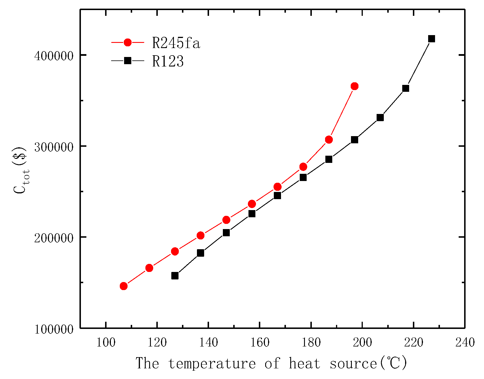
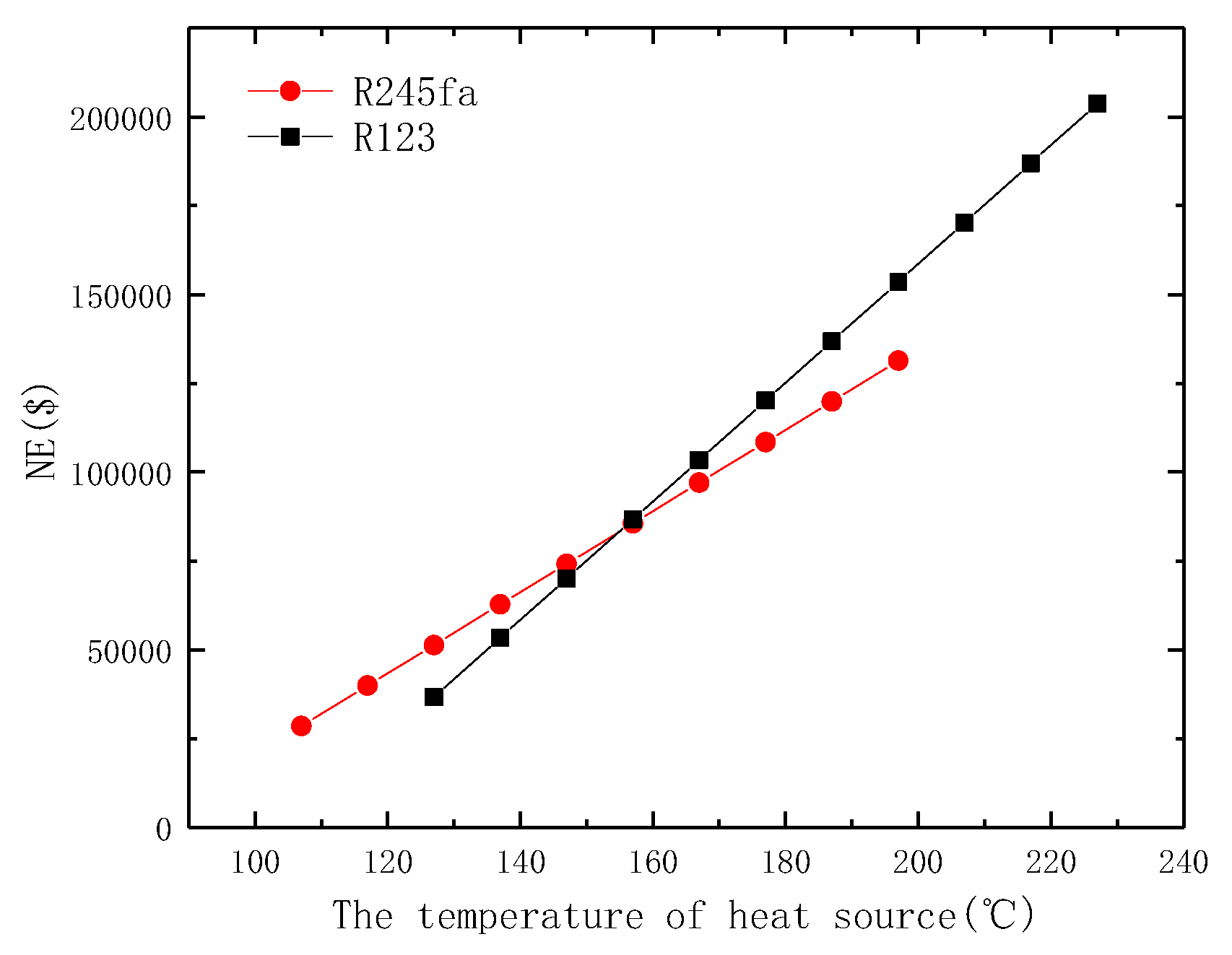
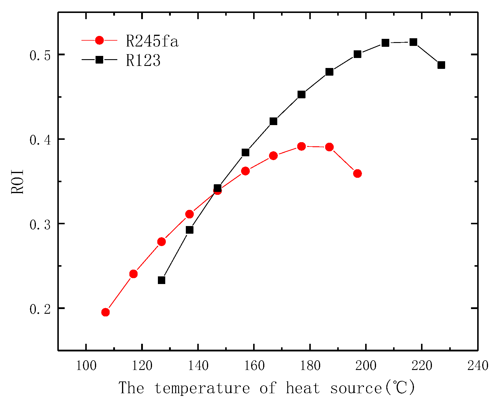
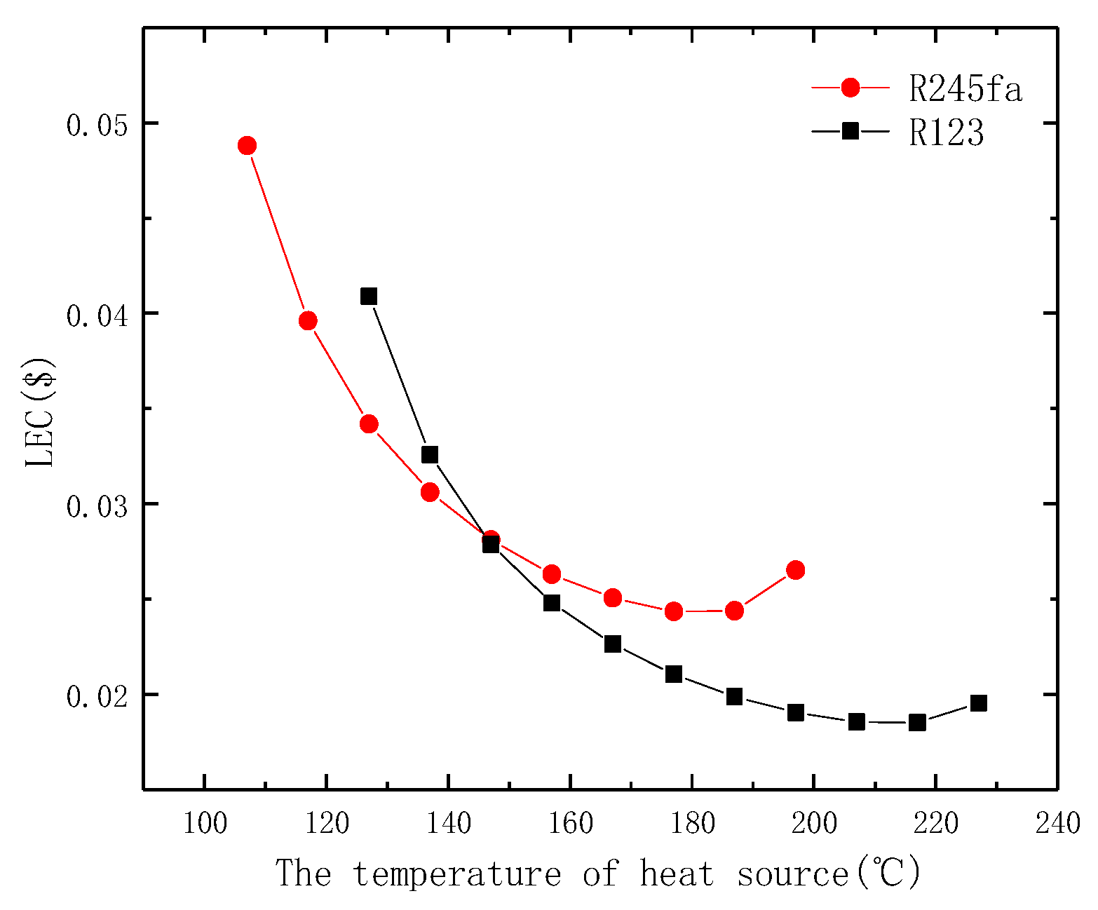
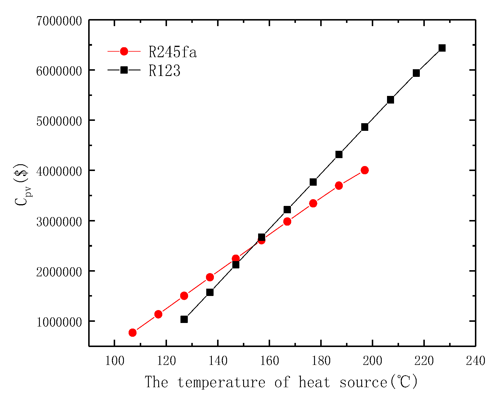
The flue gas is used as heat source. For R123 system, the heat source temperature was set in the range of 127–227 °C and that for R245fa system was 107–197 °C. The condensation temperature was set at 27 °C. Considering that the outlet temperature of heat source should not be lower than the inlet temperature of evaporator when pinch point temperature difference method is used, the above heat source temperatures were set. Total cost, net earnings, payback period, return on investment, levelized energy cost, and present value of total profit in system service life of ORC system at different heat source temperatures are depicted in Figure 14, Figure 15, Figure 16, Figure 17, Figure 18 and Figure 19.
In the above figures, it can be seen that, with the increase of heat source temperature, there are three increasing indicators: total cost, net earnings, and present value of total profit in system service life. With the increase of heat source temperature, the mass flow rate of working fluid increases. The required heat transfer areas in evaporator and condenser increase and their costs increase, accordingly. Both the output work of expander and the work consumed by pump increase and their costs increase, accordingly. Therefore, the total cost of system increases and its growth rate accelerates when the heat source temperature is above 217 °C (for R123 system) and 177 °C (for R245fa system). The net earnings of the system increases because of the increase of both the output work of the system and the mass flow rate of working fluid. The net earnings of the system can greatly affect the present value of total profit in system service life, which also increases, accordingly. Three indicators, payback period (PP), return on investment (ROI), and levelized energy cost (LEC) of ORC system, have an optimal value of heat source temperature. R123 and R245fa systems have optimal heat source temperatures of 217 °C and 177 °C, respectively. In summary, when the above six indicators are considered, the optimal heat source temperature of R123 system is determined to be 217 °C and that of R245fa system is 177 °C.
3.4. Variation Effects of Mass Flow Rate of Heat Source on Economic Performance of ORC System
To study the effect of mass flow rate of heat source on the economic performance of ORC system, for R123 system, the evaporation temperature was set at 150 °C, condensation temperature was set at 27 °C, and heat source temperature was set at 197 °C. For R245fa system, the evaporation temperature was set at 127 °C, condensation temperature was set at 27 °C, and heat source temperature was set at 197 °C. Total cost, net earnings, payback period, return on investment, levelized energy cost, and present value of total profit in system service life of ORC system with different mass flow rates of heat source are depicted in Figure 20, Figure 21, Figure 22, Figure 23, Figure 24 and Figure 25.
From the above figures, it can be seen that, with the increase of mass flow rate of heat source, although the total cost of the system increases, the net earnings, return on investment, and present value of total profit in system service life increase. Meanwhile, the payback period and levelized energy cost decrease. Therefore, the economic performance of system becomes better and better with the increase of mass flow rate of heat source.
4. A Demonstration Project Report
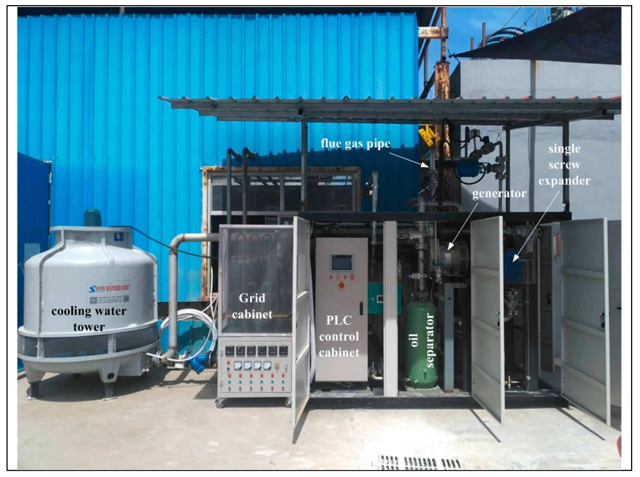
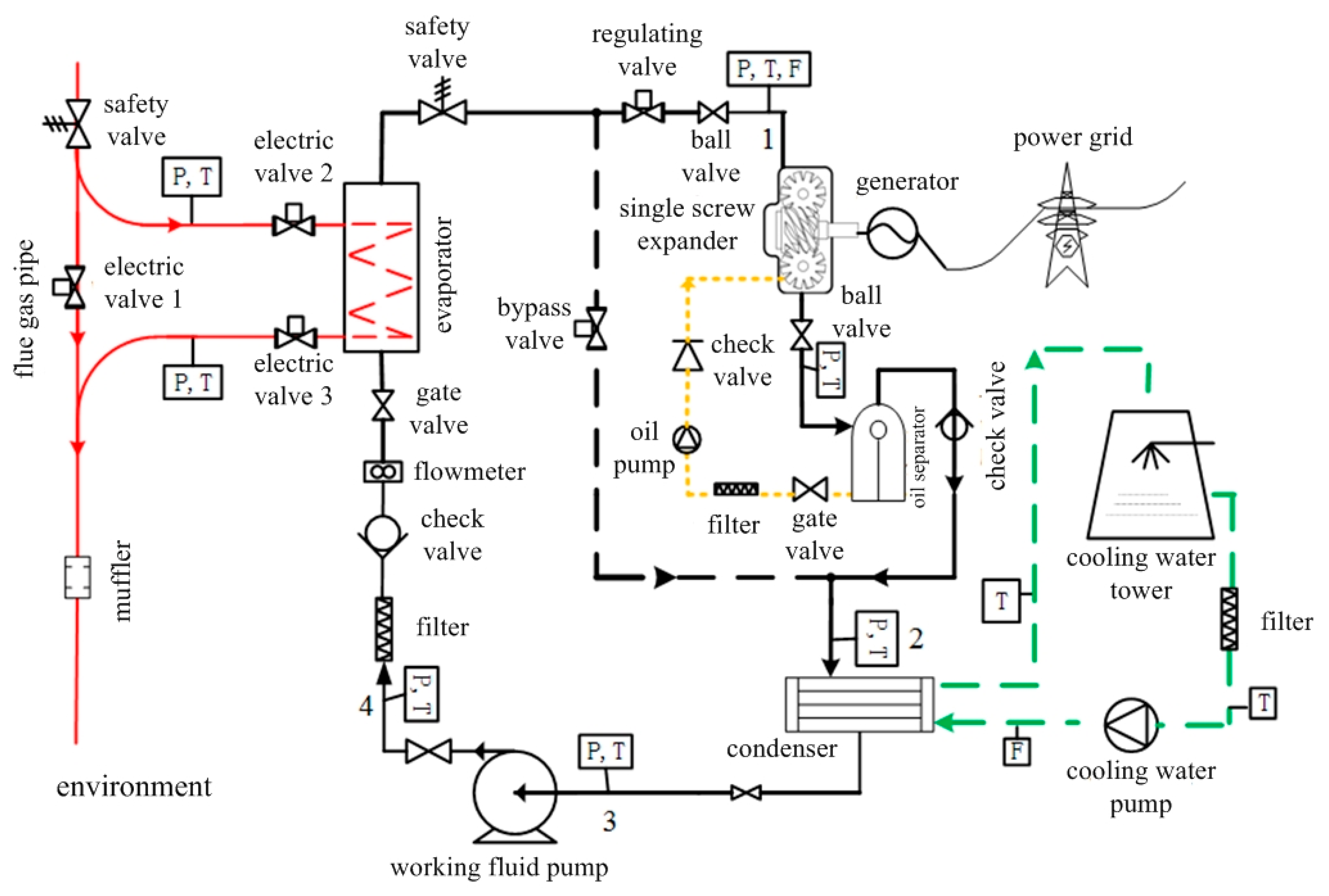
A demonstration project of ORC system with R123 as working fluid was established in Liulin, Shanxi province, P. R. China. This project is used for the waste heat recover of flue gas from a gas-fired internal combustion engine generator unit. Figure 26 presents a photograph of the ORC system demonstration project. Its scheme is depicted in Figure 27. The working condition parameters of the demonstration ORC system are listed in Table 5. Its output power is 11 kW.
The investment cost of the equipment used in the demonstration ORC system is listed in Table 6. Table 7 gives the value of economic indicators used to analyze the economic performance of demonstration ORC system.
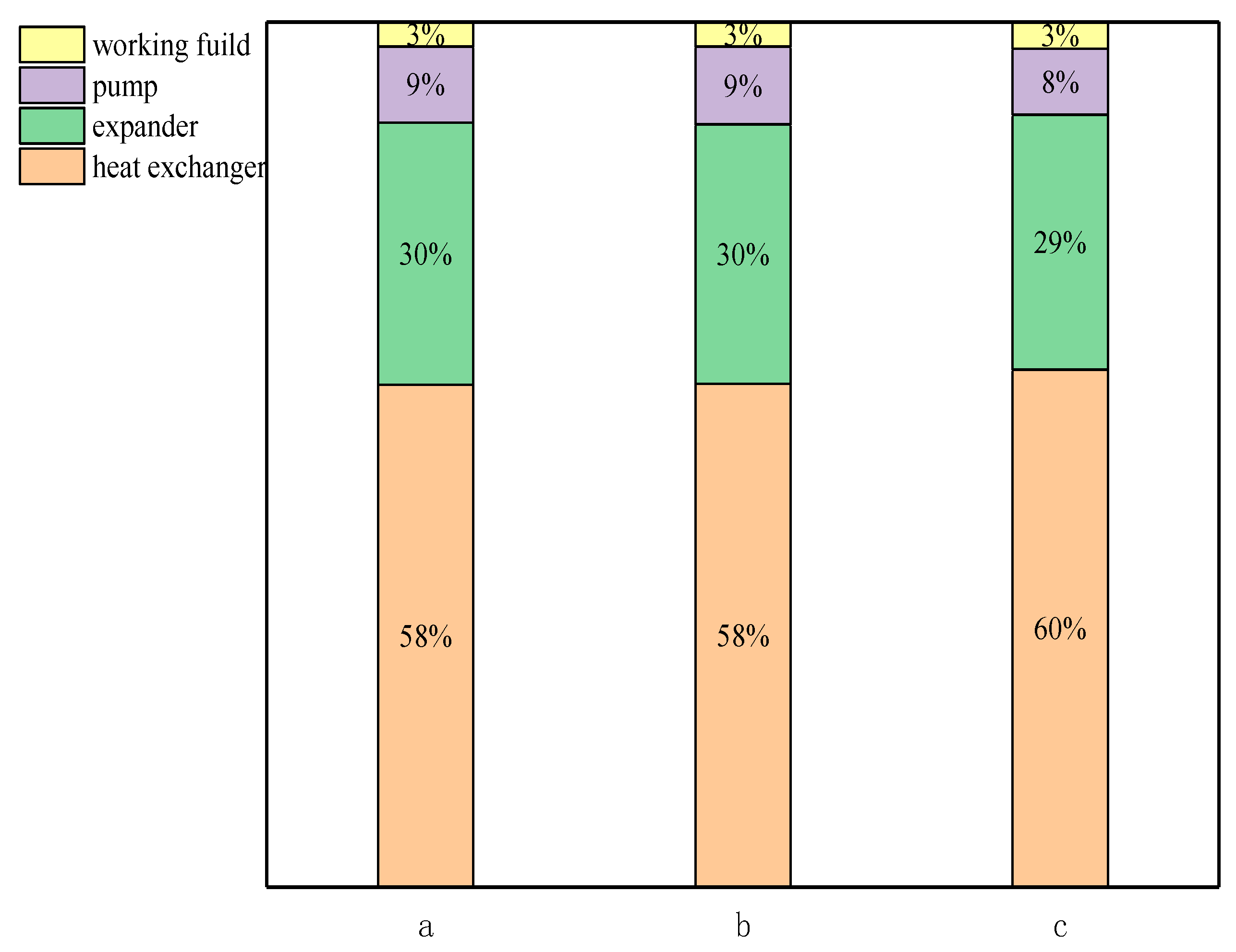
In the previous section, the calculation results show that the optimal evaporation temperature of R123 is 125 °C, optimal condensation temperature is 33 °C, and optimal heat source temperature is 217 °C. For R245fa, the optimal evaporation temperature is 122 °C, optimal condensation temperature is 27 °C, and optimal heat source temperature is 177 °C. Figure 28 depicts the proportion of equipment investment in the ORC system with R123 as working fluid at the optimal evaporation temperature, optimal condensation temperature, and optimal heat source temperature. The proportion of equipment investment in demonstration project is also depicted in Figure 28. The proportion of equipment investment in the ORC system with R245fa as working fluid at the optimal evaporation temperature, optimal condensation temperature, and optimal heat source temperature is depicted in Figure 29.
For R123 and R245fa systems, it was found that the investment in heat exchanger accounted for the largest proportion, followed by expander, then pump, and the least was the investment in working fluid. For the demonstration project, the investment in heat exchanger accounted for the largest proportion, followed by expander, working fluid accounts for the third, and the least was the investment in pump. This is because, as the key equipment in ORC system, the expander used in the demonstration project is a single screw expander, which was independently researched, developed and produced by our research group. Therefore, its cost was greatly reduced. Moreover, the previous calculation of the investment in working fluid was based on the total quantity that fills heat exchanger chamber and the system piping. In the demonstration project, the additional quantity of working fluid caused by leakage and loss should be considered. Therefore, in the demonstration project, the investment proportion of working fluid was higher than that of pump.
5. Conclusions
Considering traditional and classical indicators mainly focus on the present economic performance evaluation, a relatively new indicator, which is called present value of total profit in system service life, is proposed in this paper. Economic performance of ORC systems with R123 and R245fa as working fluid was analyzed using five traditional economic indicators (total cost, net earnings, payback period, return on investment, and levelized energy cost) and the relatively new indicator.
From the calculation results, the following conclusion can be drawn.
(1) Considering the variation effects of evaporation temperature on economic performance of ORC system, for R123 system, its payback period (PP), return on investment (ROI), and levelized energy cost (LEC) reach optimal at the evaporation temperature of 125 °C and its net earnings (NE) and present value of total profit in system service life have the optimal value at the evaporation temperature of 120 °C. Considering that the total cost of the system is relatively low when the evaporation temperature is 125 °C, this is the optimal evaporation temperature for R123 system. As for R245fa system, its payback period (PP), return on investment (ROI), and levelized energy cost (LEC) reach optimal at the evaporation temperature of 122 °C. When above 122 °C, its growth rate of total cost of the system accelerates, while its growth rates of net earnings and present value of total profit in system service life slow down. Therefore, 122 °C is the optimal evaporation temperature for R245fa system.
(2) Considering the variation effects of condensation temperature, three indicators, payback period (PP), return on investment (ROI), and levelized energy cost (LEC) of ORC system, which are based on the ratio of net earnings to total cost of system, have an optimal value of condensation temperature. R123 and R245fa systems have optimal condensation temperatures of 33 °C and 27 °C, respectively.
(3) Considering the variation effects of heat source temperature, with the increase of heat source temperature, there are three increasing indicators: total cost, net earnings, and present value of total profit in system service life. R123 and R245fa systems have optimal heat source temperatures of 217 °C and 177 °C, respectively.
(4) Considering the variation effects of mass flow rate of heat source, with the increase of mass flow rate of heat source, although the total cost of system increases, the net earnings, return on investment, and present value of total profit in system service life increase. Meanwhile, the payback period and levelized energy cost decrease. Therefore, the economic performance of system becomes better and better with the increase of mass flow rate of heat source.
(5) If the above four variation effects are considered comprehensively, the results show that the optimal evaporation temperature of R123 is 125 °C, optimal condensation temperature is 33 °C, and optimal heat source temperature is 217 °C. For R245fa, the optimal evaporation temperature is 122 °C, optimal condensation temperature is 27 °C, and optimal heat source temperature is 177 °C. The investment in heat exchanger accounted for the largest proportion, followed by expander, then pump, and the least was the investment in working fluid.
(6) The economic performance of an ORC demonstration project was reported. The investment in heat exchanger accounted for the largest proportion, followed by expander, working fluid accounts for the third, and the least was the investment in pump.
Author Contributions
Conceptualization, X.Z.; Data curation, M.C.; Formal analysis, M.C. and X.Y.; Funding acquisition, X.Z. and H.G.; Methodology, X.Z. and X.Y.; Writing—original draft, X.Z.; and Writing—review and editing, H.G. and J.W.
Funding
This research was funded by the National Natural Science Foundation of China (Grant No.51506001), Beijing Municipal Education Commission (Grant No. KM201710005029), and National Key R&D Program of China (Grant No. 2016YFE0124900). The authors gratefully acknowledge them for financial support of this work.
Conflicts of Interest
The authors declare no conflict of interest.
Nomenclature Symbol
| m | mass flow rate (kg/s) |
| cp | specific heat capacity at constant pressure (kJ/kg·K) |
| T | temperature (°C) |
| ΔT | pinch point temperature difference (°C) |
| h | enthalpy (kJ/kg) |
| d | internal diameter (mm) |
| D | external diameter (mm) |
| Re | Reynolds number |
| Pr | Prandtl number |
| Bo | boiling characteristic number |
| x | vapor quality |
| Q | heat (kW) |
| K | heat transfer coefficient (W/m2·K) |
| ΔTm | logarithmic mean temperature difference (K) |
| A | heat transfer area (m2) |
| W | work (kW) |
| p | pressure (MPa) |
| pw | price of working fluid ($/kg) |
| Mw | mass of working fluid (kg) |
| pe | price of electricity ($/kW·h) |
| ρ | density (kg/m3) |
| μ | dynamic viscosity (Pa·s) |
| δ | thickness of the tube (mm) |
| α | convective heat transfer coefficient (W/m2·K) |
| λ | thermal conductivity (W/m·K) |
| Subscripts | |
| 1–6 | state points in the cycle |
| g | flue gas |
| wf | working fluid |
| w | cooling water |
| i | inlet |
| o | outlet |
| l | liquid |
| v | vapor |
| e | evaporator |
| c | condenser |
| E | evaporation |
| C | condensation |
| min | minimum |
| max | maximum |
| s | single-phase |
| t | two-phase |
| ex | expander |
| p | pump |
| Abbreviation | |
| ORC | Organic Rankine Cycle |
| CEPCI | Chemical Engineering Plant Cost Index |
| NE | Net Earning |
| ROI | Return on Investment |
| COM | Cost of Maintenance |
| PP | Payback Period |
| LEC | Levelized Energy Cost |
| CPV | present value of total profile in system service life |
References
- Quoilin, S.; Declaye, S.; Tchanche, B.F.; Lemort, V. Thermo-economic optimization of waste heat recovery Organic Rankine Cycles. Appl. Therm. Eng. 2011, 31, 2885–2893. [Google Scholar] [CrossRef] [Green Version]
- Quoilin, S.; Lemort, V.; Lebrun, J. Experimental study and modeling of an Organic Rankine Cycle using scroll expander. Appl. Energy 2010, 87, 1260–1268. [Google Scholar] [CrossRef]
- Declaye, S.; Quoilin, S.; Guillaume, L.; Lemort, V. Experimental study on an open-drive scroll expander integrated into an ORC (Organic Rankine Cycle) system with R245fa as working fluid. Energy 2013, 55, 173–183. [Google Scholar] [CrossRef]
- Braimakis, K.; Karellas, S. Energetic optimization of regenerative Organic Rankine Cycle (ORC) configurations. Energy Convers. Manag. 2018, 159, 353–370. [Google Scholar] [CrossRef]
- Braimakis, K.; Karellas, S. Integrated thermoeconomic optimization of standard and regenerative ORC for different heat source types and capacities. Energy 2017, 121, 570–598. [Google Scholar] [CrossRef]
- Braimakis, K.; Karellas, S. Exergetic optimization of double stage Organic Rankine Cycle (ORC). Energy 2018, 149, 296–313. [Google Scholar] [CrossRef]
- Carraro, G.; Pallis, P.; Leontaritis, A.D.; Karellas, S.; Vourliotis, P.; Recha, S.; Lazzaretto, A. Experimental performance evaluation of a multi-diaphragm pump of a micro-ORC system. Energy Procedia 2017, 129, 1018–1025. [Google Scholar] [CrossRef]
- Heberle, F.; Preißinger, M.; Brüggemann, D. Zeotropic mixtures as working fluids in Organic Rankine Cycles for low-enthalpy geothermal resources. Renew. Energy 2012, 37, 364–370. [Google Scholar] [CrossRef]
- Preißinger, M.; Schatz, S.; Vogl, A.; König-Haagen, A.; Brüggemann, D. Thermoeconomic analysis of configuration methods for modular Organic Rankine Cycle units in low-temperature applications. Energy Convers. Manag. 2016, 127, 25–34. [Google Scholar] [CrossRef]
- Weiß, A.P.; Popp, T.; Müller, J.; Hauer, J.; Brüggemann, D.; Preißinger, M. Experimental characterization and comparison of an axial and a cantilever micro-turbine for small-scale Organic Rankine Cycle. Appl. Therm. Eng. 2018, 140, 235–244. [Google Scholar] [CrossRef]
- Shi, L.; Shu, G.; Tian, H.; Deng, S. A review of modified Organic Rankine cycles (ORCs) for internal combustion engine waste heat recovery (ICE-WHR). Renew. Sustain. Energy Rev. 2018, 92, 95–110. [Google Scholar] [CrossRef]
- Peris, B.; Navarro-Esbrí, J.; Molés, F. Bottoming organic Rankine cycle configurations to increase Internal Combustion Engines power output from cooling water waste heat recovery. Appl. Therm. Eng. 2013, 61, 364–371. [Google Scholar] [CrossRef] [Green Version]
- Seyedkavoosi, S.; Javan, S.; Kota, K. Exergy-based optimization of an organic Rankine cycle (ORC) for waste heat recovery from an internal combustion engine (ICE). Appl. Therm. Eng. 2017, 126, 447–457. [Google Scholar] [CrossRef]
- Tian, H.; Shu, G.; Wei, H.; Liang, X.; Liu, L. Fluids and parameters optimization for the organic Rankine cycles (ORCs) used in exhaust heat recovery of Internal Combustion Engine (ICE). Energy 2012, 47, 125–136. [Google Scholar] [CrossRef]
- Shu, G.; Liu, L.; Tian, H.; Wei, H.; Yu, G. Parametric and working fluid analysis of a dual-loop organic Rankine cycle (DORC) used in engine waste heat recovery. Appl. Energy 2014, 113, 1188–1198. [Google Scholar] [CrossRef]
- Sprouse, C., III; Depcik, C. Review of organic Rankine cycles for internal combustion engine exhaust waste heat recovery. Appl. Therm. Eng. 2013, 51, 711–722. [Google Scholar] [CrossRef]
- Karvonen, M.; Kapoor, R.; Uusitalo, A.; Ojanen, V. Technology competition in the internal combustion engine waste heat recovery: A patent landscape analysis. J. Clean. Prod. 2016, 112, 3735–3743. [Google Scholar] [CrossRef]
- Qiu, G.; Liu, H.; Riffat, S. Expanders for Micro-CHP Systems with Organic Rankine Cycle. Appl. Therm. Eng. 2011, 31, 3301–3307. [Google Scholar] [CrossRef]
- Tahir, M.M.; Yamada, N.; Hoshino, T. Efficiency of Compact Organic Rankine Cycle System with Rotary-Vane-Type Expander for Low-Temperature Waste Heat Recovery. Int. J. Mech. Mechatron. Eng. 2010. [Google Scholar] [CrossRef]
- Kolasi’nski, P.; Błasiak, P.; Rak, J. Experimental and Numerical Analyses on the Rotary Vane Expander Operating Conditions in a Micro Organic Rankine Cycle System. Energies 2016, 9, 606. [Google Scholar] [CrossRef]
- Gnutek, Z.; Kolasi’nski, P. The Application of Rotary Vane Expanders in Organic Rankine Cycle Systems—Thermodynamic Description and Experimental Results. J. Eng. Gas Turb. Power 2013, 135, 061901. [Google Scholar] [CrossRef]
- Bao, J.; Zhao, L. A Review of Working Fluid and Expander Selections for Organic Rankine Cycle. Renew. Sustain. Energy Rev. 2013, 24, 325–342. [Google Scholar] [CrossRef]
- Shao, L.; Zhu, J.; Meng, X.; Wei, X.; Ma, X. Experimental study of an organic Rankine cycle system with radial inflow turbine and R123. Appl. Therm. Eng. 2017, 124, 940–947. [Google Scholar] [CrossRef] [Green Version]
- Feng, Y.Q.; Hung, T.C.; He, Y.L.; Wang, Q.; Wang, S.; Li, B.X.; Lin, J.R.; Zhang, W. Operation characteristic and performance comparison of organic Rankine cycle (ORC) for low-grade waste heat using R245fa, R123 and their mixtures. Energy Convers. Manag. 2017, 144, 153–163. [Google Scholar] [CrossRef]
- Shu, G.; Zhao, M.; Tian, H.; Huo, Y.; Zhu, W. Experimental comparison of R123 and R245fa as working fluids for waste heat recovery from heavy-duty diesel engine. Energy 2016, 115, 756–769. [Google Scholar] [CrossRef]
- Pang, K.C.; Chen, S.C.; Hung, T.C.; Feng, Y.Q.; Yang, S.C.; Wong, K.W.; Lin, J.R. Experimental study on organic Rankine cycle utilizing R245fa, R123 and their mixtures to investigate the maximum power generation from low-grade heat. Energy 2017, 133, 636–651. [Google Scholar] [CrossRef]
- Sun, H.; Qin, J.; Yan, P.; Huang, H.; Hung, T.C. Performance evaluation of a partially admitted axial turbine using R245fa, R123 and their mixtures as working fluid for small-scale organic Rankine cycle. Energy Convers. Manag. 2018, 171, 925–935. [Google Scholar] [CrossRef]
- Feng, Y.Q.; Hung, T.C.; Wu, S.L.; Lin, C.H.; Li, B.X.; Huang, K.C.; Qin, J. Operation characteristic of a R123-based organic Rankine cycle depending on working fluid mass flow rates and heat source temperatures. Energy Convers. Manag. 2017, 131, 55–68. [Google Scholar] [CrossRef]
- Li, M.; Wang, J.; He, W.; Gao, L.; Wang, B.; Ma, S.; Dai, Y. Construction and preliminary test of a low-temperature regenerative Organic Rankine Cycle (ORC) using R123. Renew. Energy 2013, 57, 216–222. [Google Scholar] [CrossRef]
- Shu, G.; Zhao, J.; Tian, H.; Liang, X.; Wei, H. Parametric and exergetic analysis of waste heat recovery system based on thermoelectric generator and organic rankine cycle utilizing R123. Energy 2012, 45, 806–816. [Google Scholar] [CrossRef]
- Li, L.; Ge, Y.T.; Luo, X.; Tassou, S.A. Design and dynamic investigation of low-grade power generation systems with CO2 transcritical power cycles and R245fa organic Rankine cycles. Therm. Sci. Eng. Prog. 2018, 8, 211–222. [Google Scholar] [CrossRef]
- Li, L.; Ge, Y.T.; Luo, X.; Tassou, S.A. Experimental analysis and comparison between CO2 transcritical power cycles and R245fa organic Rankine cycles for low-grade heat power generations. Appl. Therm. Eng. 2018, 136, 708–717. [Google Scholar] [CrossRef]
- Luján, J.M.; Serrano, J.R.; Dolz, V.; Sánchez, J. Model of the expansion process for R245fa in an Organic Rankine Cycle (ORC). Appl. Therm. Eng. 2012, 40, 248–257. [Google Scholar] [CrossRef] [Green Version]
- Moradi, R.; Tascioni, R.; Habib, E.; Cioccolanti, L.; Villarini, M.; Bocci, E. Thermodynamic simulation of a small-scale organic Rankine cycle testing facility using R245fa. Energy Procedia 2018, 148, 66–73. [Google Scholar] [CrossRef]
- Tsatsaronis, G. Thermoeconomical Analysis of Energy Conversion Processes; Habilitation at RWTH Aachen: Aachen, Germany, 1983. (In German) [Google Scholar]
- Kim, S.M.; Oh, S.D.; Kwon, Y.H.; Kwak, H.Y. Exergoeconomic analysis of thermal systems. Energy 1998, 23, 393–406. [Google Scholar] [CrossRef]
- Lazzaretto, A.; Tsatsaronis, G. SPECO: A systematic and general methodology for calculating efficiencies and costs in thermal systems. Energy 2006, 31, 1257–1289. [Google Scholar] [CrossRef]
- Zhang, S.; Wang, H.; Guo, T. Performance comparison and parametric optimization of subcritical Organic Rankine Cycle (ORC) and transcritical power cycle system for low-temperature geothermal power generation. Appl. Energy 2011, 88, 2740–2754. [Google Scholar]
- Abusoglu, A.; Kanoglu, M. Exergoeconomic analysis and optimization of combined heat and power production: A review. Renew. Sustain. Energy Rev. 2009, 13, 2295–2308. [Google Scholar] [CrossRef]
- Vélez, F.; Segovia, J.J.; Martín, M.C.; Antolín, G.; Chejne, F.; Quijano, A. A technical, economical and market review of organic Rankine cycles for the conversion of low-grade heat for power generation. Renew. Sustain. Energy Rev. 2012, 16, 4175–4189. [Google Scholar] [CrossRef]
- Fiaschi, D.; Manfrida, G.; Rogai, E.; Talluri, L. Exergoeconomic analysis and comparison between ORC and Kalina cycles to exploit low and medium-high temperature heat from two different geothermal sites. Energy Convers. Manag. 2017, 154, 503–516. [Google Scholar] [CrossRef]
- Yari, M.; Mehr, A.S.; Zare, V.; Mahmoudi, S.M.S.; Rosen, M.A. Exergoeconomic comparison of TLC (trilateral Rankine cycle), ORC (organic Rankine cycle) and Kalina cycle using a low grade heat source. Energy 2015, 83, 712–722. [Google Scholar] [CrossRef]
- Meinel, D.; Wieland, C.; Spliethoff, H. Economic comparison of ORC (Organic Rankine cycle) processes at different scales. Energy 2014, 74, 694–706. [Google Scholar] [CrossRef]
- Esen, H.; Inalli, M.; Esen, M. A techno-economic comparison of ground-coupled and air-coupled heat pump system for space cooling. Build. Environ. 2007, 42, 1955–1965. [Google Scholar] [CrossRef]
- Varga, Z.; Csaba, T. Techno-economic evaluation of waste heat recovery by organic Rankine cycle using pure light hydrocarbons and their mixtures as working fluid in a crude oil refinery. Energy Convers. Manag. 2018, 174, 793–801. [Google Scholar] [CrossRef]
- Luo, X.; Liang, Z.; Guo, G.; Wang, C.; Chen, Y.; Ponce-Ortega, J.M.; El-Halwagi, M.M. Thermo-economic analysis and optimization of a zoetropic fluid organic Rankine cycle with liquid-vapor separation during condensation. Energy Convers. Manag. 2017, 148, 517–532. [Google Scholar] [CrossRef]
- Mago, P.J.; Chamra, L.M.; Somayaji, C. Performance analysis of different working fluids for use in organic Rankine cycles. Proc. Inst. Mech. Eng. Part A 2007, 221, 255–263. [Google Scholar] [CrossRef]
- Ammar, Y.; Joyce, S.; Norman, R.; Wang, Y.; Roskilly, A.P. Low grade thermal energy sources and uses from the process industry in the UK. Appl. Energy 2012, 89, 3–20. [Google Scholar] [CrossRef]
- Goortani, B.M.; Mateos-Espejel, E.; Moshkelani, M.; Paris, J. Energy efficiency improvement of a Kraft process through practical stack gases heat recovery. Appl. Therm. Eng. 2011, 31, 4091–4096. [Google Scholar] [CrossRef]
- Waste Heat Recovery: Technologies and Opportunities in U.S. Industry, Prepared by BCS, Incorporated March 2008. p. 8. Available online: https://www1.eere.energy.gov/manufacturing/intensiveprocesses/pdfs/waste_heat_recovery.pdf (accessed on 10 January 2019).
- Wang, D.; Ling, X.; Peng, H. Cost-effectiveness performance analysis of organic Rankine cycle for low grade heat utilization coupling with operation condition. Appl. Therm. Eng. 2013, 58, 571–584. [Google Scholar] [CrossRef]
- Gungor, K.E.; Winterton, R.H.S. Simplified general correlation for saturated flow boiling and comparisons of correlations with data. Chem. Eng. Res. Des. 1987, 65, 148–156. [Google Scholar]
- Shah, M.M. A general correlation for heat transfer during film condensation inside pipes. Int. J. Heat Mass Transf. 1979, 22, 547–556. [Google Scholar] [CrossRef]
- Turton, R.; Bailie, R.C.; Whiting, W.B.; Shaeiwitz, J.A. Analysis, Synthesis and Design of Chemical Processes, 4th ed.; Prentice Hall PTR: Upper Saddle River, NJ, USA, 2012. [Google Scholar]
Figure 1.
Typical process of an organic Rankine cycle (a dry fluid as working fluid).

Figure 2.
Total cost of ORC system at different evaporation temperatures.

Figure 3.
Net earnings (NE) of ORC system at different evaporation temperatures.

Figure 4.
Payback Period (PP) of ORC system at different evaporation temperatures.

Figure 5.
Return on Investment (ROI) of ORC system at different evaporation temperatures.

Figure 6.
Levelized Energy Cost (LEC) of ORC system at different evaporation temperatures.

Figure 7.
Present Value of Total Profit in System Service Life of ORC system at different evaporation temperatures.
Figure 7.
Present Value of Total Profit in System Service Life of ORC system at different evaporation temperatures.

Figure 8.
Total cost of ORC system at different condensation temperatures.

Figure 9.
Net earnings (NE) of ORC system at different condensation temperatures.

Figure 10.
Payback Period (PP) of ORC system at different condensation temperatures.

Figure 11.
Return on Investment (ROI) of ORC system at different condensation temperatures.

Figure 12.
Levelized Energy Cost (LEC) of ORC system at different condensation temperatures.

Figure 13.
Present Value of Total Profit in System Service Life of ORC system at different condensation temperatures.
Figure 13.
Present Value of Total Profit in System Service Life of ORC system at different condensation temperatures.

Figure 14.
Total cost of ORC system at different heat source temperatures.

Figure 15.
Net earnings (NE) of ORC system at different heat source temperatures.

Figure 16.
Payback Period (PP) of ORC system at different heat source temperatures.

Figure 17.
Return on Investment (ROI) of ORC system at different heat source temperatures.

Figure 18.
Levelized Energy Cost (LEC) of ORC system at different heat source temperatures.

Figure 19.
Present Value of Total Profit in System Service Life of ORC system at different heat source temperatures.
Figure 19.
Present Value of Total Profit in System Service Life of ORC system at different heat source temperatures.

Figure 20.
Total cost of ORC system with different mass flow rates of heat source.

Figure 21.
Net earnings (NE) of ORC system with different mass flow rates of heat source.

Figure 22.
Payback Period (PP) of ORC system with different mass flow rates of heat source.

Figure 23.
Return on Investment (ROI) of ORC system with different mass flow rates of heat source.

Figure 24.
Levelized Energy Cost (LEC) of ORC system with different mass flow rates of heat source.

Figure 25.
Present Value of Total Profit in System Service Life of ORC system with different mass flow rates of heat source.
Figure 25.
Present Value of Total Profit in System Service Life of ORC system with different mass flow rates of heat source.

Figure 26.
Demonstration project of ORC system used for the waste heat recovery of flue gas from a gas-fired internal combustion engine generator unit.
Figure 26.
Demonstration project of ORC system used for the waste heat recovery of flue gas from a gas-fired internal combustion engine generator unit.

Figure 27.
Scheme of the demonstration project of ORC system.

Figure 28.
Proportion of equipment investment in the ORC system with R123 as working fluid at: (a) optimal evaporation temperature; (b) optimal condensation temperature; (c) optimal heat source temperature; and (d) demonstration project.
Figure 28.
Proportion of equipment investment in the ORC system with R123 as working fluid at: (a) optimal evaporation temperature; (b) optimal condensation temperature; (c) optimal heat source temperature; and (d) demonstration project.

Figure 29.
Proportion of equipment investment in the ORC system with R245fa as working fluid at: (a) optimal evaporation temperature; (b) optimal condensation temperature; and (c) optimal heat source temperature.
Figure 29.
Proportion of equipment investment in the ORC system with R245fa as working fluid at: (a) optimal evaporation temperature; (b) optimal condensation temperature; and (c) optimal heat source temperature.


Table 1.
Typical waste heat temperature at low-medium temperature range from various sources.
| Type of Heat Source | Temperature (°C) |
|---|---|
| Steel Industry | 190–400 [48] |
| Glass Industry | 140–200 [48] |
| Chemical Industry | 230–340 [48] |
| Kraft Pulping Mill | 164–238 [49] |
| Steam Boiler Exhaust | 230–480 [50] |
| Gas Turbine Exhaust | 370–540 [50] |
| Reciprocating Engine Exhaust | 320–590 [50] |
| Heat treating furnace | 430–650 [50] |
| Drying and baking ovens | 230–590 [50] |
| Exhaust Gases Exiting Recovery Devices in Gasfired Boilers, Ethylene Furnaces, etc. | 70–230 [50] |
| Drying, Baking, and Curing Ovens | 90–230 [50] |
Table 2.
Parameter settings for thermodynamic calculation.
| Parameter | Value |
|---|---|
| Mass flow of heat source (kg/s) | 10 [51] |
| Cooling water temperature (°C) | 15 |
| Type of heat exchanger | tube-in-tube heat exchanger |
| Inner tube diameter of heat exchanger, d (mm) | 30 |
| Outer tube diameter of heat exchanger, D (mm) | 60 |
| Tube thickness of heat exchanger, δ (mm) | 1 |
| Heat exchanger material | Steel |
| Pinch temperature difference in heat exchanger (°C) | 5 |
Table 3.
Correction factors for purchased cost of heat exchanger [54].
Table 3.
Correction factors for purchased cost of heat exchanger [54].
| Correction Factors | Value | Correction Factors | Value |
|---|---|---|---|
| K1 | 3.2138 | B1 | 1.8 |
| K2 | 0.2688 | B2 | 1.5 |
| K3 | 0.0796 | FM | 1.25 |
| C1 | −0.0650 | CEPCI1996 | 382 |
| C2 | 0.0503 | CEPCI2016 | 606 |
| C3 | 0.0147 |
Table 4.
Correction factors for purchased cost of pump and expander [54].
Table 4.
Correction factors for purchased cost of pump and expander [54].
| Correction Factors | Value for Pump | Value for Expander |
|---|---|---|
| K1 | 3.4771 | 2.2476 |
| K2 | 0.135 | 1.4965 |
| K3 | 0.1438 | −0.1618 |
| C1 | −0.245832 | 0 |
| C2 | 0.259016 | 0 |
| C3 | −0.01363 | 0 |
| B1 | 1.89 | 0 |
| B2 | 1.35 | 0 |
| FM | 1.4 | 0 |
| CEPCI1996 | 382 | 382 |
| CEPCI2016 | 606 | 606 |
Table 5.
Working condition parameters of the demonstration ORC system.
| Working Condition Parameter | Value |
|---|---|
| Heat source temperature (°C) | 330–450 |
| Mass flow rate of flue gas (heat source) (kg/h) | 1700 |
| Type of evaporator | shell-and-tube heat exchanger |
| Evaporation temperature (°C) | 108–118 |
| Type of condenser | tube-in-tube heat exchanger |
| Condensation temperature (°C) | 30 |
| Cooling water temperature (°C) | 20 |
Table 6.
Investment of each equipment used in demonstration ORC system.
| Equipment | Price (¥/$) |
|---|---|
| Plate heat exchanger used for preheating | 4000/576 |
| Evaporator | 58,000/8357 |
| Condenser | 23,000/3314 |
| Cooling tower | 5400/778 |
| Single screw expander | 25,000/3602 |
| Circulating pump for working fluid | 9352/1348 |
| Working fluid, R123 | 17,000/2450 |
Table 7.
Economic indicator of the demonstration ORC system.
| Economic Indicator | Value |
|---|---|
| Total Cost ($) | 20,470 |
| Net Earnings (NE) ($) | 8800 |
| Return on Investment (ROI) (%) | 42.98 |
| Payback Period (PP) (Year) | 2.63 |
| Levelized Energy Cost (LEC) ($/kw·h) | 0.0222 |
| Present Value of Total Profit in System Service Life ($) | 274,398 |
© 2019 by the authors. Licensee MDPI, Basel, Switzerland. This article is an open access article distributed under the terms and conditions of the Creative Commons Attribution (CC BY) license (http://creativecommons.org/licenses/by/4.0/).
Share and Cite
MDPI and ACS Style
Zhang, X.; Cao, M.; Yang, X.; Guo, H.; Wang, J. Economic Analysis of Organic Rankine Cycle Using R123 and R245fa as Working Fluids and a Demonstration Project Report. Appl. Sci. 2019, 9, 288. https://doi.org/10.3390/app9020288
AMA Style
Zhang X, Cao M, Yang X, Guo H, Wang J. Economic Analysis of Organic Rankine Cycle Using R123 and R245fa as Working Fluids and a Demonstration Project Report. Applied Sciences. 2019; 9(2):288. https://doi.org/10.3390/app9020288
Chicago/Turabian StyleZhang, Xinxin, Min Cao, Xiaoyu Yang, Hang Guo, and Jingfu Wang. 2019. "Economic Analysis of Organic Rankine Cycle Using R123 and R245fa as Working Fluids and a Demonstration Project Report" Applied Sciences 9, no. 2: 288. https://doi.org/10.3390/app9020288
Note that from the first issue of 2016, this journal uses article numbers instead of page numbers. See further details here.