An Experimental Study of a Data Compression Technology-Based Intelligent Data Acquisition (IDAQ) System for Structural Health Monitoring of a Long-Span Bridge

Abstract

There has recently been an increase in interest in structural health monitoring (SHM) using wireless sensor networks. For SHM, in particular, it is important to accurately and efficiently measure the dynamic acceleration response using wireless sensor networks in real-time. For the purpose, a CAFB (cochlea-inspired artificial filter bank) has been developed in a previous study, which is a dynamic data compression technology. Since the developed CAFB can select and compress only the interested range of frequency signals from an entire response of a structure, it efficiently provides a real-time dynamic response based on wireless networking. CAFB of the previous study is optimized to selectively acquire low-frequency signals of sub-10 Hz, which is required for SHM of long and large-scale structures. According to the CAFB’s optimization using an El-Centro seismic waveform, six band-pass filters, 1.0 Hz interval, and 0.6 Hz bandwidth have been adapted. This article is to evaluate dynamic acceleration response performance of civil structures using the CAFB developed in the previous study. To achieve the purpose, the optimally-designed CAFB was embedded in an intelligent data acquisition (IDAQ) system. To evaluate the performance of the IDAQ system with the embedded CAFB, the real-time dynamic response was investigated for a model cable-stayed bridge, measured by a wire-measuring system and the CAFB-based IDAQ system simultaneously. The results show excellent agreement between the compressed dynamic response acquired by the CAFB-based IDAQ system and that acquired by the wire measuring system. In addition, the measurement from the CAFB-based IDAQ system revealed the modal information of the model bridge. The developed CAFB can determine and reconstruct the entire dynamic response from compression with modal information only; its efficient operation illustrates its potential to be utilized in real-time structural health monitoring.

1. Introduction

Civil structures are constantly affected by diverse forms of external forces and environmental influences during their life-time. The potential for error or oversight in their initial design and construction, negligence of the user, or other factors cannot be excluded from discussions regarding the structure’s long-term stability and safety and, therefore, to prevent large-scale damage or accidents, systematic management plans and countermeasures should be prepared in advance. As a part of such efforts, research into structural health monitoring (SHM) systems was begun earnestly by the construction field in the 1990s to evaluate the condition and detect damage to civil structures in real-time. Major large bridges are a key focus of the application efforts of SHM [1,2,3,4,5,6].

Currently, since existing SHM systems build upon existing wired measuring systems, it is expensive to expand the measuring channels and maintain and manage the very large response data sets obtained. Since long-term measurement is required for accurate SHM, new systems should outclass existing systems. Recently, measurement and monitoring technologies using wireless sensor networks (WSNs) have attracted attention [7,8,9,10], and application examples using WSNs in various fields have also been introduced [11,12,13,14,15,16,17,18]. In the construction field, Spencer et al. [19] and Lynch et al. [20] developed a smart SHM (S-SHM), in which WSNs are newly incorporated into SHM systems. For these systems, the cost of building the system is reduced and the CPU and memory are embedded in the sensor, so that by RF networking, simple preprocessing of the measured signal is possible. It is feasible to install the sensor in limited-access or dangerous environments not accessible by existing wired measuring systems. Nagayama et al. [21] and Rice et al. [22] developed the Imote2, a wireless sensor node that uses the concepts of S-SHM, and performed substantial research, including health monitoring and structural evaluation, on a full-scale bridge. Kurata et al. [23] developed another wireless sensor node, Narada, by adapting a self-recharging method using solar panels and an inter-sensor node sub-networking scheme to obtain more stable data compared to existing S-SHM systems, applying the node to the Carquinez Bridge in California, USA. In these studies, the S-SHM systems configured using individual wireless sensor nodes improve the economic feasibility of installation and obtain better efficiency in terms of the system configuration, operation, and management, compared to existing wire-based SHM systems [24].

It is highly important for SHM of civil structures to be able to measure an accurate dynamic acceleration response of the structure in real-time. Generally, since the measurement of the dynamic response of a structure requires a large amount of data via each channel compared to a simple static response, building and managing systems that can capture and analyze these data can vastly increase costs. The S-SHM systems previously developed, which use wireless sensor nodes, are limited in their performance once the number of input channels is increased, due to the significant increase in the data acquisition rate and the corresponding necessary storage capacity [20,22]. Optimum performance can be obtained by configuring the wireless sensor node at the level of a high-performance PC to improve the data processing speed and storage capacity. Furthermore, although diverse wireless communication methods (e.g., Bluetooth, Zigbee, Wi-Fi) are currently used, each one of them has weaknesses and strengths with respect to factors such as the limits of their communication distance, speed, and the number of expanded channels. However, if the initial volume of the raw data from the structure can be reduced, these fundamental limitations of existing wireless communication technologies can be overcome. To suitably realize WSN-based SHM for real-time applications, data compression technology is required to acquire and transmit the dynamic response efficiently, together with the performance improvement of the sensor node to the level of a high-performance PC to record and store the dynamic response of the civil structure stably.

Recently, Peckens et al. [25,26] developed a wireless sensor node using an analog filter bank by several neuron boards, and performed a real-time response test in a model structure. The studies show that since the CPU and wireless sensor nodes are designed specifically for the lab, thus being inevitably limited in performance and capacity, exact data acquisition will require an increment of the sampling rate or an expansion of the measurement channels. When the amount of data becomes larger, their performance becomes limited. Furthermore, although the performance of the neuron boards used for the analog filter bank was tested by performing a response experiment, the neuron board would need to be re-designed, re-built, and re-tested because of the changes in the measurement targets for the civil structure. Therefore, flexible and efficient SHM is limited by the practicality and usability of hardware-type neuron boards for realizing the analog filter bank.

In this context, the previous study [1,27] developed a CAFB (cochlea-inspired artificial filter bank), which is a dynamic data compression technology using the D-S/W-D (digital-software-design) method. A CAFB is a digital filter bank which consists of n number of band-pass filters to select and compress only interesting ranges of frequency signals from an entire response of a structure. A previous study optimized the CAFB using an El-Centro seismic waveform to selectively acquire raw signals of under 10 Hz, which is required for SHM on long and large-scale civil structures. The CAFB optimized for the El-Centro seismic waveform was designed with six filters, a spacing of 1.0 Hz, and a bandwidth of 0.6 Hz [27]. Then, by executing a numerical study on CAFB, its validity as a dynamic data compression technology has been proven.

This study, using CAFB optimized in the previous study [27], is to experimentally evaluate the dynamic acceleration response performance of civil structures. To do that, an intelligent data acquisition (IDAQ) system was developed based on digital software design by embedding the previously-developed CAFB into the wireless sensing system. For the IDAQ system developed here, the modal test was performed by application to a model cable-stayed bridge; the dynamic characteristics were analyzed from the acquired dynamic response. Furthermore, the result was evaluated in conjunction with the result of the wire measurement. The results show that the CAFB-based wireless sensing system realized in this study has excellent performance and stability compared to wired sensing systems. Additionally, the CAFB was effective in determining the accurate, compressed structural response around the frequency band of interest.

2. A Cochlea-Inspired Artificial Filter Bank (CAFB) for Structural Health Monitoring

2.1. Principle of the CAFB

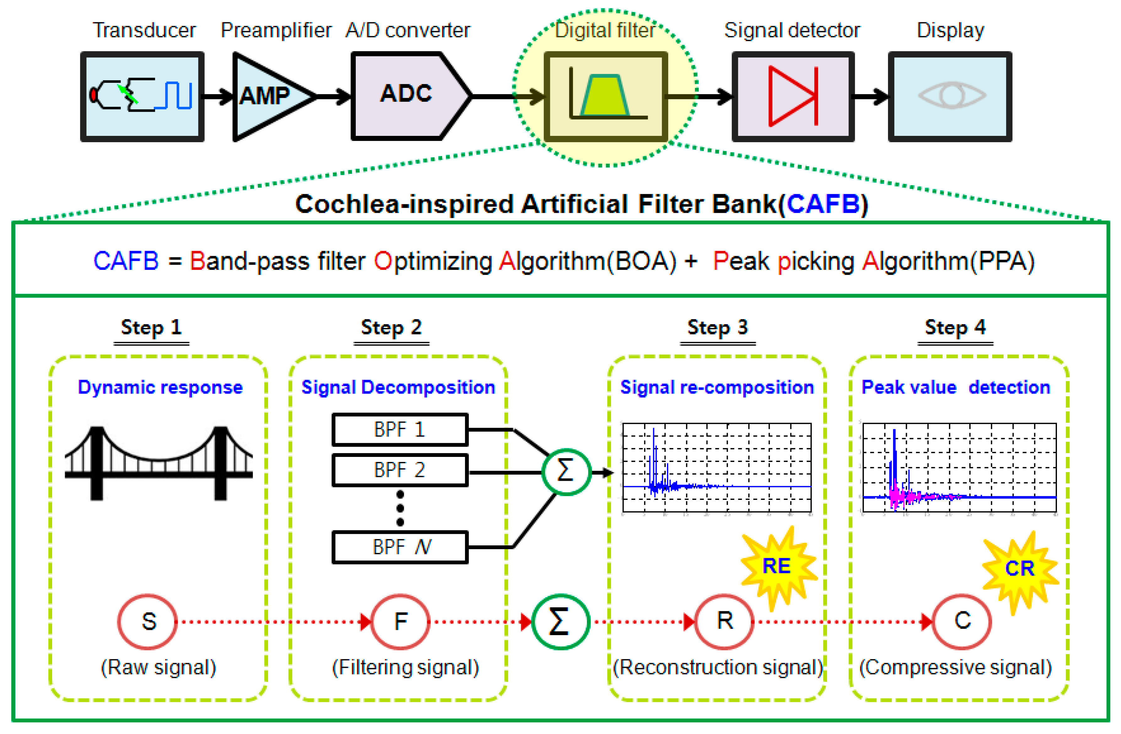
A previous study has developed the CAFB using n number of band-pass filters to obtain and compress the dynamic response for structures which is required in SHM on civil structures. As shown in Figure 1, CAFB is performed the signal processing (Input of signal (Step 1); Decomposition (Step 2); Reconstruction (Step 3); Compression (Step 4)) using a raw signal obtained from the structure.

As shown in Figure 1, CAFB is using two kinds of algorithms; one is BOA (band-pass optimizing algorithm) to selectively obtain the interested frequency band, and the other is PPA (peak picking algorithm) to compress the selected signals.

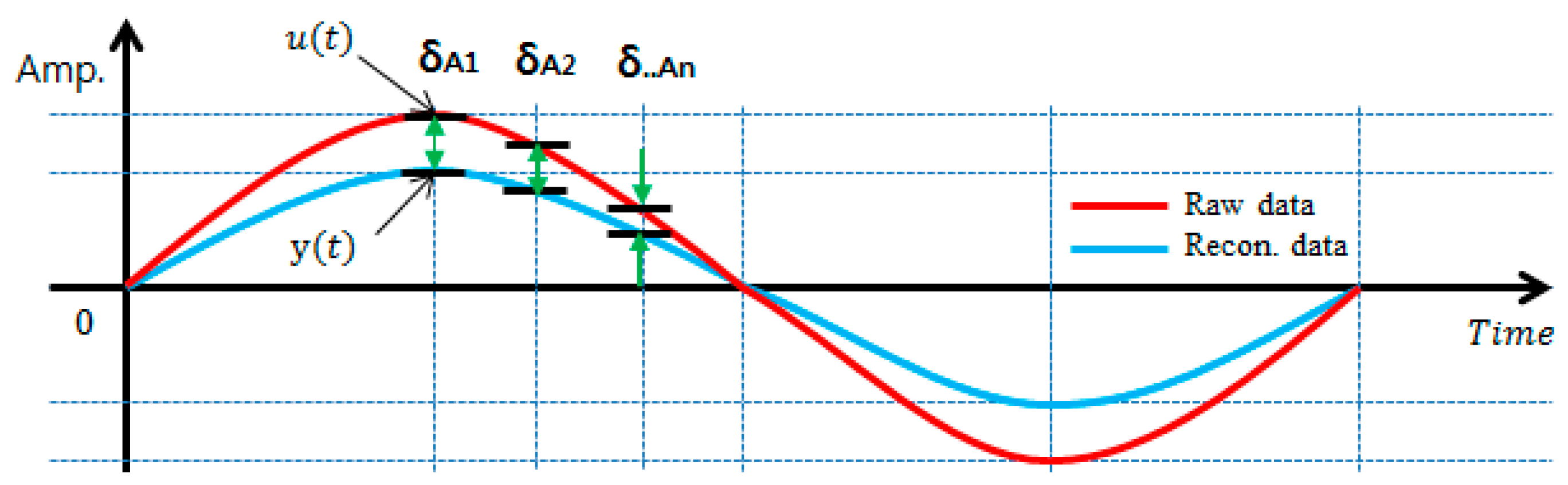
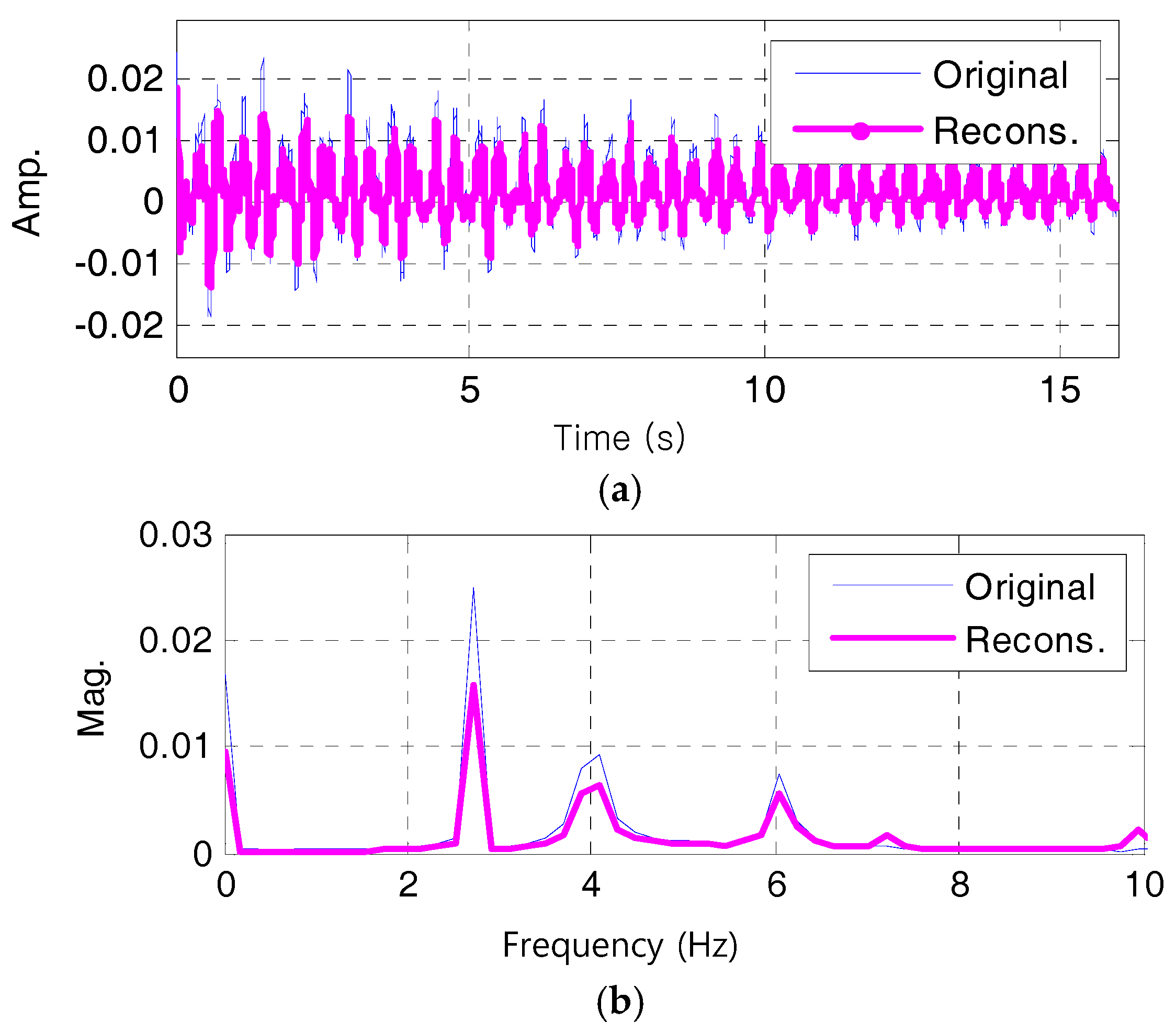
First, the BOA was used to design multiple band-pass filters in parallel such that they could be suitably used to determine the target mode required to evaluate the dynamic behavior of the civil structure and additionally calculate the reconstruction signal by altering the design conditions, such as the number, bandwidth, and interval of the band-pass filters. Finally, the reconstruction signal was evaluated through a comparison with the raw data acquired from the target structure. To evaluate the reconstruction signal compared to the raw data, the reconstruction error (RE) is the comparative difference between the composition of filtered signals and the original (raw) signal as expressed in Equation (1) and Figure 2. The RE defined in Equation (1) is represented by the relative difference of absolute values between the original and reconstruction signals. Here, u(t) is the raw data as a function of the response time, y(t) is the reconstruction signal as a function of the response time, and T is the total length of the response time, i.e., the total length of the input signal. The closer to 0 the reconstruction error is, the better the reconstruction effect.

$$\mathrm{RE}=\frac{{{\displaystyle \int }}_0^T\left|u\left(t\right)-y\left(t\right)\right|/\left|u\left(t\right)\right|}{T}=\frac{{{\displaystyle \int }}_0^T\left|{\delta }_i\right|/\left|u\left(t\right)\right|}{T}$$

(1)

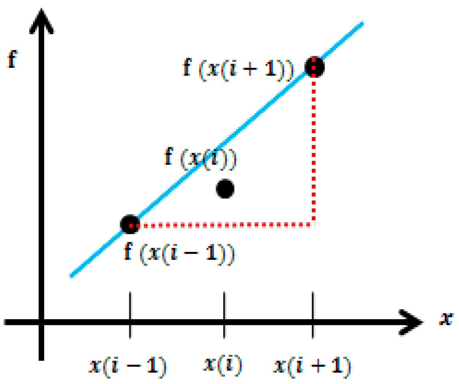
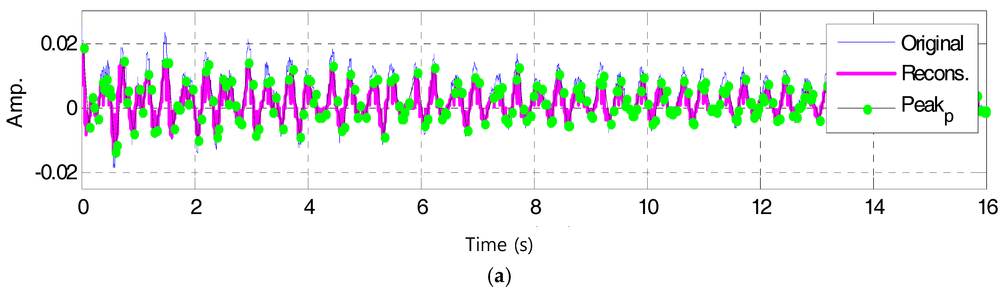
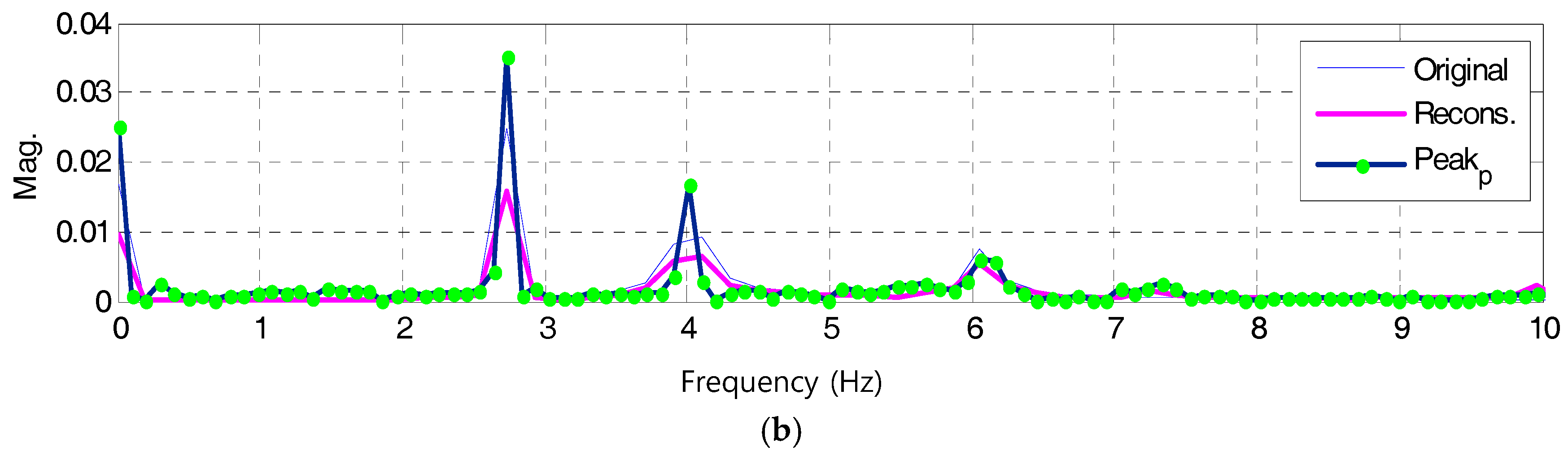
Next, a peak-picking algorithm (PPA) was developed for compression, which determines the peak value based on only the reconstruction signal determined through Equation (1). The PPA’s calculation process can be summarized as follows: First, the calculated reconstruction signal is read from the optimized filter bank. Second, the reconstruction signal is classified into three (3) data groups. Third, each group’s derived function is calculated based on three data points in each group. Fourth, peak values (time and measuring data) are derived by assessing the slope (sign) of each group’s derived function. In this study, a central difference method is used as a way to extract peak values while the PPA is calculating. Figure 3 below reveals the central difference method’s conceptual diagram, and a derived function can be calculated through Equation (2):

$$f^{\prime }\left(x\left(i\right)\right)=\frac{f\left(x\left(i+1\right)\right)-f\left(x\left(i-1\right)\right)}{x\left(i+1\right)-x\left(i-1\right)}$$

(2)

Based on the size of the reconstruction data determined through Equation (1) above, the effects of data compression through PPA can be defined by comparing a relative data size with the extracted peak value. For this, this study defines the data CR (compressive ratio) as stated in Equation (3) below:

$$\mathrm{CR}=\frac{N{S}_0-N{S}_C}{N{S}_0}$$

(3)

Here, $N{S}_C$ is the number of the compressive signal and $N{S}_{\mathrm{O}}$ is the number of the reconstruction signal. The closer to 0 the compressive ratio is, the better the compression effect is. The compressed signal is transmitted to the host through the WSNs.

The reconstruction error (RE) shown in Equation (1) signifies an index for the precision of reconstruction signals which were first filtered through the CAFB. Especially, it is one of the optimization elements along with the CR in Equation (3) which is used to calculate the optimal conditions (number of band-pass filters, bandwidth, and spacing) of the CAFB as shown in Section 2.

2.2. Optimal Design for CAFB

In Section 2.1, we described the concept and principle of the CAFB developed in the previous study. In this section, we will explain the CAFB optimization process carried out in the previous study. As previously described, CAFB is a digital filter bank which consists of n number of band-pass filters to select and compress only the interesting range of frequency signals from the entire response of a structure. This kind of band-pass filter shall be designed to be suitable to selectively acquire only the interested frequency range. 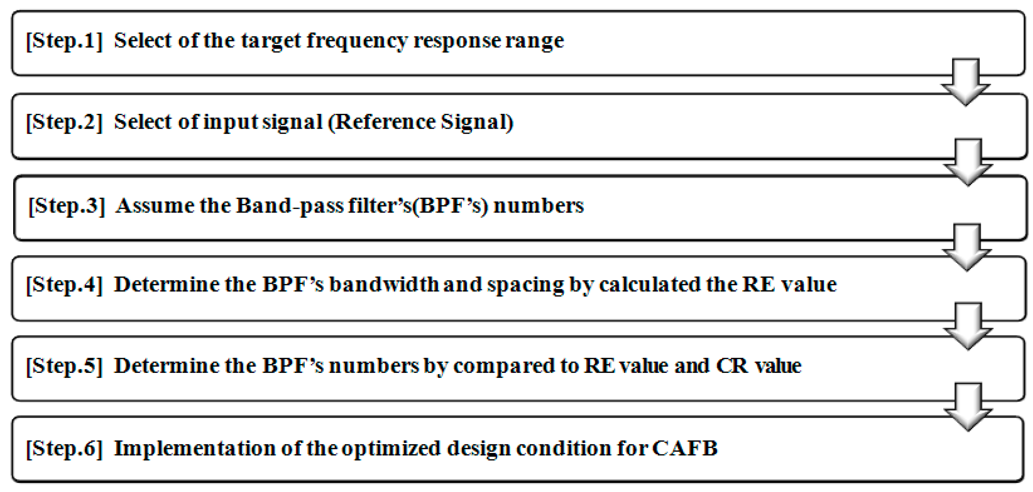Figure 4 shows the optimally-designed process of the CAFB for SHM on long and large-scale civil structures.

In Step 1, to optimize the CAFB, the interested frequency should be selected as shown in Figure 4. To do that, in the previous study, the interested frequency range of the band-pass filter is set at a frequency lower than 10 Hz. In general, the natural vibration frequency of long and large-scale civil structures is lower than 10 Hz due to the flexible behavior characteristic of the structures. As a result, a lower frequency component than 10 Hz is significant for SHM on long and large-scale civil structures.

In Step 2, to optimize the CAFB, a reference signal is necessary for frequencies lower than 10 Hz, where the reference signal is used for the optimal design of CAFB. For this purpose, in the previous study, the El-Centro seismic waveform is adapted. As shown in Figure 5, since lower frequency components than 10 Hz are predominant in the El-Centro seismic waveform, it is possible to present sub-10 Hz frequency components very well by filtering in the optimal design of the CAFB.

It is well known that the El-Centro, Kobe, and Northridge are the leading random seismic waveforms in the construction industry. They represent an unexpected circumstance which may be possible when designing, constructing, and managing structures. To assess the applicability of the IDAQ system for SHM into large structures, therefore, the El-Centro seismic waveform is chosen as an original signal for the optimization of the AFB among the random seismic waveforms mentioned above. 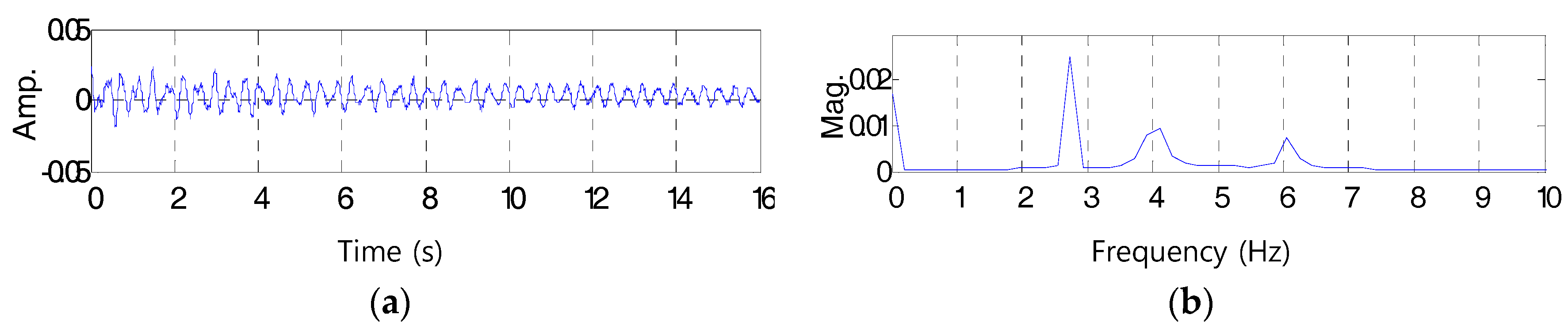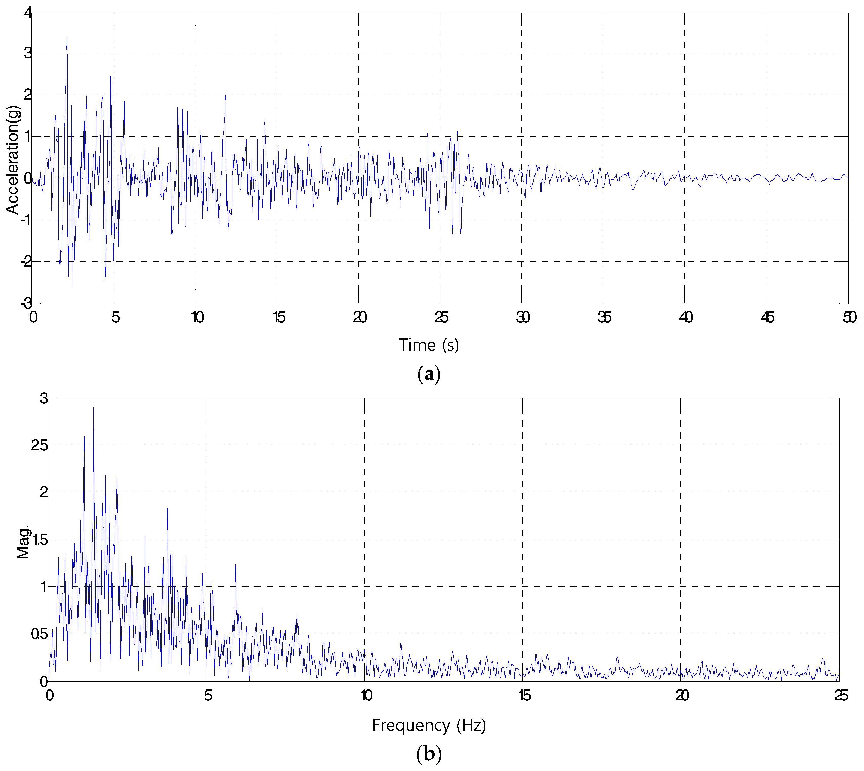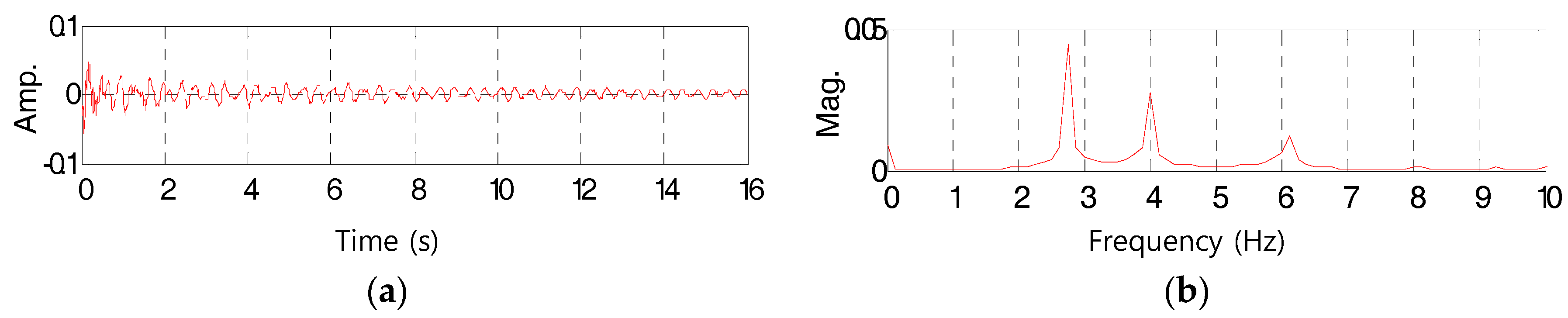Figure 5 below shows El-Centro seismic waveform (SAC name: LA02 (1940, SE)) used as an original signal, which is expressed in the time and frequency responses. According to Figure 5a, a seismic situation lasts for a short period of time (approximately one minute) in the case of El-Centro. In Figure 5b, diverse frequency factors are distributed across the frequency bands. In particular, the interested frequency is concentrated in less than 10 Hz. Here, if the seismic situation in Figure 5 is assumed, the dynamic responses of the target structure is measured as a type which includes the target structure’s own frequency factors in the conventional seismic waveform’s random frequency factors. For SHM on structures, after all, the target structure’s original frequency factors in the random frequency factors should be fully discovered. Since large structures in the construction industry usually have relatively flexible behavioral characteristics, the range of the target mode needed for SHM can be limited to a certain range of frequencies (e.g., below 10 Hz). From this perspective, the El-Centro seismic waveform selected as an original signal could be used as a reference response which can wholly express the large structure’s range of frequencies concerned (below 10 Hz). Under the assumption that an El-Centro seismic situation has these frequency characteristics, this study designs the AFB in an optimum manner based on the El-Centro seismic waveform (total time length: 50 s, delta T: 0.02 s, total frame length: 2500).

Meanwhile, when we design band-pass filters to be used in CAFB, generally, it is necessary to define three design elements for the filters, i.e., the number of filters, interval, and bandwidth. Regarding the three design elements, Peckens et al. [13,14] have established a procedure to optimize them, which contains Step 3, Step 4, and Step 5, as shown in Figure 4.

At first, in Step 3, the number of filters shall be preliminarily assumed. The number of filters can be determined by the designer’s empirical judgment considering the price and performance for the filter configuration, and the accuracy of the filtered signals. In the previous study, the number of filters is preliminarily assumed as 10. Next, in Step 4, the interval and bandwidth of the filters are decided using the number of filters assumed in Step 3. In the previous study, under the assumption that the number of filters is 10, the RE value is calculated with the condition of bandwidth for 100 intervals. The interval and bandwidth of the filter are determined corresponding to the least-calculated RE values. As the result, a 1.0 Hz interval and 0.6 Hz bandwidth are obtained. Next, in Step 5, using the interval and bandwidth derived from Step 4, the number of filters assumed in Step 3 is finally determined. In the previous study, RE and CR values are calculated under the condition of the 1.0 Hz interval and 0.6 Hz bandwidth, and 20 filters. The number of filters is determined for the position where the difference between the RE and CR value is minimized. As a result, the number of filters turned out to be six. 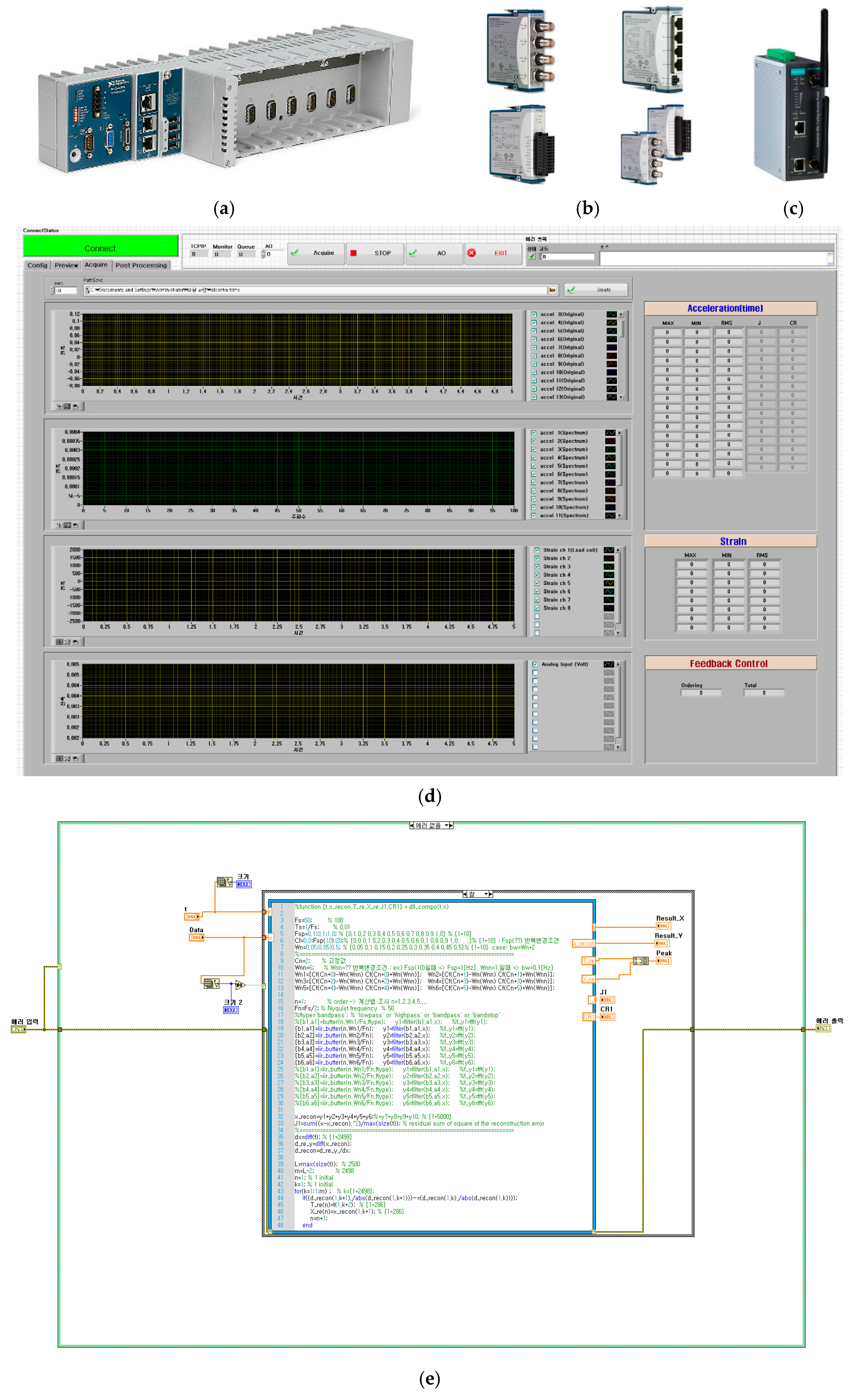Finally, in Step 6, Matlab (r2015b) from The Mathworks, Inc. (Natick, MA, USA) is utilized to program the optimal design condition (six band-pass filters, 1.0 Hz interval, and 0.6 Hz bandwidth) determined in Steps 1 to 5. Additionally, the result has been realized in a wireless measuring system using LabVIEW (2012) from National Instruments (Austin, TX, USA), which is shown in Section 3.

Furthermore, in the previous study, an analytic verification (numerical study) for the optimized CAFB is carried out so that CAFB is able to compress the dynamic response within the intended frequency range without distortion of the signal. In conclusion, the method to optimize the CAFB using the El-Centro seismic waveform can be efficient to acquire only sub-10 Hz signals from various responses of structures. If the structure to be tested has been already selected, or if it is necessary to acquire the response of a specific frequency band by filtering, the CAFB can be optimized using responses by actual measurements for the structure, or using another reference signal concentrated on a specific frequency band.

3. Data Compression Technology-Based Intelligent Data Acquisition (IDAQ) System

In this paper, a data compression technology-based IDAQ system was developed on the basis of a digital-software-design (D-S/W-D), by means of the CAFB already developed in the previous study. The CAFB is a dynamic data compression technology. It can improve on some shortcomings of wired measurement SHM, such as complicated cabling, costly installment, and constant maintenance. It also works on some restraints of wireless measurement SHM, such as limited performance of sensor nodes, analogue type of filter bank, and slow and short distance communication to make it better. The CAFB-based IDAQ system was composed of a logging & a controller system (L and Cs), a multi-I/O system (MIMO), a two-way wireless communication system (TWCs), a central monitoring and control system (CM and Cs), and embedding of the CAFB. Design and components of a CAFB-based IDAQ system are shown in Figure 6 and Figure 7.

3.1. Logging and Controller System (L and Cs)

Employing the wireless sensor nodes used in existing S-SHM systems may be difficult if the data size is increased due to an increase in the sampling ratio or expansion of the input channel, as these nodes have limitations in performance, as discussed previously. It was determined that configuring the wireless sensor nodes at the same level as a high-performance PC would be best to improve the processing speed and the storage capacity and management for the acquired data. Therefore, in this article, an Ethernet-based cDAQ-9139 provided by NI was used, as shown in Figure 6b and Figure 7a. This system is embedded with a dual-core Intel i7 processor with a clock speed of 1.33 GHz, 2 GB RAM, and 32 GB hard disk within the stand-alone chassis. This innovative system provides an improved environment in which to acquire, process, and store large datasets with high speed in real-time. Furthermore, since the L and Cs are equipped with a Linux-based RTOS, guaranteeing stability and real-time operation, it can be operated independently in real-time. Particularly, when the pre-loaded DAQ assistance and DAQmx software support are also used, diverse logics can be embedded and executed with very little manual coding. As embedded within the cDAQ-9139, the CAFB developed in Section 2 operates to compress the data, but could be utilized to replace the existing analog filter bank completely.

3.2. Multi-Input and Multi-Output System (MIMO)

For an accurate SHM of civil structures, generally quite diverse structural response analytics are required, such as for acceleration, speed, displacement, load/strain, temperature, humidity, slope, and deflection. Furthermore, for each structural response, effectively synchronized data is essential, together with stable operation in real-time. From this point of view, using independent data loggers by existing data type (static or dynamic) is no longer feasible. Therefore, in this study, a multiple input and output system (MIMO) was built, considering the multiple measurements required and the effective data synchronization required in the measuring environment to guarantee real-time operation, as shown in Figure 6d and Figure 7b. The MIMOs of the IDAQ system used the NI 9233 module, which can accommodate a piezo-type sensor group, and the NI 9237 module, which can accommodate a strain-type sensor group. Together, these two modules can acquire diverse static and dynamic data by effectively synchronizing them using the existing wire sensor group. The multiple output system of the IDAQ system used the NI 9263 module to generate an analog output signal (AO) in the range ±10 V. Furthermore, to recollect and evaluate the output signal of the NI 9263 module, the analog input-dedicated NI 9215 module was included. This MIMO configuration can be used not only for structural monitoring, but also as the integrated system for feedback control when necessary.

3.3. Two-Way Wireless Communication System (TWCs)

For bi-directional wireless communication between the cDAQ-9139, the data logging and controller system, and the host PC, the central control two-way wireless control communication system (TWCs) for the IDAQ system was the SWK-3121 module from Moxa, shown in Figure 6c and Figure 7c. This module uses industrial LAN, guaranteeing a stable wireless connection and streaming performance. The communication speed is approximately 11–54 Mbps and the basic communication distance is around 100 m. Furthermore, since it can secure up to several kilometers of additional communication distance by simply changing the RF antenna, it can be flexibly applied to the SHM systems of large civil structures.

3.4. Central Monitoring and Control System (CM&Cs)

To verify the data transmitted from the wireless sensing system regarding the condition of the civil structure, to transmit the controls according to the condition of the civil structure and to link the systems organically to prevent the data loss required for real-time control, a GUI central control system for the IDAQ system was developed using LabVIEW (2012) from National Instruments (Austin, TX, USA), running on the host PC as shown in Figure 7d.

3.5. Embedding of the CAFB

Finally, Figure 7e shows the logic for embedding the optimally-designed CAFB from the previous study. The optimally-designed CAFB in Figure 7e was programmed with software-based Matlab (r2015b) from The Mathworks, Inc. (Natick, MA, USA) code for efficient systemization. Furthermore, for the purposes of realizing and evaluating the CAFB in this paper, the test was performed by configuring the IDAQ system with the multi-input module for the acceleration channel embedded with the optimally designed CAFB and with a one-way wireless communication method activated. In addition, the operating software of the IDAQ system was comprised of data measurement, channel setup, RF communication, and multi-channel logic. The logics were programmed with LabVIEW (2012) from National Instruments (Austin, TX, USA) and utilized as the operating software of the IDAQ system.

4. Experimental Study of the CAFB Using a Model Bridge

In Section 2 and Section 3 of this paper, a CAFB was developed as the SHM of large construction structures, designed optimally using the El-Centro earthquake waveform and a wireless sensing system comprised of embedding it within the IDAQ system. In this section, the response performance of the civil structure is evaluated using the CAFB-based IDAQ system developed previously. To do that, a model bridge of the Seohae Grand Bridge in Korea, at a scale of 1/20, was designed and produced so that the targeted three low-level bending modes became less than 10 Hz to reflect the flexible dynamic characteristics of the bridge. To secure the relevance of the test value prior to the response analysis of the bridge, detailed FE (finite element) modeling and analysis were performed, and during the response test, the accuracy of the wireless response was evaluated using an IDAQ system based on the response acquired by an existing wired sensing system.

4.1. FE Analysis of Model Bridge

Prior to performing the response test of the model cable-stayed bridge using the CAFB-based IDAQ system, an eigenvalue analysis was performed through detailed FE modeling. Figure 8 and

Table 1. Design details of the model bridge.

Characteristic	Dimensions
Total/main span length	4.22 m/2.22 m
Superstructure width/Tower heights	0.17 m/1.00 m
Tower boundary conditions	Roller and hinge
Bridge end boundary conditions	Roller
Bridge material	Structural steel
Cable material	Spring (k = 1.03 N/mm)
Concentrated load	1 kg (39EA)

show the model bridge and its detailed specifications used for the FE analysis and response test.

In order to analyze the structural dynamic properties of the produced model bridge, in this paper, FE modeling-based numerical analysis was conducted. For this purpose, I-DEAS from UGS, a commercial structural analysis program, was used, and a three-dimensional detailed FE model was organized by applying the physical properties of Table 1. Here, a 1D beam element was considered for the bridge deck and the tower of the structure, the rigid element was considered for the bridge deck boundary conditions, a 1D rod element was considered for the cable; and, as for the floor beam and lumped mass, a 1 kg-size of lumped mass was considered for each of the 39 nodes, which are the positions of the floor beams on the area of the central bridge deck excluding the pylon and both sides. Next, as for the boundary condition, a clamp was considered for the substructure of the pylon, a roller was considered for both sides of the superstructure and the right-side pylon connection, and a pin was considered for the left-side pylon connection. Next, as for the degree of freedom condition of the structure, the DOF was given in the direction of y-axis with the 39 nodes on the central bridge deck as the base to complete the three-dimensional detailed FE model. Finally, considering that the sensor position can be determined later by the target mode response, an eigenvalue analysis was performed using the Guyan reduction method [28], which can analyze the modal characteristics based on the finite DOF. The detailed FE model completed for the model bridge is shown in Figure 9 and the eigenvalues for the three low-level bending modes are shown in

Table 2. Results of FE analysis of the model bridge.

	Natural Frequency & Mode Shape
1st bending mode
	2.877 Hz
2nd bending mode
	4.194 Hz
3rd bending mode
	6.242 Hz

.

4.2. Modal Test of Model Bridge

To evaluate the performance of the CAFB-based IDAQ system, the modal test was performed by using the dynamic wired measuring system. The acceleration response in the vertical direction was obtained by selecting the position (at the 1/3 point of the main span) for both the wire and wireless acceleration response using an accelerometer (Dytran model 3134D). Figure 10 shows the dynamic wire and wireless measuring systems (IDAQ system) that were utilized; the dynamic wired measuring system used the iOtech (Model: 652U) from Measurement Computing Corporation (Norton, MA, USA) and ME’ScopeVES from Vibrant Technology (Centennial, CO, USA).

Figure 11 and Figure 12 show the raw data for the (a) time and the (b) frequency domains acquired by the dynamic wire and wireless measuring systems, respectively, and

Table 3. Comparison of the natural frequency (FE analysis and wireless vs. wired signal).

Bending	Wired (Hz)	FE Analysis (Hz)	Error Ratio (%)	Wireless (Hz)	Error Ratio (%)
1st	2.735	2.877	5.191	2.736	0.036
2nd	4.005	4.194	4.719	4.104	2.471
3rd	6.154	6.242	1.429	6.058	1.559

shows the natural frequency analysis results for the raw data measured by both systems. Here, the natural frequencies for the three low-level bending modes were calculated, and the validity of the dynamic wireless sensing system configured in this article were evaluated by comparing the error ratio of the natural frequency based on the results obtained by the wired measuring system.

The FE analysis results for the natural frequency displayed errors between approximately 1.4% and 5.2% compared to the wired measurement results and, thus, the conformity was excellent. It was observed that the detailed FE model configured in Section 4.1 successfully reproduced the dynamic characteristics of the model bridge. Additionally, as the wireless measurement results showed errors of between just 0.0036% and 2.471%, compared to the wire measurement results, it was determined that the IDAQ system configured in this article is valid.

5. Evaluation of IDAQ System

5.1. Reconstruction Signal of IDAQ System

In Section 4, it was verified that the quality of the wireless response acquired by the CAFB-based IDAQ system was excellent. In this section, the performance of the CAFB-based IDAQ system is evaluated quantitatively based on the reconstruction error in Equation (1) and the compression ratio in Equation (3). The artificial filter bank embedded in the dynamic wireless measuring system was designed with a total of six band-pass filters, a filter bandwidth of 0.6 Hz, and filters at intervals of 1.0 Hz. The design conditions were optimized to acquire the structural response of the civil structure from the model bridge for a frequency range less than 10 Hz, assuming that the representative random waveform (the El-Centro earthquake) is applied to the civil structure. Since, generally, a catastrophic situation (earthquake, gust, shock, etc.), will inevitably assume a random effect on the structural response of the civil structure, this study focused on acquiring the structural response within a frequency range under 10 Hz for the structure of the model bridge to pick a target mode assuming random loading conditions in the design. Figure 13 shows the comparison results between the raw data before applying the CAFB and the reconstruction signal after applying CAFB, for both the time and frequency domain when acquiring the dynamic response by the wireless measuring system (IDAQ system).

In Figure 13, it can be observed that the reconstruction signal contained and reproduced the mode information of the raw data well enough and, as a result, it was determined that the band-pass optimizing algorithm of the artificial filter bank was effective in highlighting and expressing the target mode of interest within the frequency range of 10 Hz, achieving the goals of the initial design.

5.2. Compressive Signal of the IDAQ System

Next, for the data compression technology required to operate and manage the wireless (RF) communication and measurement database of this study, the peak-picking algorithm was designed and reflected in the artificial filter bank, and the peak signal in the time and frequency domains were picked based on the reconstruction signal and compared as shown in Figure 14. Figure 14 shows a diagraming of the reconstruction and compression signals that were created in the signal processing on the first and second stage of the CAFB, in comparison with primitive ones. They were found to faithfully reflect the modal information of primitive signals.

Additionally, in Figure 14a, only the peak values of the reconstruction signal were selected by the peak-picking algorithm completely and in Figure 14b, the mode information was clearly contained in the peak signal. Therefore, it was observed that the peak-picking algorithm was effective in selecting only the peak value containing the mode information from the entire reconstruction signal.

To evaluate the response performance of the CAFB shown in Figure 14 quantitatively, the error ratios for the frequency for the reconstruction signal and the peak signal compared to the wireless raw data are shown in

Table 4. Comparison of the natural frequency (reconstruction and compressive. vs. wireless raw signal).

Bending	Wireless (Hz)	Reconstruction (Hz)	Error Ratio (%)	Compressive (Hz)	Error Ratio (%)
1st	2.736	2.736	0.000	2.735	0.036
2nd	4.104	4.104	0.000	4.005	2.412
3rd	6.058	6.058	0.000	6.057	0.016

, and the reconstruction efficiency of the reconstruction signal compared to the raw data was calculated and shown in

Table 5. Performance of CAFB (reconstruction and compressing effectiveness).

RE	Reconstruction Efficacy (%)	CR	Compressive Efficacy (%)
0.4461	55.39	0.095	90.5

. In Table 4, the natural frequency in the reconstruction signal exactly matched that of the raw data, and the error ratio of the natural frequency in the peak signal was less than 2.5%, completely reflecting the mode information of the raw data. In Table 5, the reconstruction error and the compression ratio were 0.4461 and 0.095, respectively, meaning the developed CAFB can expect to effectively reproduce 55.39% of the signal with 90.5% of the data compression compared to the entire response signals.

6. Conclusions

In this study, an empirical study based on previous research into a cochlea-inspired artificial filter (CAFB) bank for SHM was performed. To do that, a data compression technology-based intelligent data acquisition (IDAQ) system was developed based on digital software design by embedding the previously developed CAFB into the wireless sensing system. The following conclusions were obtained by applying the developed CAFB-based IDAQ system to a model bridge and performing modal testing.

• The band-pass filter optimizing algorithm of the developed CAFB was effective in acquiring just the frequency signal containing the significant modes of interest) out of the wide frequency contents of random signals. In particular, the artificial filter bank optimized by using the representative random waveform (based on the El-Centro earthquake) can be utilized as a technology to acquire the dynamic response of large civil structures with a frequency range below 10 Hz.
• The peak-picking algorithm of the developed CAFB is effective in compressing the data size by selectively re-sampling only the peak values containing the valid modal information out of the random dynamic responses. This data compression technology can be efficiently used as a technology to operate and manage the measurement DB and also to overcome the limitations of wireless RF communications, which has emerged in WSN-based SHM technology.
• The CAFB can be optimized flexibly with a random standard signal, and it can be utilized as a technology to acquire the dynamic response not only from civil structures, but also from other structures (e.g., machines used in industry). Furthermore, it was observed that the reconstruction signal and compressive signal evaluated in this study are not only capable of reconstructing in the time domain but also reflect the modal information of the frequency domain.
• In this paper, CAFB was optimized on the basis of three target modes in order to efficiently acquire dynamic responses concerned on the model structure, and its performance was quantitatively evaluated through modal experiments. If the target structure is not a civil structure, but a machine, a plant, or other facilities whose frequency of dynamic responses is different from the one concerned in this paper, it can be newly optimized for a new purpose. The CAFB, which was evaluated in this paper can, thus, be variably applied with flexible readjustment and optimization in regard to the range of frequency and responses of a target structure.
• Ultimately, since the CAFB-based IDAQ system developed in this study can acquire the compressed size of the valid dynamic response around the frequency range of interest it is, therefore, relevant with respect to the economy and efficiency when measuring the dynamic response of civil structures in real-time and it is determined that this system can provide a new paradigm for structural health monitoring using WSNs.
• Additionally, since this research is based on indoor experiments based on a model structure, it should be pointed out that further studies are needed to find the effect of environmental conditions and season variability in the wireless reading, etc.