Surface Waves Propagating on Grounded Anisotropic Dielectric Slab

Abstract

This paper investigates the characteristics of surface waves propagating on a grounded anisotropic dielectric slab. Distinct from the existing analyses that generally assume that the fields of surface wave uniformly distribute along the transverse direction of the infinitely large grounded slab, our method takes into account the field variations along the transverse direction of a finite-width slab. By solving Maxwell’s equations in closed-form, it is revealed that no pure transverse magnetic (TM) or transverse electric (TE) mode exists if the fields are non-uniformly distributed along the transverse direction of the grounded slab. Instead, two hybrid modes, namely quasi-TM and quasi-TE modes, are supported. In addition, the propagation characteristics of two hybrid modes supported by the grounded anisotropic slab are analyzed in terms of the slab thickness, slab width, as well as the relative permittivity tensor of the anisotropic slab. Furthermore, different methods are employed to compare the analyses, as well as to validate our derivations. The proposed method is very suitable for practical engineering applications.

1. Introduction

Over recent decades, surface waves have attracted extensive attention due to their unique characteristics of existing at the interface of two different media with the field exponentially decaying away from the interface. For example, Dyakonov surface waves have been investigated thoroughly in several literatures [1,2,3]. The characteristics of the surface waves propagating at the interfaces between isotropic-to-isotropic, isotropic-to-anisotropic, and isotropic-to-indefinite media have been rigorously studied in [4,5,6,7,8]. Moreover, surface waves have also been found in many structures, such as dielectric rod [9], uniaxial and biaxial slab waveguides [10,11], plasma slab [12], chiral material [13], and photonic crystal [14], to name only a few.

Among all of the geometries of supporting surface waves, one of the best-known structures is the grounded dielectric slab. It is known that the infinitely large grounded dielectric slab can support pure transverse magnetic (TM) and transverse electric (TE) surface wave modes, and their propagating constants on isotropic slab were analyzed in [4], the corresponding fields and power of the surface waves were studied in [15]. In addition to the case of isotropic grounded slab, the guidance conditions of TM and TE surface waves in grounded anisotropic slab were considered in [16]. The solution of suppressing surface waves on grounded anisotropic slab was explored in [17]. Furthermore, investigations were also focused on the radiation conditions of surface wave on grounded dielectric slabs, which have been employed for designing wideband, low-profile, as well as high gain antennas [18,19,20].

Although a lot of studies have been carried out to characterize surface waves propagating along a grounded dielectric slab, the analyses only focus on structures that are of infinite length and width, and assume that there is no field variation along the direction orthogonal to the propagation direction of surface waves. To the best of our knowledge, no detailed analysis has been introduced for the case that the fields are non-uniformly distributed along the direction transverse to the propagation direction, which is a more practical concern for most engineers. In addition, most substrates used in real applications exhibit nonnegligible anisotropic properties due to either the intrinsic anisotropy of the material or the manufacturing process [21]. The effect of the anisotropy of the material on the propagation characteristics of surface waves is another concern for practical engineering.

This paper investigates the characteristics of surface waves propagating on a grounded anisotropic dielectric slab, especially focuses on the slab with finite width. By assuming that the surface waves are propagating along the longitudinal direction of the slab, the field variations along the transverse direction are considered. Different methods are compared to analyze the propagation characteristics, as well as to validate our derivations. The main contributions of our work are as follows. (i) It is revealed that no pure TM or TE mode exists on the grounded infinitely large slab if the field is non-uniformly distributed along the direction orthogonal to the propagation direction; (ii) Closed-form analytical expressions are derived to theoretically study the characteristics of quasi-TM and quasi-TE surface modes on the finite-width grounded anisotropic grounded slab. It is found that surface waves propagate away from the longitudinal direction of the finite-width slab with some certain angle, and the angle decreases as the slab width increases; (iii) Different from the existing analyses of surface waves whose fields distribute uniformly along the transverse direction of the infinitely large slab, our method takes into account the variations of the fields distributed on the transverse direction of the grounded anisotropic slab, which has a more practical relevance and can provide a more accurate solution for engineering applications such as designing wideband and high gain antennas based on grounded dielectric slabs [9,18,19,20]. It is worth mentioning that our method is also suitable for grounded isotropic dielectric slab.

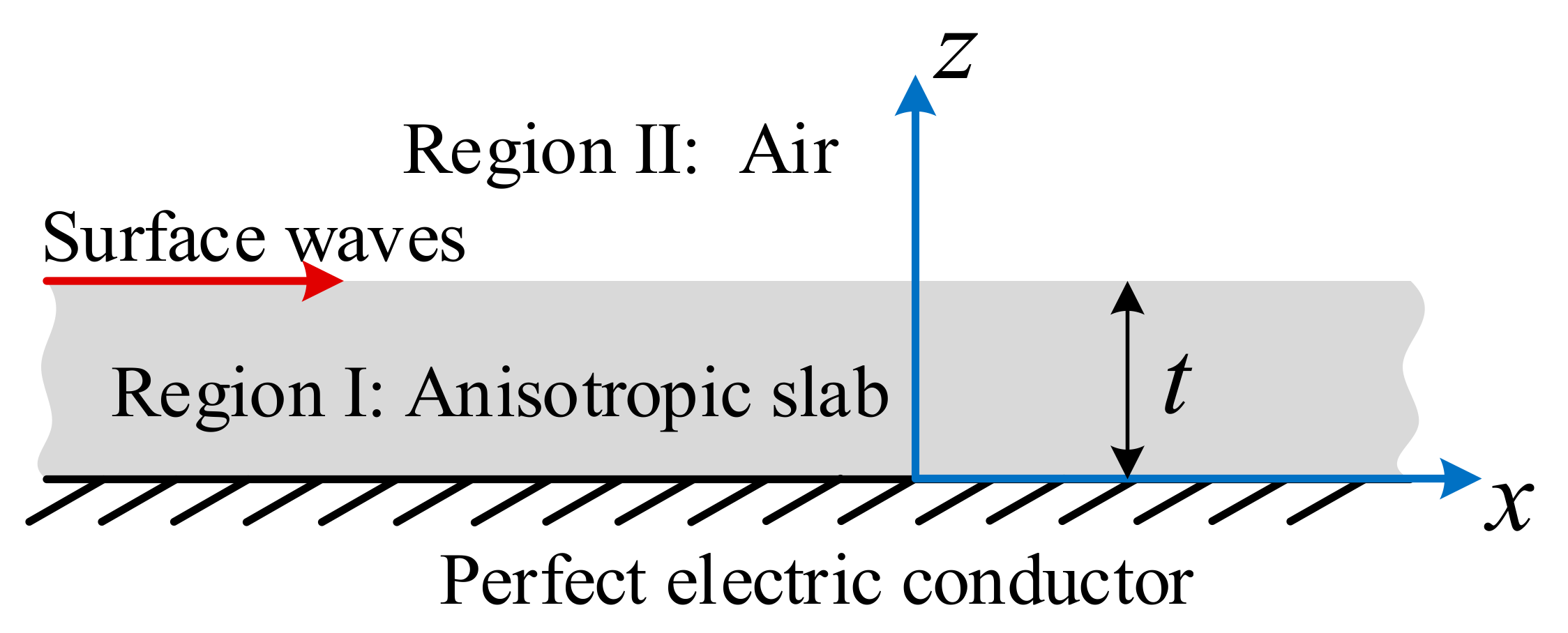
2. Characteristics of Surface Waves Propagating on Grounded Anisotropic Slab

2.1. Infinitely Large Anisotropic Grounded Slab

Figure 1 shows the geometry of the anisotropic slab backed by a perfect electric conductor. We assume that the grounded slab is infinite in both x and y directions, the surface waves propagate along the longitudinal +x direction with an $e^{-j{\beta }_{x}x}$ propagation factor. The thickness of the slab is t. The slab is considered as anisotropic as a general discussion, and the relative permittivity $\stackrel{=}{\mathit{\epsilon }}$ and permeability $\stackrel{=}{\mathit{\mu }}$ of the anisotropic slab are expressed as:

$$\stackrel{=}{\mathit{\epsilon }}=\left[\begin{array}{ccc}{\epsilon }_x& 0& 0\\ 0& {\epsilon }_y& 0\\ 0& 0& {\epsilon }_z\end{array}\right], \stackrel{=}{\mathit{\mu }}=\left[\begin{array}{ccc}{\mu }_x& 0& 0\\ 0& {\mu }_y& 0\\ 0& 0& {\mu }_z\end{array}\right],$$

(1)

where the diagonal elements represent the eigenvalues of $\stackrel{=}{\mathit{\epsilon }}$ and $\stackrel{=}{\mathit{\mu }}$, respectively, and their directions constitute the principle axes of the anisotropic slab. In order to analyze the characteristics of surface waves propagating along the grounded anisotropic dielectric slab, we separately consider the fields in anisotropic and air regions, then solve Maxwell’s equations and apply boundary conditions across the interface. For the considered structure, the E-field and H-field along the x direction for both regions are expressed as:

Region I

$$E_x^{\mathrm{I}}=A_{\mathrm{I}}{f}_e\left(y\right)e^{-j{\beta }_{x}x}\sin \left(k_{z}z\right),$$

(2)

$$H_x^{\mathrm{I}}=B_{\mathrm{I}}{f}_h\left(y\right)e^{-j{\beta }_{x}x}\cos \left(k_{z}z\right),$$

(3)

Region II

$$E_x^{\mathrm{II}}=A_{\mathrm{II}}{f}_e\left(y\right)e^{-j{\beta }_{x}x}{\mathrm{e}}^{-k_{0z}z},$$

(4)

$$H_x^{\mathrm{II}}=B_{\mathrm{II}}{f}_h\left(y\right)e^{-j{\beta }_{x}x}{\mathrm{e}}^{-k_{0z}z},$$

(5)

where A_I, A_II, B_I, and B_II are the amplitude coefficients of the corresponding fields in each region. β_x is the phase constant of surface waves along the x direction. k_z is the wavenumber in the anisotropic medium in the z direction. The sine function of $E_x^{\mathrm{I}}$ and cosine function of $H_x^{\mathrm{I}}$ in the anisotropic medium are selected due to the vanishing electric field and maximum magnetic field on the perfect electric conductor (PEC) ground plane, respectively. Due to the fields of surface waves decaying exponentially away in air from the interface, the z component of fields in air region is expressed as ${\mathrm{e}}^{-k_{0z}z}$, with k₀z real and positive. In addition, f_e(y) and f_h(y) represent the y components of E-field and H-field, respectively. For the infinitely large slab, we assume that the propagation constant in the y direction is R_y, f_e(y) and f_h(y), then satisfy the following form:

$$f_e\left(y\right)=f_h\left(y\right)=f\left(y\right) =\{\begin{array}{c}{e}^{-R_{y}y} \left(y\ge 0\right)\\ e^{R_{y}y} \left(y\le 0\right)\end{array}.$$

(6)

If R_y = 0, then ∂f(y)/∂y = 0, which indicates that the field has no variation in the y direction. On the other hand, if R_y ≠ 0, the field of surface wave is non-uniformly distributed along the y direction.

By solving Maxwell’s equations based on Equations (2)–(5), the E- and H-fields in both anisotropic slab and air regions in y and z directions are found as:

Region I

$$E_y^{\mathrm{I}}=\frac{e^{-j{\beta }_{x}x}\sin \left(k_z\mathrm{z}\right)}{j\left({\epsilon }_y{\mu }_z{k}_0^2-{\beta }_x^2\right)}[{\beta }_x{A}_{\mathrm{I}}\frac{\partial f_e\left(y\right)}{\partial y}-\omega {\mu }_0{\mu }_z{k}_z{B}_{\mathrm{I}}{f}_h\left(y\right)],$$

(7)

$$H_y^{\mathrm{I}}=\frac{e^{-j{\beta }_{x}x}\cos \left(k_z\mathrm{z}\right)}{j({\epsilon }_z{\mu }_y{k}_0^2-{\beta }_x^2)}[{\beta }_x{B}_{\mathrm{I}}\frac{\partial f_h\left(y\right)}{\partial y}-\omega {\epsilon }_0{\epsilon }_z{k}_z{A}_{\mathrm{I}}{f}_e\left(y\right)],$$

(8)

$$E_z^{\mathrm{I}}=\frac{e^{-j{\beta }_{x}x}\cos \left(k_z\mathrm{z}\right)}{j\left({\epsilon }_z{\mu }_y{k}_0^2-{\beta }_x^2\right)}[{\beta }_x{k}_z{A}_{\mathrm{I}}{f}_e\left(y\right)-\omega {\mu }_0{\mu }_y{B}_{\mathrm{I}}\frac{\partial f_h\left(y\right)}{\partial y}],$$

(9)

$$H_z^{\mathrm{I}}=\frac{e^{-j{\beta }_{x}x}\sin \left(k_z\mathrm{z}\right)}{j\left({\epsilon }_y{\mu }_z{k}_0^2-{\beta }_x^2\right)}[-{\beta }_x{k}_z{B}_{\mathrm{I}}{f}_h\left(y\right)+\omega {\epsilon }_0{\epsilon }_y{A}_{\mathrm{I}}\frac{\partial f_e\left(y\right)}{\partial y}].$$

(10)

Region II

$$E_y^{\mathrm{II}}=\frac{e^{-j{\beta }_{x}x} e^{-k_{0z}z}}{j\left(k_0^2-{\beta }_x^2\right)}[{\beta }_x{A}_{\mathrm{II}}\frac{\partial f_e\left(y\right)}{\partial y}-\omega {\mu }_0{k}_{0z}{B}_{\mathrm{II}}{f}_h\left(y\right)],$$

(11)

$$H_y^{\mathrm{II}}=\frac{e^{-j{\beta }_{x}x} e^{-k_{0z}z}}{j\left(k_0^2-{\beta }_x^2\right)}[{\beta }_x{B}_{\mathrm{II}}\frac{\partial f_h\left(y\right)}{\partial y}+\omega {\epsilon }_0{k}_{0z}{A}_{\mathrm{II}}{f}_e\left(y\right)],$$

(12)

$$E_z^{\mathrm{II}}=\frac{e^{-j{\beta }_{x}x} e^{-k_{0z}z}}{j\left(k_0^2-{\beta }_x^2\right)}[-{\beta }_x{k}_{0z}{A}_{\mathrm{II}}{f}_e\left(y\right)-\omega {\mu }_0{B}_{\mathrm{II}}\frac{\partial f_h\left(y\right)}{\partial y}],$$

(13)

$$H_z^{\mathrm{II}}=\frac{e^{-j{\beta }_{x}x} e^{-k_{0z}z}}{j\left(k_0^2-{\beta }_x^2\right)}[-{\beta }_x{k}_{0z}{B}_{\mathrm{II}}{f}_h\left(y\right)+\omega {\epsilon }_0{A}_{\mathrm{II}}\frac{\partial f_e\left(y\right)}{\partial y}].$$

(14)

Based on the field distributions and boundary conditions, the characteristics of the surface waves can be analyzed, as follows.

2.1.1. TM Mode Surface Wave

For the pure TM surface wave, it is known that B_I = B_II = 0, the continuity conditions of E_x and E_y at the interface z = t give

$$A_{\mathrm{I}}\sin \left(k_{z}t\right)=A_{\mathrm{II}}{e}^{-k_{0z}t},$$

(15)

$$\frac{\partial f\left(y\right)}{\partial y}\frac{A_{\mathrm{I}}\sin \left(k_{z}t\right)}{{\epsilon }_y{\mu }_z{k}_0^2-{\beta }_x^2}=\frac{\partial f\left(y\right)}{\partial y}\frac{A_{\mathrm{II}}{e}^{-k_{0z}t}}{k_0^2-{\beta }_x^2} ,$$

(16)

which lead to

$${\epsilon }_y{\mu }_z=1,$$

(17)

or

$$\frac{\partial f\left(y\right)}{\partial y}=0.$$

(18)

It is obvious that Equation (17) is not satisfied since the dielectric slab cannot be air for our discussion. Therefore, Equation (18) is the only solution, indicating that for pure TM surface wave propagating along the x direction of the grounded anisotropic slab, the field distribution along the y direction must be uniform.

2.1.2. TE Mode Surface Wave

For the pure TE surface wave, it is obvious that A_I = A_II = 0. Similarly, according to the boundary conditions of H_x and H_y at the interface z = t, Equation (18) is also satisfied.

2.1.3. Hybrid Mode Surface Wave

Based on the above discussions, it is concluded that if the pure TM or TE surface wave exists on the grounded dielectric slab, the field distribution along the y direction must be uniform. In other words, if ∂f(y)/∂y ≠ 0 or Ry ≠ 0, hybrid mode surface waves that consist of quasi-TM mode with small H_x and quasi-TE mode with small E_x propagate along the slab. In this case, the continuity of tangential fields across the interface z = t leads to:

$${\beta }_x^2{R}_y^2{k}_0^2\left(1-{\epsilon }_z{\mu }_y\right)\left(1-{\epsilon }_y{\mu }_z\right)=\left[{\epsilon }_z{k}_z\left(k_0^2-{\beta }_x^2\right)+k_{0z}\left({\epsilon }_z{\mu }_y{k}_0^2-{\beta }_x^2\right)\tan \left(k_{z}t\right)\right]\left[{\mu }_z{k}_z\left(k_0^2-{\beta }_x^2\right)-k_{0z}\left({\epsilon }_y{\mu }_z{k}_0^2 –{\beta }_x^2\right)\cot \left(k_{z}t\right)\right].$$

(19)

By applying Maxwell’s equation, the dispersion relations in both regions are:

Region I

$${\beta }_x^2{R}_y^2{k}_z^2{(\frac{1}{{\epsilon }_z{\mu }_y{k}_0^2-{\beta }_x^2}-\frac{1}{{\epsilon }_y{\mu }_z{k}_0^2-{\beta }_x^2})}^2=-k_0^2({\epsilon }_x+\frac{{\epsilon }_y{R}_y^2}{{\epsilon }_y{\mu }_z{k}_0^2-{\beta }_x^2}-\frac{{\epsilon }_z{k}_z^2}{{\epsilon }_z{\mu }_y{k}_0^2-{\beta }_x^2})({\mu }_x+\frac{{\mu }_y{R}_y^2}{{\epsilon }_z{\mu }_y{k}_0^2-{\beta }_x^2}-\frac{{\mu }_z{k}_z^2}{{\epsilon }_y{\mu }_z{k}_0^2-{\beta }_x^2}).$$

(20)

Region II

$${\beta }_x^2-R_y^2-k_{0z}^2=k_0^2.$$

(21)

From Equations (19)–(21), it is seen that three equations with four unknowns β_x, R_y, k_z, and k_oz are obtained, which implies that there is no unique solution for β_x, unless R_y is determined. It is worth mentioning that for pure TM and TE surface waves, β_x, k_z, and k_oz can be solved for given k₀, slab thickness t, and relative permittivity $\stackrel{=}{\epsilon }$ and permeability $\stackrel{=}{\mu }$ by substituting R_y = 0 into Equations (19)–(21). The above analyses can also be applied to the grounded isotropic slab, in which case we can use the relative permittivity ε_r = ε_x = ε_y = ε_z and permeability μ_r = μ_x = μ_y = μ_z, instead of $\stackrel{=}{\epsilon }$ and $\stackrel{=}{\mu }$.

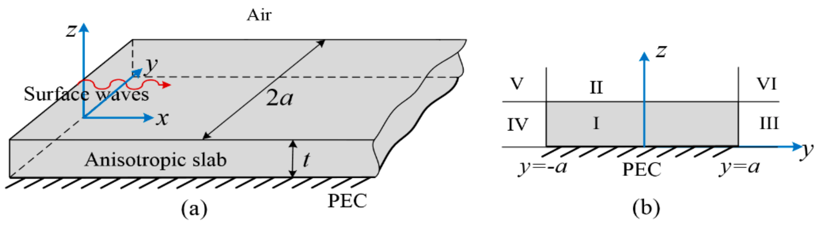
2.2. Finite-Width Anisotropic Grounded Slab

Figure 2 shows the grounded anisotropic slab with a finite width 2a and thickness t. By applying the boundary conditions at the interfaces y = ±a, the propagation constant in the y direction R_y can then be determined. For analysis, the cross-section of the grounded slab is sub-divided into six regions, as shown in Figure 2b. Region I is the anisotropic slab, while the others are air regions. Since the fields in two corner Regions V and VI are very small, which are assumed to be negligible [22], we only take into account Regions I, II, III, and IV for analysis.

The E-field and H-field along the x direction for Regions I and II have the same expressions as Equations (2)–(5). However, due to the discontinuity at y = ±a, reflected waves exist along the y direction. Therefore, the y components f_e(y) and f_h(y) of the E-Field and H-field are expressed as:

$$f_e\left(y\right)=e^{-R_{y}y}+r_1{e}^{R_{y}y},$$

(22)

$$f_h\left(y\right)=e^{-R_{y}y}+r_2{e}^{R_{y}y},$$

(23)

where r₁ and r₂ represent the magnitude ratios of $e^{R_{y}y}$ and $e^{-R_{y}y}$ for f_e(y) and f_h(y), respectively. The fields in both Regions I and II in y and z directions can be obtained by substituting Equations (22) and (23) into Equations (7)–(14).

In Regions III and IV, the fields are decaying away from the interfaces y = ±a along the y direction. Therefore, the y components of fields can be expressed as ${\mathrm{e}}^{-R_{0y}y}$ and ${\mathrm{e}}^{R_{0y}y}$, respectively. Based on the continuity conditions of the tangent fields at the interface, the E-field and H-field along the x direction for Regions III and IV are given as follows:

Region III

$$E_x^{\mathrm{III}}=A_{\mathrm{III}}{\mathrm{e}}^{-R_{0y}y}{e}^{-j{\beta }_{x}x}\sin \left(k_{z}z\right),$$

(24)

$$H_x^{\mathrm{III}}=B_{\mathrm{III}}{\mathrm{e}}^{-R_{0y}y}{e}^{-j{\beta }_{x}x}\cos \left(k_{z}z\right),$$

(25)

Region IV

$$E_x^{\mathrm{IV}}=A_{\mathrm{IV}}{\mathrm{e}}^{R_{0y}y}{e}^{-j{\beta }_{x}x}\sin \left(k_{z}z\right),$$

(26)

$$H_x^{\mathrm{IV}}=B_{\mathrm{IV}}{\mathrm{e}}^{R_{0y}y}{e}^{-j{\beta }_{x}x}\cos \left(k_{z}z\right),$$

(27)

where A_III, B_III, A_IV, and B_IV are corresponding amplitude coefficients. The E-field and H-field in the y and z directions can then be found as:

Region III

$$E_y^{\mathrm{III}}=\frac{e^{-j{\beta }_{x}x}{\mathrm{e}}^{-R_{0y}y}\sin \left(k_z\mathrm{z}\right)}{j\left(k_0^2-{\beta }_x^2\right)}\left[-{\beta }_x{R}_{0y}{A}_{\mathrm{III}}-\omega {\mu }_0{k}_z{B}_{\mathrm{III}}\right],$$

(28)

$$H_y^{\mathrm{III}}=\frac{e^{-j{\beta }_{x}x}{\mathrm{e}}^{-R_{0y}y}\cos \left(k_z\mathrm{z}\right)}{j\left(k_0^2-{\beta }_x^2\right)}\left[-{\beta }_x{R}_{0y}{B}_{\mathrm{III}}-\omega {\epsilon }_0{k}_z{A}_{\mathrm{III}}\right],$$

(29)

$$E_z^{\mathrm{III}}=\frac{e^{-j{\beta }_{x}x}{\mathrm{e}}^{-R_{0y}y}\cos \left(k_z\mathrm{z}\right)}{j\left(k_0^2-{\beta }_x^2\right)}[{\beta }_x{k}_z{A}_{\mathrm{III}}+\omega {\mu }_0{R}_{0y}{B}_{\mathrm{III}}],$$

(30)

$$H_z^{\mathrm{III}}=\frac{e^{-j{\beta }_{x}x}{\mathrm{e}}^{-R_{0y}y}\sin \left(k_z\mathrm{z}\right)}{j\left(k_0^2-{\beta }_x^2\right)}\left[-{\beta }_x{k}_z{B}_{\mathrm{III}}-\omega {\epsilon }_0{R}_{0y}{A}_{\mathrm{III}}\right].$$

(31)

Region IV

$$E_y^{\mathrm{IV}}=\frac{e^{-j{\beta }_{x}x}{\mathrm{e}}^{R_{0y}y}\sin \left(k_z\mathrm{z}\right)}{j\left(k_0^2-{\beta }_x^2\right)}\left[{\beta }_x{R}_{0y}{A}_{\mathrm{IV}}-\omega {\mu }_0{k}_z{B}_{\mathrm{IV}}\right],$$

(32)

$$H_y^{\mathrm{IV}}=\frac{e^{-j{\beta }_{x}x}{\mathrm{e}}^{R_{0y}y}\cos \left(k_z\mathrm{z}\right)}{j\left(k_0^2-{\beta }_x^2\right)}\left[{\beta }_x{R}_{0y}{B}_{\mathrm{IV}}-\omega {\epsilon }_0{k}_z{A}_{\mathrm{IV}}\right],$$

(33)

$$E_z^{\mathrm{IV}}=\frac{e^{-j{\beta }_{x}x}{\mathrm{e}}^{R_{0y}y}\cos \left(k_z\mathrm{z}\right)}{j\left(k_0^2-{\beta }_x^2\right)}[{\beta }_x{k}_z{A}_{\mathrm{IV}}-\omega {\mu }_0{R}_{0y}{B}_{\mathrm{IV}}],$$

(34)

$$H_z^{\mathrm{IV}}=\frac{e^{-j{\beta }_{x}x}{\mathrm{e}}^{R_{0y}y}\sin \left(k_z\mathrm{z}\right)}{j\left(k_0^2-{\beta }_x^2\right)}\left[-{\beta }_x{k}_z{B}_{\mathrm{IV}}+\omega {\epsilon }_0{R}_{0y}{A}_{\mathrm{IV}}\right].$$

(35)

The boundary condition across the interface z = t provides the same result as Equation (19), while the field continuities at the interfaces y = ±a give

$${\beta }_x^2{k}_z^2\left(\frac{1}{{\epsilon }_z{\mu }_y{k}_0^2-{\beta }_x^2}-\frac{1}{k_0^2-{\beta }_x^2}\right)\left(\frac{1}{{\epsilon }_y{\mu }_z{k}_0^2-{\beta }_x^2}-\frac{1}{k_0^2-{\beta }_x^2}\right)=k_0^2\left(-\frac{{\mu }_y{R}_y}{{\epsilon }_z{\mu }_y{k}_0^2-{\beta }_x^2}+\frac{R_{0y}}{k_0^2-{\beta }_x^2}\frac{e^{-R_{y}a}-r_1{e}^{R_{y}a}}{e^{-R_{y}a}+r_1{e}^{R_{y}a}}\right)\left(-\frac{{\epsilon }_y{R}_y}{{\epsilon }_y{\mu }_z{k}_0^2-{\beta }_x^2}+\frac{R_{0y}}{k_0^2-{\beta }_x^2}\frac{e^{-R_{y}a}+r_1{e}^{R_{y}a}}{e^{-R_{y}a}-r_1{e}^{R_{y}a}}\right),$$

(36)

and

$$r_1=-r_2=\{\begin{array}{c}1 quasi-TM mode\\ -1 quasi-TE mode\end{array}$$

(37)

In addition, the dispersion relation of both Regions III and IV can be found as

$${\beta }_x^2-R_{0y}^2+k_z^2= k_0^2.$$

(38)

Therefore, from Equations (19)–(21) and (36)–(38), it is seen that six equations with six unknowns β_x, R_y, R_oy, k_z, k_oz, and r₁ are derived, so that the propagation characteristics of the quasi-TM and quasi-TE surface waves can be determined.

3. Numerical Analysis

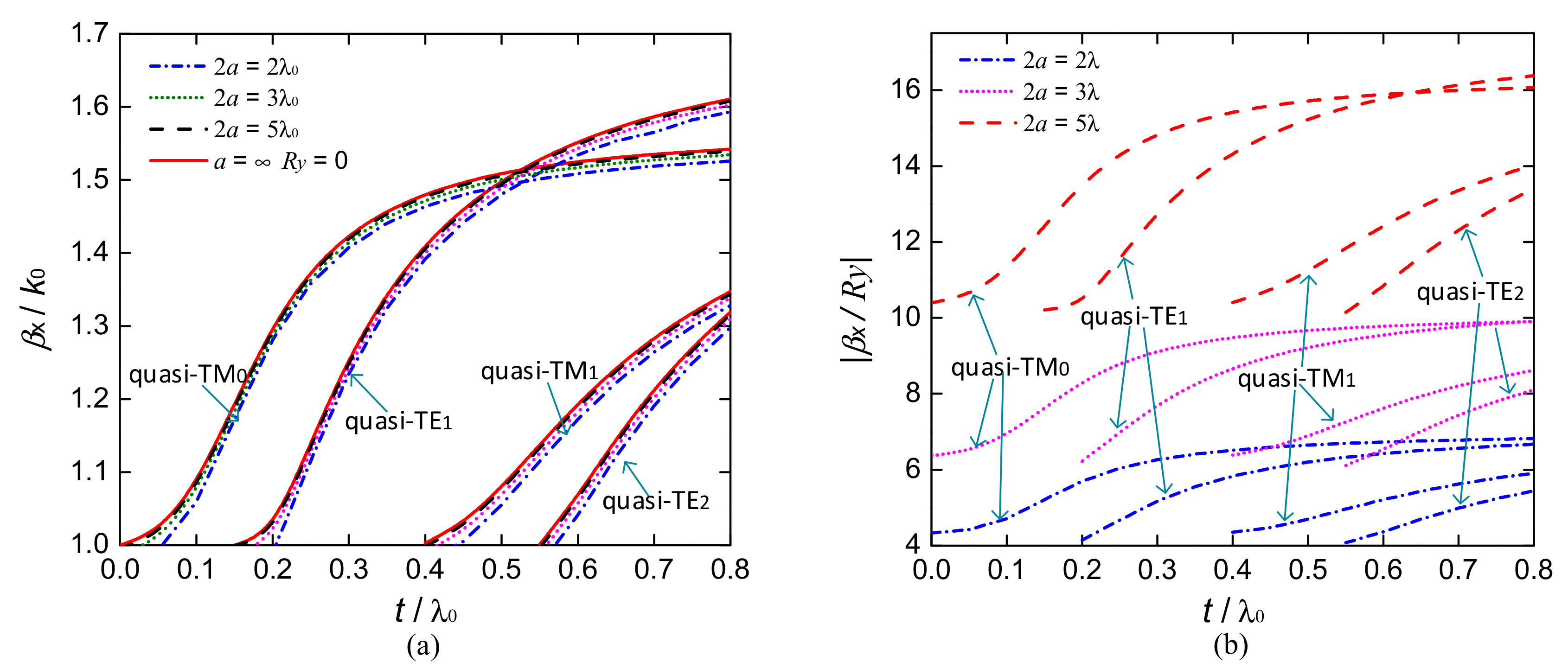
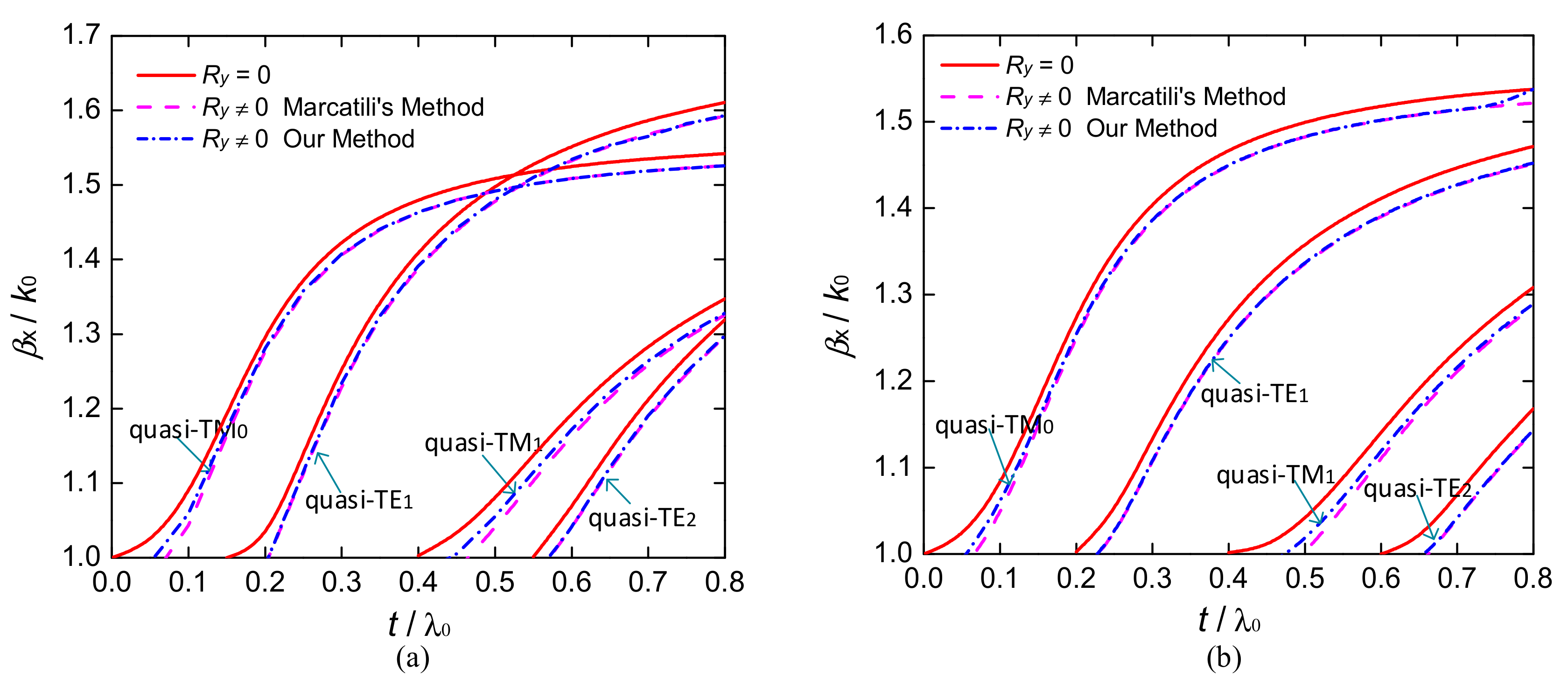
3.1. Comparion of Different Methods

In this section, three different methods are employed to compare the propagation characteristics of surface waves on an anisotropic grounded dielectric slab. In the first method, it is assumed that the slab is infinitely large in both x and y directions, and there is no field variation along the y direction. This method has been utilized in most open literature, but it can only provide approximate results for real engineering applications, in which finite-width slabs are usually employed, and the field distributions along the y direction are non-uniform. The propagation characteristics are summarized in Equations (A1)–(A6) in Appendix A. The second method is based on Marcatili’s method [22]. This method considers the field variations along the y direction of the finite-width slab. However, the analysis assumes that H_z = 0 and H_y = 0 for quasi-TM and quasi-TE modes, respectively. Based on this approximate method, we derived the closed-form expressions for propagation characteristics of quasi-TM and quasi-TE modes for the considered structure, which can be obtained using Equations (A8)–(A12) and (A14)–(A18), respectively, as summarized in Appendix B. The third one is based on our derivations by using Equations (19)–(21) and (36)–(38). In our method, hybrid surface wave modes on grounded dielectric slab with finite width are analyzed, which addresses the main concern and provides a more accurate solution for practical applications.

As an example, we use an anisotropic PTFE substrate in [21] with ε_x = 2.95, ε_y = 2.89, ε_z = 2.45, and μ_x = μ_y = μ_z = 1 to analyze the propagation constants of surface waves, and the results at f = 16 GHz are shown in Figure 3a. In addition, the corresponding results of isotropic slab with ε_x = ε_y = ε_z = 2.45 and μ_x = μ_y = μ_z = 1 are also shown in Figure 3b for comparison. In our calculation, we are looking for solutions that surface waves propagate along the x direction and decay in the z direction away from the interface, so that β_x and k_0z should be positive real numbers. For the first method, the slab width is assumed to be infinite with R_y = 0, while for the other two methods, the slab width is set as 2a = 37.5 mm, with R_y ≠ 0. Figure 3a,b both indicate that the results of finite-width slab obtained by Macatili’s method and our method are very close. However, it is interesting to note that for a fixed slab thickness, the propagation constant β_x obtained from the finite-width slab (R_y ≠ 0) is smaller than that from the infinite one (R_y = 0). In other words, in order to excite the same order of surface waves with an equal β_k, the finite-width slab should be thicker than the infinite one. In addition, it is seen that as the thicknesses of finite- and infinite-width slabs decease, the finite one can reach the condition β_k/k₀ = 1 with a larger t. Under this condition, the surface waves will transform into leaky waves. Furthermore, comparing the case of anisotropic with isotropic slabs, it is seen that the anisotropic property of the slab has significant effects on both quasi-TM and quasi-TE modes, which will be discussed in detail in the next section.

As shown in Figure 4a, the values of β_x/k₀ as a function of t/λ₀ with different slab widths are compared. In this study, our method based on Equations (19)–(21) and (36)–(38) is employed for the case of finite-width slab, while for the case of a = ∞, the first method is utilized. It is seen that when the slab width increases, the values of β_x/k₀ increase, and they are closer to the case of a = ∞ with R_y = 0. This phenomenon also validates our derivations in a way. Furthermore, it is worth pointing out that the propagation constant in the y direction R_y is revealed to be a pure imaginary number in our calculation, which indicates that the surface waves propagate along the y direction in addition to the x direction, so that the propagating direction deviates from the x direction with some certain angle. The values of |β_x/R_y| as a function of t/λ₀ with different slab widths are plotted in Figure 4b. The results indicate that |β_x/R_y| is very sensitive to the slab width. When the slab width increases, then the value of |β_x/R_y| increases significantly, meaning that the propagation direction is closer to the x direction.

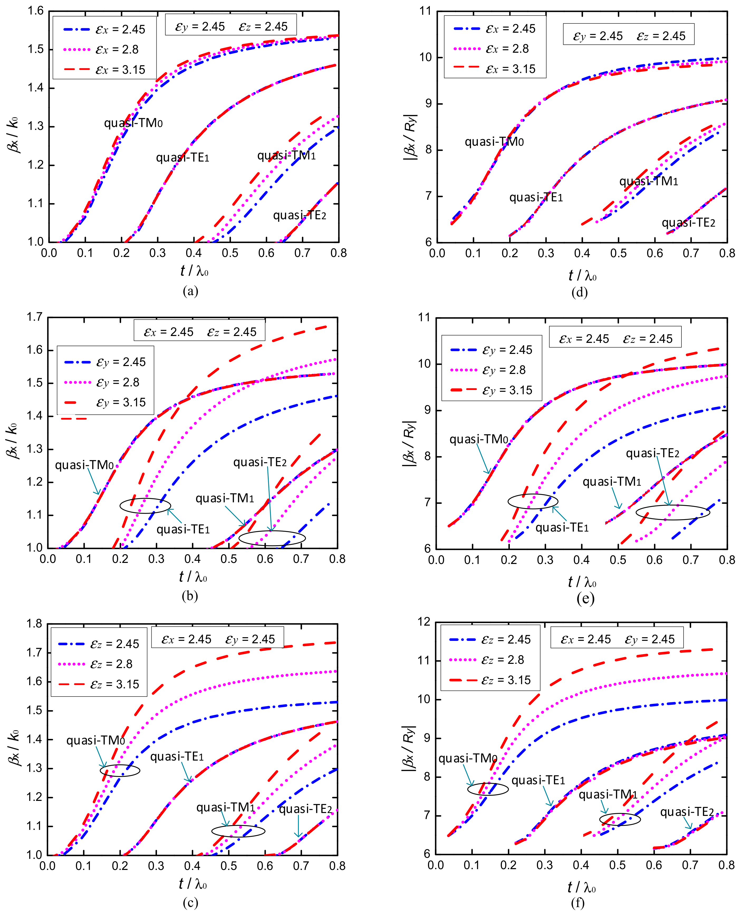
3.2. Effects of Permittivity Tensor on Propagation Characteristics of Surface Waves

The effects of the relative permittivity tensor on propagation characteristics of surface waves are investigated. Based on Equations (19)–(21) and (36)–(38), the corresponding values of β_x/k₀ and |β_x/R_y| as a function of slab thickness are calculated. As an instance, the calculated frequency is set as f = 16 GHz, and the slab width is 2a = 56.25 mm.

Figure 5a,d show the effects of ε_x on β_x/k₀ and |β_x/R_y| as a function of slab thickness. It is seen that when both ε_y and ε_z remain to be 2.45 and the value of ε_x varies from 2.45 to 3.15, β_x/k₀, and |β_x/R_y| are almost stable for quasi-TE modes. However, the corresponding values of quasi-TM modes slightly change with the increase of ε_x. Similarly, the effects of ε_y and ε_z on the propagation characteristics of surface waves are also investigated. Figure 5b,e illustrate that slightly increasing ε_y results in a significant increase of β_x/k₀ and |β_x/R_y| for quasi-TE modes, while the quasi-TM modes are nearly unaffected. In contrast, as shown in Figure 5c,f, the value of ε_z can significantly affect the propagation characteristics of quasi-TM modes, but hardly contributes to the quasi-TE modes. Since most of the substrates exhibit a nonnegligible amount of anisotropy during the process of fabrication, these effects should be seriously taken into account for engineering applications. It should be mentioned that although the relative permittivity tensor can affect the propagation constants along both x and y directions, the slab width plays a major role in affecting the value of |β_x/R_y|, as displayed in Figure 4b. In addition, we also employ the other two methods discussed above to analyze these effects as well as to validate our derivation further. The phenomena are in good agreement by using different methods, and these discussions are omitted here for the sake of brevity.

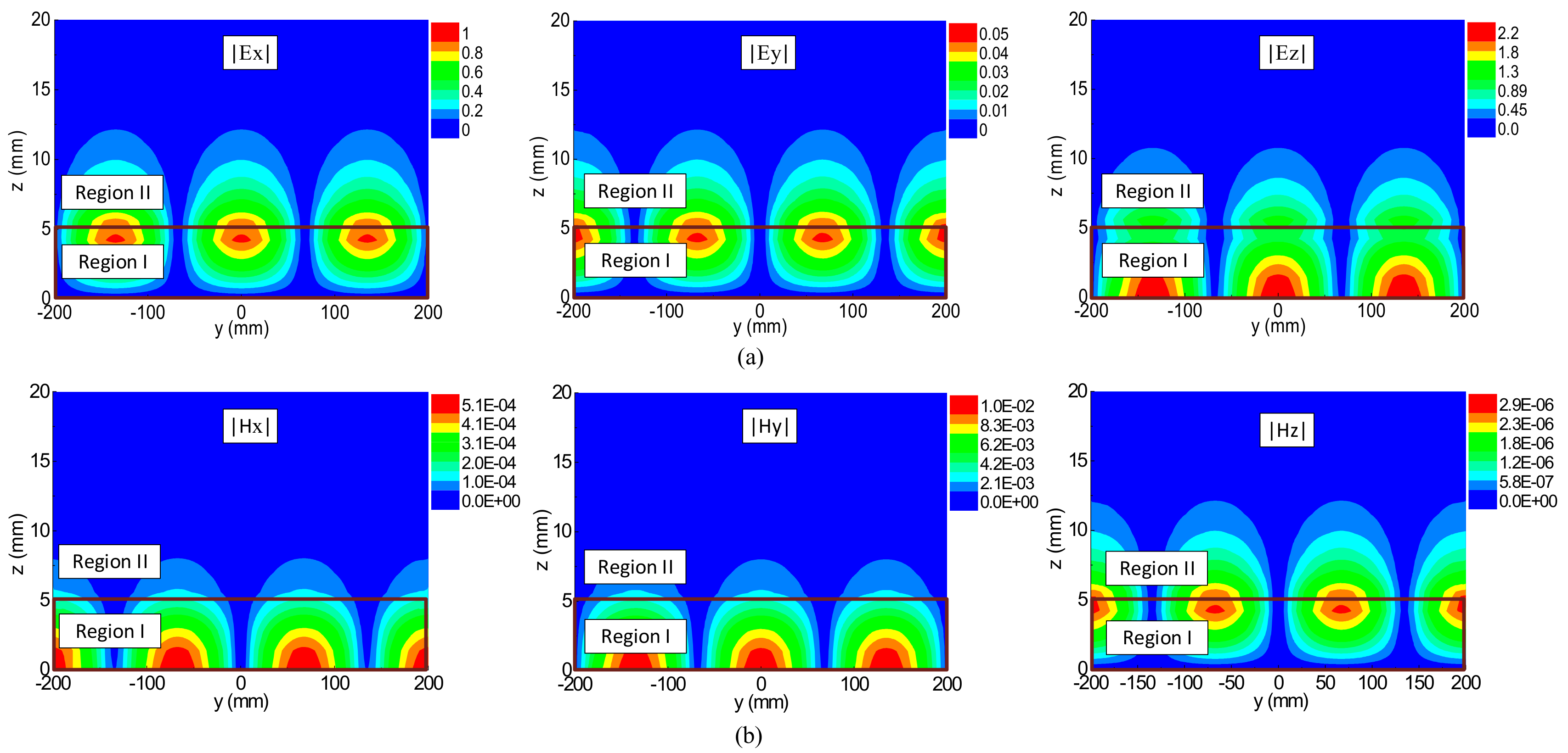
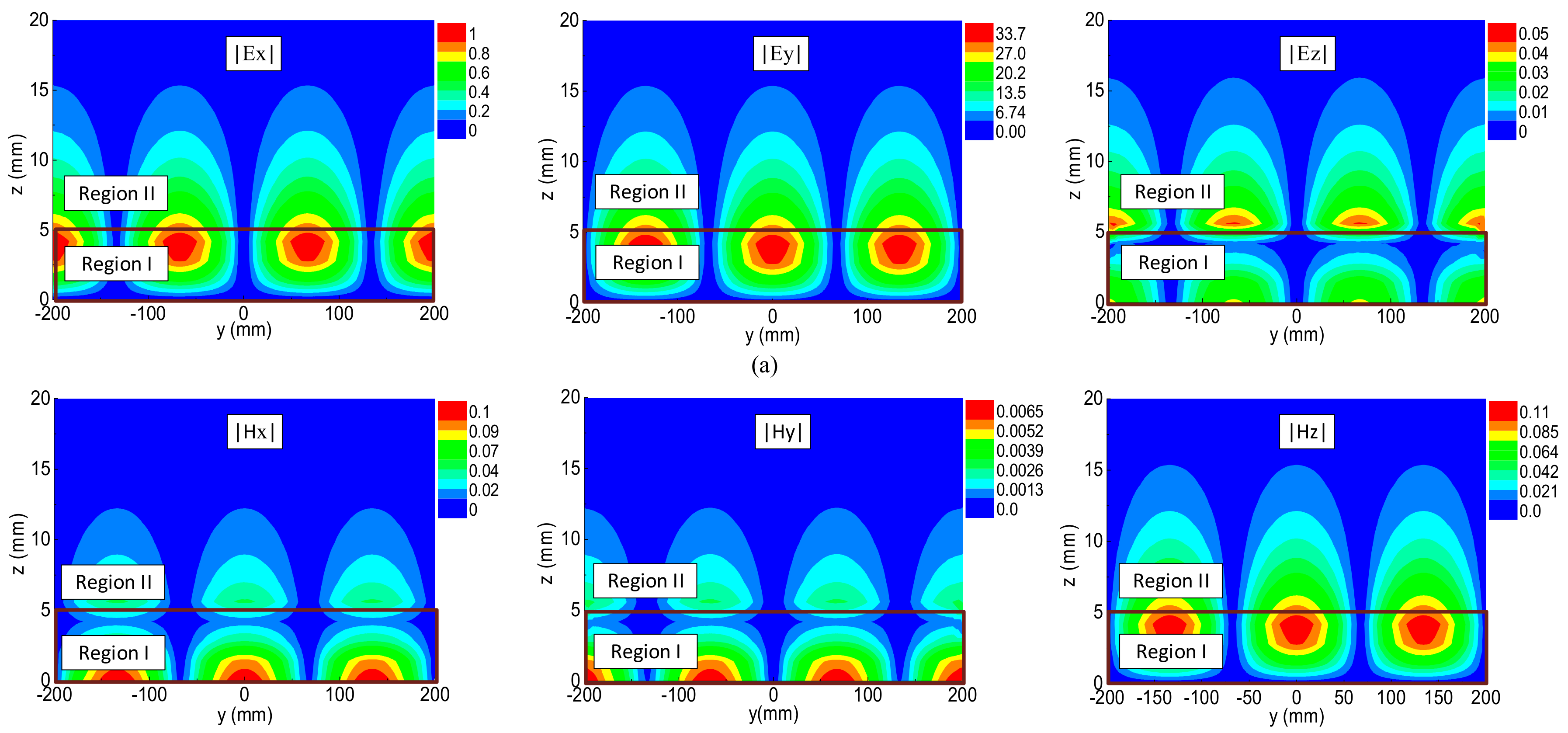
3.3. Field Distributions of Surface Waves

The field distributions of surface waves propagating on a finite-width grounded dielectric slab are examined in this section. For instance, we use an anisotropic slab with ε_x = 2.95, ε_y = 2.89, ε_z = 2.45, and μ_x = μ_y = μ_z = 1. The slab width is = 400 mm. The height of the slab is t = 5 mm (0.27λ₀ at calculated frequency f = 16 GHz). By substituting the values β_x, R_y, R_oy, k_z, k_oz, and r₁ obtained from Equations (19)–(21) and (36)–(38) into Equations (7)–(14) and (24)–(35), the field distributions in all of the regions can be obtained. Based on Figure 3, it is known that when the slab thickness is 0.27λ₀, quasi-TM₀, and quasi-TE₁ surface wave modes are excited. Figure 6 shows the distributions of E- and H-field components of the quasi-TM₀ mode on the y-z cut-plane at x = 0 mm in Regions I and II. It should be mentioned that the magnitude of E-field component along the x direction |E_x| is normalized, and the magnitudes of other components are then obtained accordingly. Based on the field distributions of the quasi-TM₀ mode, the following phenomena are observed: (1) Most fields are trapped inside the slab and bound onto the interface at z = 5 mm. When it is away from the interface, the field decay rapidly; (2) Due to the finite width of the slab, the fields non-uniformly distribute along the y direction; (3) Figure 6a shows that for the E-field components, |E_x| and |E_z| are much larger than |E_y|; Figure 6b indicates that for the H-field components, |H_x| and |H_z| are very small compared to |H_y|; (4) On the ground plane at t = 0, the tangential E-fields |E_x| and |E_y| are zero, while the normal component |E_z| is strong. On the other hand, for the H-fields, |H_x| and |H_y| are maximum, while |H_z| is zero when t = 0.

In addition, the field distributions of quasi-TE₁ mode on the y-z cut-plane at x = 0 mm are plotted in Figure 7. Several similar phenomena are observed when compared to Figure 6. However, contrary to the quasi-TM₀ mode, it is seen from Figure 7a that the E-field components of quasi-TE₁ mode |E_x| and |E_z| are small as compared to |E_y|. While for the H-field distributions in Figure 7b, |H_x| and |H_z| are much larger than |H_y|. These reasonable observations further prove the reliability of our proposed method. It is also expected that the proposed method is very promising for analyzing other higher-order surface wave modes for a thicker slab.

4. Conclusions

In conclusion, we have proposed a method to analyze the surface waves propagating on grounded anisotropic slab. Different from most open literatures, which generally assume that the fields of surface waves uniformly distribute along the transverse direction of the infinitely large grounded slab, we have thoroughly considered the field variations in the direction transverse to the wave propagation direction, and the corresponding propagation characteristics of surface waves have been derived on the basis of boundary conditions and Maxwell’s equations. Three different methods have been employed to analyze the surface waves on grounded anisotropic slab as well as to validate our derivations. The effects of the relative permittivity tensor on the propagation characteristics of surface waves have been also numerically studied. In addition, the field distributions of surface waves have been examined with the aid of the proposed method. More importantly, our method takes into account the finite-width grounded slab with the fields non-uniformly distributing along the transverse direction of the slab, which is more suitable for practical engineering.

References

1. Dyakonov, M.I. New type of electromagnetic wave propagating at an interface. Sov. Phys. JETP 1988, 67, 714–716. [Google Scholar]
2. Artigas, D.; Torner, L. Dyakonov surface waves in photonic metamaterials. Phys. Rev. Lett. 2005, 94, 013901. [Google Scholar] [CrossRef] [PubMed]
3. Chen, S.; Shen, Z.; Wu, W. Analysis of dyakonov surface waves existing at the interface of an isotropic medium and a conductor-backed uniaxial slab. J. Opt. Soc. Am. A 2014, 31, 1923–1930. [Google Scholar] [CrossRef] [PubMed]
4. Pozar, D.M. Microwave Engineering, 3rd ed.; Wiley: New York, NY, USA, 2005. [Google Scholar]
5. Liu, S.H.; Liang, C.H.; Ding, W.; Chen, L.; Pan, W.T. Electromagnetic wave propagation through a slab waveguide of uniaxially anisotropic dispersive metamaterial. Prog. Electromagn. Res. 2007, 76, 467–475. [Google Scholar] [CrossRef]
6. Nevels, R.D.; Michalski, K.A. On the behavior of surface plasmons at a metallo-dielectric interface. J. Lightware Technol. 2014, 32, 3299–3305. [Google Scholar] [CrossRef]
7. Smith, D.R.; Schurig, D. Electromagnetic wave propagation in media with indefinite permittivity and permeability tensors. Phys. Rev. Lett. 2003, 90, 077405. [Google Scholar] [CrossRef] [PubMed]
8. Yan, W.; Shen, L.; Ran, L.; Kong, J.A. Surface modes at the interfaces between isotropic media and indefinite media. J. Opt. Soc. Am. A 2007, 24, 530–535. [Google Scholar] [CrossRef]
9. Volakis, J.L. Antenna Engineering Handbook, 4th ed.; McGraw-Hill: New York, NY, USA, 2007. [Google Scholar]
10. Knoesen, A.; Gaylord, T.K.; Moharam, M.G. Hybrid guided modes in uniaxial dielectric planar waveguides. J. Lightware Technol. 1988, 6, 1083–1104. [Google Scholar]
11. Maldonado, T.A.; Gaylord, T.K. Hybrid guided modes in biaxial planar waveguides. J. Lightware Technol. 1996, 14, 486–499. [Google Scholar] [CrossRef]
12. Seshadri, S.R.; Pickard, W.F. Surface waves on an anisotropic plasma sheath. IEEE Trans. Microw. Theory Tech. 1964, 12, 529–541. [Google Scholar] [CrossRef]
13. Engheta, N.; Pelet, P. Surface waves in chiral layers. Opt. Lett. 1991, 16, 723–725. [Google Scholar]
14. Rockstuhl, C.; Lederer, F. Intrinsic surface and bulk defected modes in quasi-periodic photonic crystals. J. Lightware Technol. 2007, 25, 2299–2305. [Google Scholar] [CrossRef]
15. Attwood, S.S. Surface-wave propagation over a coated plane conductor. J. Appl. Phys. 1951, 22, 504–509. [Google Scholar] [CrossRef]
16. Liu, S.; Chen, L.; Liang, C. Guided modes in a grounded slab waveguide of uniaxially anisotropic left-handed material. Microw. Opt. Technol. Lett. 2007, 49, 1644–1648. [Google Scholar] [CrossRef]
17. Baccarelli, P.; Burghignoli, P.; Frezza, F.; Galli, A.; Lampariello, P.; Lovat, G.; Paulotto, S. Fundamental modal properties of surface waves on metamaterial grounded slabs. IEEE Trans. Microw. Theory Tech. 2005, 53, 1431–1442. [Google Scholar] [CrossRef]
18. Chen, Z.; Shen, Z. Wideband flush-mounted surface wave antenna of very low profile. IEEE Trans. Antennas Propag. 2015, 63, 2430–2438. [Google Scholar] [CrossRef]
19. Jiang, Z.H.; Wu, Q.; Brocker, D.E.; Sieber, P.E.; Werner, D.H. A low-profile high-gain substrate-integrated waveguide slot antenna enabled by an ultrathin anisotropic zero-index metamaterial coating. IEEE Trans. Antennas Propag. 2014, 62, 1173–1184. [Google Scholar] [CrossRef]
20. Jiang, Z.H.; Wu, Q.; Werner, D.H. Demonstration of enhanced broadband unidirectional electromagnetic radiation enabled by a subwavelength profile leaky anisotropic zero-index metamaterial coating. Phys. Rev. B 2012, 86, 125131. [Google Scholar] [CrossRef]
21. Olyphant, M. Measuring anisotropy in microwave substrates. In Proceedings of the 1979 IEEE MTT-S International Microwave Symposium Digest, Orlando, FL, USA, 30 April–2 May 1979. [Google Scholar]
22. Marcatili, E.A.J. Dielectric rectangular waveguide and directional coupler for integrated optics. Bell Syst. Tech. J. 1969, 48, 2071–2102. [Google Scholar] [CrossRef]
Figure 1. Surface waves on the interface of air region and grounded anisotropic slab with infinite length in x and y directions.
Applsci 08 00102 g001
Figure 2. Surface waves on the interface of air region and grounded anisotropic slab with finite width: (a) Perspective view; and, (b) Cross-section view.
Applsci 08 00102 g002
Figure 3. Comparison of βx/k0 as a function of slab thickness t/λ0 for grounded dielectric slab, (a) anisotropic slab with εx = 2.95, εy = 2.89, εz = 2.45 and μx = μy = μz = 1; (b) isotropic slab with εx = εy = εz = 2.45, μx = μy = μz = 1. (a = ∞ for Ry = 0, 2a = 37.5 mm for Ry ≠ 0).
Applsci 08 00102 g003
Figure 4. Effects of slab width on (a) βx/k0 and (b) |βx/Ry| as a function of slab thickness for grounded anisotropic slab. (εx = 2.95, εy = 2.89, εz = 2.45, μx = μy = μz = 1).
Applsci 08 00102 g004
Figure 5. Effects of (a); (d) εx; (b); (e) εy; and (c,f) εz on βx/k0 and |βx/Ry| as a function of slab thickness for grounded anisotropic slab with slab width of 2a = 56.25 mm.
Applsci 08 00102 g005
Figure 6. Distributions of (a) E-field and (b) H-field components of quasi-TM0 mode when surface wave is propagation on the finite-width grounded anisotropic slab. (y-z cut-plane at x = 0 mm, t = 5 mm, 2a = 400 mm, εx = 2.95, εy = 2.89, εz = 2.45, μx = μy = μz = 1, f = 16 GHz).
Applsci 08 00102 g006
Figure 7. Distributions of (a) E-field and (b) H-field components of quasi-TE1 mode when surface wave is propagation on the finite-width grounded anisotropic slab. (y-z cut-plane at x = 0 mm, t = 5 mm, 2a = 400 mm, εx = 2.95, εy = 2.89, εz = 2.45, μx = μy = μz = 1, f = 16 GHz).
Applsci 08 00102 g007