Audlet Filter Banks: A Versatile Analysis/Synthesis Framework Using Auditory Frequency Scales

Featured Application

The proposed framework is highly suitable for audio applications that require analysis–synthesis systems with the following properties: stability, perfect reconstruction, and a flexible choice of redundancy.

Abstract

Many audio applications rely on filter banks (FBs) to analyze, process, and re-synthesize sounds. For these applications, an important property of the analysis–synthesis system is the reconstruction error; it has to be minimized to avoid audible artifacts. Other advantageous properties include stability and low redundancy. To exploit some aspects of auditory perception in the signal chain, some applications rely on FBs that approximate the frequency analysis performed in the auditory periphery, the gammatone FB being a popular example. However, current gammatone FBs only allow partial reconstruction and stability at high redundancies. In this article, we construct an analysis–synthesis system for audio applications. The proposed system, referred to as Audlet, is an oversampled FB with filters distributed on auditory frequency scales. It allows perfect reconstruction for a wide range of FB settings (e.g., the shape and density of filters), efficient FB design, and adaptable redundancy. In particular, we show how to construct a gammatone FB with perfect reconstruction. Experiments demonstrate performance improvements of the proposed gammatone FB when compared to current gammatone FBs in terms of reconstruction error and stability, especially at low redundancies. An application of the framework to audio source separation illustrates its utility for audio processing.

1. Introduction

Time-frequency (TF) transforms like the short-time Fourier or wavelet transforms play a major role in audio signal processing. They allow any signal to be decomposed into a set of elementary functions with good TF localization and perfect reconstruction is achieved if the transform parameters are chosen appropriately (e.g., [1,2]). The result of a signal analysis is a set of TF coefficients, sometimes called sub-band components, that quantifies the degree of similarity between the input signal and the elementary functions. In applications, TF transforms are used to perform sub-band processing, that is, to modify the sub-band components and synthesize an output signal. De-noising techniques [3,4], for instance, analyze the noisy signal, estimate the TF coefficients associated with noise, delete them from the set of TF coefficients, and synthesize a clean signal from the set of remaining TF coefficients. Lossy audio codecs like MPEG-2 Layer III, known as MP3 [5], or advanced audio coding (AAC) [6,7] quantize the sub-bands with a variable precision in order to reduce the digital size of audio files. In audio transformations like time-stretching or pitch-shifting [8,9], the phases of sub-band components are processed to ensure a proper phase coherence. As a last example, applications of audio source separation [10,11,12] or polyphonic transcriptions of music [13] rely on the non-negative matrix factorization scheme: the set of TF coefficients is factorized into several matrices that correspond to various sources present in the original signal. Each source can then be synthesized from its matrix representation. In these applications, the short-time Fourier transform (STFT) is mostly used, although modified discrete cosine transforms (MDCTs) are usually preferred in audio codecs.

Because sub-band processing may introduce audible distortions in the reconstructed signal, important properties of the analysis–synthesis system include stability (i.e., the coefficients are bounded if and only if the input signal is bounded), perfect reconstruction (i.e., the reconstruction error is only limited by numerical precision when no sub-channel processing is performed), resistance to noise, and aliasing suppression in each sub-band (e.g., [14,15] Chap. 10). Furthermore, in all applications, a low redundancy (i.e., a redundancy between 1 and 2) lowers the computational costs.

TF transforms are usually implemented as filter banks (FBs) where the set of analysis filters defines the elementary functions and the set of synthesis filters allows signal reconstruction. The TF concentration of the filters together with the downsampling factors in the sub-bands define the TF resolution and redundancy of the transform. FBs come in various flavors and have been extensively treated in the literature (e.g., [16,17,18,19]). The mathematical theory of frames constitutes an interesting alternative background for the interpretation and implementation of FBs (e.g., [20,21,22]). Gabor frames (sampled STFT [2,23]), for instance, are widespread in audio signal processing.

For certain applications, such as audio coding [5,6,7], audio equalizers [24], speech processing [25], perceptual sparsity [26,27], or source separation [11,12,28,29], exploiting some aspects of human auditory perception in the signal chain constitutes an advantage. One of the most exploited aspects of the auditory system is the auditory frequency scale, which is a simple means to approximate the frequency analysis performed in the auditory system [30]. Generally, the auditory system is a complex and in many aspects nonlinear system (for a review see, e.g., [31]). Its description ranges from simple collections of linear symmetric bandpass filters [32] through collections of asymmetric and compressive filters [33] to sophisticated models of nonlinear wave propagation in the cochlea [34]. Because nonlinear systems may complicate the inversion of the signal processing chain (e.g., [35,36]), linear approximations of the auditory system are often preferred in audio applications. In particular, gammatone filters approximate well the auditory periphery at low to moderate sound pressure levels [37,38] and are easy to implement as FIR or IIR filters [32,39,40,41,42,43].

Various analysis–synthesis systems based on gammatone FBs have been proposed for the purpose of audio applications (e.g., [35,39,40,44]). However, these systems do not satisfy all requirements of audio applications as, even at high redundancies, they only achieve a reconstruction error described as “barely audible”. This error becomes clearly audible at low redundancies. In other words, these systems do not achieve perfect reconstruction. To our knowledge, a general recipe for constructing a gammatone FB with perfect reconstruction at redundancies close to and higher than one has not been published yet.

In this article, we describe a general recipe for constructing an analysis–synthesis system using a non-uniform oversampled FB with filters distributed on an arbitrary auditory frequency scale, enabling perfect reconstruction at arbitrary redundancies. The resulting framework is named “Audlet” for audio processing and auditory motivation. The proposed approach follows the theoretical foundation of non-stationary Gabor frames [20,45] and their application to TF transforms with a variable TF resolution [46,47,48]. This report extends the work reported in [20] (Section 5.1) by providing a full theoretical and practical development of the Audlet.

The manuscript is organized as follows. The next section briefly recalls the basics of non-uniform FBs, frames, and auditory frequency scales. Section 3 describes the theoretical construction of the Audlet framework. The practical implementation issues are discussed in Section 4 and Section 5 evaluates important properties and capabilities of the framework.

2. Preliminaries

2.1. Notations and Definition

In the following, we consider signals in ${\ell }_2(\mathbb{Z})$ as samples of a continuous signal with sampling frequency $f_s$, with the Nyquist frequency of $f_N=f_s/2$. We denote the normalized frequency by $\xi =f/f_s$, i.e., the interval $\left[0,f_N\right]$ corresponds to $\left[0,1/2\right]$. The inner product of two signals $x,y$ is $〈x,y〉={\sum }_{n}x\left[n\right]·y\left[n\right]$ and the energy of a signal is defined from the inner product as $\left|\right|x\left|\right|=〈x,x〉$. The floor, ceiling, and rounding operators are $\lfloor ·\rfloor ,\lceil ·\rceil$, and $\lfloor ·\rceil$, respectively. We denote the z-transform by $\mathcal{Z}$: $x\left[n\right]\mapsto X(z)$. By setting $z=e^{2i\pi \xi }$ for $\xi \in (-1/2,1/2]$, the z-transform equals the discrete-time Fourier transform ($\mathrm{DTFT}$). Note that the frequency domain associated to the $\mathrm{DTFT}$ is circular and therefore, the interval $(-1/2,1/2]$ is considered circularly, i.e., $\xi \in \mathbb{R}$ is identified with $\xi -\lfloor \xi \rceil \in (-1/2,1/2]$. The same applies for $(-f_N,f_N]$. Since we exclusively consider real-valued signals we deal with symmetric $\mathrm{DTFT}$s, which allows us to process only the positive-frequency range. Finally, we denote the complex conjugation by an overbar, e.g., $\overline{H}$.

2.2. Filter Banks and Frames

The general structure of a non-uniform analysis FB is presented in Figure 1 (e.g., [17]). It is a collection of $K+1$ analysis filters $H_k(z)$, where $H_k(z)$ is the z-transform of the impulse response $h_k\left[n\right]$ of the filter, and downsampling factors $d_k,k\in \left\{0\dots K\right\},$ that divides a signal x into a set of $K+1$ sub-band components $y_k$, where

$$y_k{\left[n\right]=\downarrow }_{d_k}\left\{h_k\ast x\right\}\left[n\right].$$

(1)

The special case where all downsampling factors are identical, i.e., $d_k=D\forall k\in \left\{0\dots K\right\}$, is referred to as a uniform FB.

By analogy, a synthesis FB is a collection of $K+1$ upsampling factors $d_k$ and synthesis filters $G_k(z)$ (see Figure 2) that recombines the sub-band components $y_k$ into an output signal $\tilde{x}$ according to

$$\tilde{x}\left[n\right]=2\Re \left(\sum _{k=0}^K\left(g_k{\ast \uparrow }_{d_k}\left\{y_k\right\}\right)\left[n\right]\right),$$

(2)

where ℜ, denoting the real part, and the factor of 2 are a consequence of considering the positive frequency range only.

A synthesis FB can be generalized to a synthesis system (shown in Figure 3), which is a linear operator $\mathcal{S}$ that takes as an input sub-band components $y_k$ and yields an output sequence $\tilde{x}$. For the synthesis operation, we use the notation $\tilde{\mathcal{S}}(·,{(G_k,d_k)}_k)$, where ${(G_k,d_k)}_k$ is the synthesis FB. An analysis FB is invertible or allows for perfect reconstruction if there exists a synthesis system $\mathcal{S}$ that recovers x from the sub-band components $y_k$ without error, i.e., $\tilde{x}=x$ for all $x\in {\ell }_2(\mathbb{Z})$. In other terms, the analysis–synthesis system $\left({(H_k,d_k)}_k,\mathcal{S}\right)$ has the perfect reconstruction property. In practice, the implementation of that operation might introduce errors of the order of numerical precision.

We use the mathematical theory of frames in order to analyze and design perfect reconstruction FBs (e.g., [20,21,22]). A frame over the space of finite energy signals ${\ell }_2(\mathbb{Z})$ is a set of functions spanning the space in a stable fashion. Consider a signal x and an analysis FB ${(H_k,d_k)}_k$ yielding $y_k$. Then, an FB constitutes a frame if and only if $0<A\le B<\infty$ exist such that

$${A\parallel x\parallel }^2\le \sum _k\parallel y_k{\parallel }^2\le B{\parallel x\parallel }^2,\forall x\in {\ell }^2(\mathbb{Z})$$

(3)

where A and B are called the lower and upper frame bounds of the system, respectively. The existence of A and B guarantees the invertibility of the FB. Several numerical properties of an FB can be derived from the frame bounds. In particular, the ratio $\sqrt{B/A}$ corresponds to the condition number [49] of the FB, i.e., it determines the stability and reconstruction error of the system. Furthermore, the ratio B/A characterizes the overall frequency response of the FB. A ratio $B/A=1$, for instance, means a perfectly flat frequency response. This is often desired in signal processing because, in that particular case, the analysis and synthesis FB are the same. Specifically, the synthesis filters are obtained by time-reversing the analysis filters, i.e., $G_k(z)={\overline{H}}_k(z)$.

The frame bounds A and B correspond to the infinimum and supremum, respectively, of the eigenvalues of the operator $\tilde{\mathcal{S}}(\mathcal{A}(·,{(H_k,d_k)}_k),{(H_k,d_k)}_k)$ associated with the system ${(H_k,d_k)}_k$. In practice, these eigenvalues can be computed using iterative methods (see Section 3.2 and Section 3.3).

2.3. Auditory Frequency Scales

An important aspect of the auditory system to consider in auditory-motivated analysis is the frequency-to-place transformation that occurs in the cochlea. Briefly, when a sound reaches the ear it produces a vibration pattern on the basilar membrane. The position and width of this pattern along the membrane depend on the spectral content of the sound; high-frequency sounds produce maximum excitation at the base of the membrane, while low-frequency sounds produce maximum excitation at the apex of the membrane. This property of the auditory system can be modeled in a first approximation as a bank of bandpass filters, named “critical bands” or “auditory filters”, whose center frequencies and bandwidths respectively approximate the place and width of excitation on the basilar membrane. The frequency and bandwidth of the auditory filters are nonlinear functions of frequency. These functions, called auditory frequency scales, are derived from psychoacoustic experiments (see e.g., [50], Chapter 3 for a review). The Bark, the equivalent rectangular bandwidth (ERB), and Mel scales are commonly used in hearing science and audio signal processing [30]. To refer to the different frequency mappings we introduce the function F: $f\to \mathrm{Scale}$ where f is frequency in Hz and $\mathrm{Scale}$ is an auditory unit that depends on the scale. The ERB rate, for instance, is [30]

$$F_{\mathrm{ERB}}(f)=9.265\ln \left(1+\frac{f}{228.8455}\right)$$

(4)

and its inverse is

$$f=F_{\mathrm{ERB}}^{-1}(F_{\mathrm{ERB}})=228.8455\left(e^{F_{\mathrm{ERB}}/9.265}-1\right).$$

(5)

The ERB (in Hz) of the auditory filter centered at frequency f is

$$B_{\mathrm{ERB}}(f)=24.7+\frac{f}{9.265}.$$

(6)

Expressions for the Bark and Mel scales are respectively provided in [51,52]. For scales that do not specify a bandwidth function, like the Mel scale, we propose the following function: $B_{\mathrm{scale}}(f)=\frac{\partial \left(F_{\mathrm{scale}}^{-1}\right)}{\partial f}(F_{\mathrm{scale}}(f))$. This ensures a proper overlap between the filters’ passband.

3. The Proposed Approach

This section describes the analysis FB and synthesis stage of the Audlet FB. The FB is entirely designed in the frequency domain, which simplifies the assessment of properties such as invertibility and the amount of aliasing. Note that the purpose of this section is to provide a mathematical framework for general FB regardless of the practical implications. The implementation of the Audlet framework is addressed separately in Section 4.

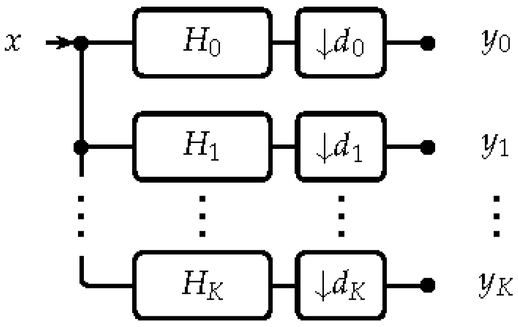
3.1. Analysis Filter Bank

The analysis FB consists of Audlet filters $H_k$, $k\in \{1,\dots ,K-1\}$, a low-pass filter $H_0$, and a high-pass filter $H_K$. In total, it consists of $K+1$ filters. The Audlet filters are defined by

$$H_k(e^{2i\pi \xi })=d_k^{\frac{1}{2}}w\left(\frac{f_s·\xi -f_k}{{\Gamma }_k}\right)k\in \{1,\dots ,K-1\}$$

(7)

where $w(\xi )$ is a prototype filter’s shape centered at frequency 0. Any symmetric or asymmetric window is an eligible w. The main condition on w is that its frequency response must decay away from 0 on both sides. The parameters ${\Gamma }_k=\beta B_{scale}(f_k)$ and $f_k$ control the bandwidth and center frequency, respectively, of the filter $H_k$. The parameter $\beta$ allows for the filter bandwidths to be compressed/expanded. Note that when $\beta \ne$ 1, the bandwidth of the filters $H_k$ deviates from the human auditory filters’ bandwidth.

To determine K and construct the sets $\left\{f_k\right\}$ and $\left\{{\Gamma }_k\right\}$, the first step consists in choosing an essential frequency range $[f_{\min },f_{\max }]\subseteq [0,f_N]$, a frequency mapping $F_{\mathrm{Scale}}$, and a filter density $V\in {\mathbb{R}}^{+}$ of filters per $\mathrm{Scale}$ unit. The set $\left\{d_k\right\}$ is considered arbitrary for now. An optimal choice of downsampling factors $d_k$ is provided in Section 3.1.3.

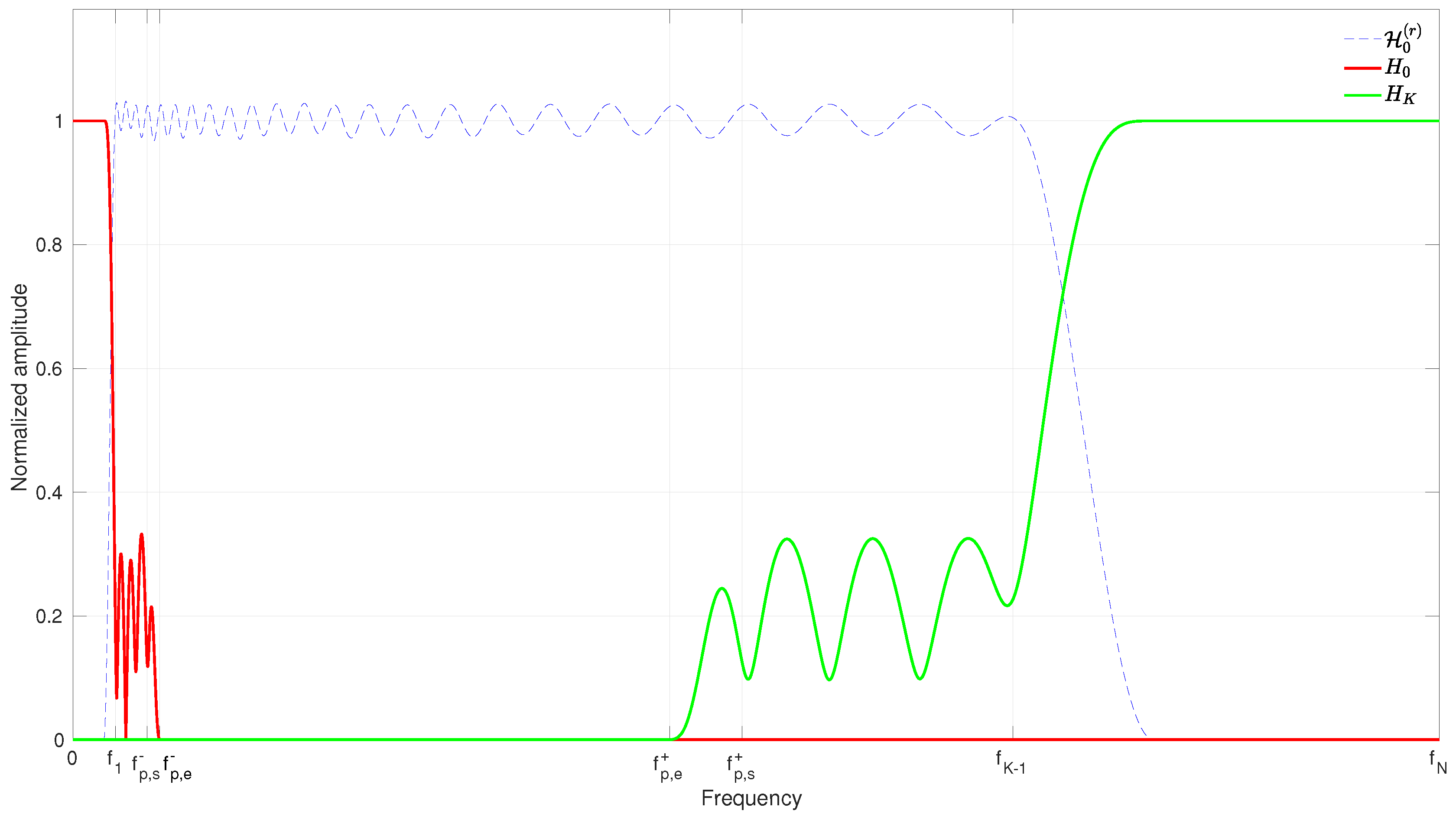
3.1.1. Construction of the Set $\left\{f_k\right\}$

The center frequency $f_1$ is given by

$$f_1=\max \{f_{\min },F_{\mathrm{Scale}}^{-1}(1/V)\}$$

(8)

and the subsequent $f_k$’s are obtained iteratively by

$$f_k=F_{\mathrm{Scale}}^{-1}(F_{\mathrm{Scale}}(f_1)+(k-1)/V).$$

(9)

The iteration is processed as long as $f_k\le f_{\max }$ and $f_k<f_N$, resulting in $K-1$ filters, with K determined by

$$\begin{array}{c}\hfill K=\min \{\underset{k\in \mathbb{N}}{argmax}\left(\frac{k-1}{V}\le F_{\mathrm{Scale}}(f_{\max })-F_{\mathrm{Scale}}(f_1)\right),\\ \hfill \underset{k\in \mathbb{N}}{argmax}\left(\frac{k-1}{V}<F_{\mathrm{Scale}}(f_N)-F_{\mathrm{Scale}}(f_1)\right)\}.\end{array}$$

Note that $f_{\max }$ should be slightly higher than the highest frequency of interest in the analyzed signals. Finally, $f_0=0$ and $f_K=f_N$. At this stage, the “restricted” frequency response of the FB (i.e, restricted to the filters $H_1,\cdots ,H_{K-1}$) is given by

$${\mathcal{H}}_0^{(r)}(\xi )={\widetilde{{\mathcal{H}}_0}}^{(r)}(\xi )+\overline{{\widetilde{{\mathcal{H}}_0}}^{(r)}(-\xi )},\mathrm{with}$$

$${\widetilde{{\mathcal{H}}_0}}^{(r)}(\xi ):=\sum _{k=1}^{K-1}{d}_k^{-1/2}{\left|H_k(e^{2\pi i\xi })\right|}^2,\mathrm{for}\mathrm{all}\xi \in (-1/2,1/2].$$

To obtain a perfect reconstruction system, the frequency response of the system should optimally cover the frequency range $[0,f_N]$. However, this may not be the case for ${\widetilde{{\mathcal{H}}_0}}^{(r)}(\xi )$ because the amplitude of the filter $H_1$ (and/or $H_{K-1}$) may vanish at frequencies between 0 and $f_1$ (resp., between $f_{K-1}$ and $f_N$). To circumvent this problem, a low-pass filter $H_0$ and high-pass filter $H_K$ are included.

3.1.2. Construction of $H_0$ and $H_K$

The purpose of the filters $H_0$ and $H_K$ is to stabilize the FB response ${\mathcal{H}}_0$ by compensating for the potentially low amplitude of ${\mathcal{H}}_0^{(r)}(\xi )$ in the range $[0,f_1[\cup ]f_{K-1},f_N]$. While the content in the frequency bands 0 and K might carry some perceptually relevant information, most applications will not modify the corresponding coefficients. Consequently, it is crucial that $H_0$ and $H_K$ are mostly concentrated outside $[f_1,f_{K-1}]$, but their time domain behavior is only of secondary importance. Nonetheless, we propose a construction that retains some smoothness in frequency and thus, by Fourier duality, $h_0$ and $h_K$ have appropriate decay.

There is no canonical method that provides optimal compensation and time localization for any valid set of Audlet parameters. In [46], for instance, plateau functions with raised cosine flanks were proposed. This method might result in additional ripples in ${\mathcal{H}}_0$ if w is not a raised-cosine window. Alternatively, in [47], $H_0$ and $H_K$ were constructed from a set of virtual filters extending the FB beyond $[f_1,f_{K-1}]$. An adaptation of this method to the Audlet framework is unnecessarily complex and unintuitive. Instead, we propose the following. We define

$$M=\underset{\xi \in [0,1/2]}{max}{\mathcal{H}}_0^{(r)}(\xi )\mathrm{and}{\mathcal{H}}_{\mathrm{inv}}^{(r)}=\sqrt{{(M-{\mathcal{H}}_0^{(r)})}_{+}}.$$

The function ${\mathcal{H}}_{\mathrm{inv}}^{(r)}$ is nonnegative and has at least the same differentiability as w (taking the positive part ${(·)}_{+}$ is only necessary in the special cases considered in the remark below). However, any ripples in ${\mathcal{H}}_0^{(r)}$ replicate in ${\mathcal{H}}_{\mathrm{inv}}^{(r)}$. To reduce this rippling effect and introduce strict band-limitation of $H_0$ and $H_K$, we multiply ${\mathcal{H}}_{\mathrm{inv}}^{(r)}$ with appropriately localized plateau functions $P_0$ and $P_K$. Assume that $f_{p,s}^{-},f_{p,e}^{-},f_{p,s}^{+},f_{p,e}^{+}\in (0,f_N)$ are chosen such that $f_1<f_{p,s}^{-}<f_{p,e}^{-}<f_{p,s}^{+}<f_N$ and $f_1<f_{p,s}^{-}<f_{p,e}^{+}<f_{p,s}^{+}<f_N$ and let

$$P_0(\xi )=\left\{\begin{array}{cc}1/\sqrt{2}\hfill & \mathrm{if}\xi f_s\in (-f_{p,s}^{-},f_{p,s}^{-})\hfill \\ cos\left(\pi \frac{\left|\xi \right|f_s-f_{p,s}^{-}}{f_{p,e}^{-}-f_{p,s}^{-}}\right)/\sqrt{2}\hfill & \mathrm{if}\left|\xi \right|f_s\in [f_{p,s}^{-},f_{p,e}^{-}]\hfill \\ 0\hfill & \mathrm{elsewhere},\hfill \end{array}\right.$$

and

$$P_K(\xi )=\left\{\begin{array}{cc}1/\sqrt{2}\hfill & \mathrm{if}\xi f_s\in (-f_N,-f_{p,s}^{+}]\cup (f_{p,s}^{+},f_N]\hfill \\ 1/\sqrt{2}-cos\left(\pi \frac{\left|\xi \right|f_s-f_{p,s}^{+}}{f_{p,s}^{+}-f_{p,e}^{+}}\right)/\sqrt{2}\hfill & \mathrm{if}\left|\xi \right|f_s\in [f_{p,e}^{+},f_{p,s}^{+}]\hfill \\ 0\hfill & \mathrm{elsewhere}.\hfill \end{array}\right.$$

The frequency $f_{p,s}^{-}$ (resp. $f_{p,s}^{+}$) defines the width of the plateau in $P_0$ (resp. $P_K$). The region $[f_{p,s}^{-},f_{p,e}^{-}]$ ($[f_{p,e}^{+},f_{p,s}^{+}]$) defines the transition area of $P_0$ ($P_K$) (see Figure 4). The filters $H_0$ and $H_K$ are finally defined by their DTFTs as

$$H_0(e^{2\pi i(·)})=P_0·{\mathcal{H}}_{\mathrm{inv}}^{(r)},\mathrm{and}{H}_K(e^{2\pi i(·)})=P_K·{\mathcal{H}}_{\mathrm{inv}}^{(r)}.$$

(10)

We propose selecting $0<{\kappa }_1<{\kappa }_2$, such that $F_{\mathrm{Scale}}(f_{K-1})-F_{\mathrm{Scale}}(f_1)\ge {\kappa }_1+{\kappa }_2$ and fix

$$f_{p,s}^{-}=F_{\mathrm{Scale}}^{-1}(F_{\mathrm{Scale}}(f_1)+{\kappa }_1),f_{p,e}^{-}=F_{\mathrm{Scale}}^{-1}(F_{\mathrm{Scale}}(f_1)+{\kappa }_2),$$

$$f_{p,s}^{+}=F_{\mathrm{Scale}}^{-1}(F_{\mathrm{Scale}}(f_{K-1})-{\kappa }_1),f_{p,e}^{+}=F_{\mathrm{Scale}}^{-1}(F_{\mathrm{Scale}}(f_{K-1})-{\kappa }_2).$$

This choice ensures that $P_0^2+P_K^2\le 1$, preventing overcompensation, and is properly adapted to the scale used. By default, we set ${\kappa }_1=3/V,{\kappa }_2=4/V$, such that $f_{p,s}^{-}=f_4,f_{p,e}^{-}=f_5,f_{p,s}^{+}=f_{K-4},f_{p,e}^{+}=f_{K-5}$. The intuition here is that from $f_4$ (resp. $f_{K-4}$) onward, the restricted FB response ${\mathcal{H}}_0^{(r)}$ is expected to be stable already, and that the size of the transition area ensures a sufficiently smooth roll-off. It should be noted that, although the filters proposed above are chosen to be strictly band-limited, a similar construction with time-limited, but only approximately band-limited, filters is also conceivable, by smoothly truncating $h_0,h_K$ instead of $H_0,H_K$.

Remark 1.

The choice of raised cosine transition areas provides continuously differentiable $P_0,P_K$. If additional decay of $h_0,h_K$ is desired, the construction of a compactly supported plateau function of arbitrary differentiability is standard, e.g., through convolution of a characteristic function with a smooth function. There are some corner cases in which one or both of the compensation filters $h_0,h_K$ are unnecessary, namely if $f_1$ is very close to 0 (resp. $f_{K-1}$ to $f_N$). In that case the maximum M should be computed over the interval $[f_1/f_s,1/2]$ (resp. $[0,f_{K-1}/f_s]$) and we set $H_0=0$ ($H_K=0$). A rule of thumb is if ${min}_{\xi \in [0,f_1/f_s]}{\mathcal{H}}_0^{(r)}(\xi )\ge (1-ϵ){min}_{\xi \in [f_1/f_s,f_{K-1}/f_s]}{\mathcal{H}}_0^{(r)}(\xi )$, for some $ϵ\ll 1$, then the low-pass filter $H_0$ is not required. An analogous argument is valid for $H_K$.

The total frequency response of the analysis FB (i.e., including the $K+1$ filters) is then

$${\mathcal{H}}_0(\xi ):=\widetilde{{\mathcal{H}}_0}(\xi )+\widetilde{{\mathcal{H}}_0}(-\xi ),\mathrm{with}$$

(11)

$$\widetilde{{\mathcal{H}}_0}(\xi ):=\sum _{k=0}^K{d}_k^{-1}{\left|H_k(e^{2\pi i\xi })\right|}^2,\mathrm{for}\mathrm{all}\xi \in (-1/2,1/2].$$

and the redundancy of the FB is

$$R=d_0^{-1}+2\sum _{k=1}^{K-1}{d}_k^{-1}+d_K^{-1}.$$

(12)

The factor of 2 stems from the fact that coefficients in the 1-st to $(K-1)$-th sub-bands may be complex valued.

3.1.3. Construction of the Set $\left\{d_k\right\}$

Downsampling the filters’ outputs, i.e., using $d_k>1$ for some or all $k\in \{0,\dots ,K\}$, has the advantage of reducing R but introduces aliasing. The amount of aliasing can be determined from the frequency domain representation of the output signal $\tilde{X}(z)={\sum }_k\mathcal{Z}\left(g_k{\ast \uparrow }_{d_k}\left\{y_k\right\}\right)\left[n\right]$, also called the alias domain representation [16,17]. For $\xi \in (-1/2;1/2],\tilde{X}(z)$ reduces to the following ([20] Section 4)

$$\tilde{X}(e^{2i\pi \xi })=\frac{1}{D}[X(e^{2i\pi (\xi +0/D)})\cdots X(e^{2i\pi (\xi +(D-1)/D)})]{\mathcal{H}}_j(\xi )$$

(13)

where $D=\mathrm{lcm}({\left\{d_k\right\}}_k)$ and

$${\mathcal{H}}_j(\xi ):={\tilde{\mathcal{H}}}_j(\xi )+\overline{{\tilde{\mathcal{H}}}_j(-\xi )}\mathrm{with}$$

(14)

$${\tilde{\mathcal{H}}}_j(\xi )=\sum _{\begin{array}{c}k\in \{0,\dots ,K\},\\ \mathrm{s}.\mathrm{t}.j\in \frac{D}{d_k}\mathbb{Z}\end{array}}{d}_k^{-1}{H}_k(e^{2\pi i\xi })\overline{H_k(e^{2\pi i(\xi +j/D)})},$$

for all $j\in \{0,\dots ,D-1\}$. The term ${\mathcal{H}}_0$ in (14) represents the frequency response of the FB, while the terms ${\mathcal{H}}_j,j\ne 0$, represent the alias components. Thus, an alias-free system is obtained when ${\mathcal{H}}_0=C>0$ and ${\mathcal{H}}_j=0,\forall j\ne 0$. While this is not always achievable, choosing $d_k$’s to be inversely proportional to the filters’ bandwidth yields a close-to-optimal solution [19], i.e.,

$$d_k=⌊\frac{c_{bw}{f}_s}{{\Gamma }_k}⌋\mathrm{for}k=1,\dots ,K-1.$$

(15)

For a targeted redundancy $R_{\mathrm{t}}$, combining (15) and (12) while disregarding the floor operator $\lfloor ·\rfloor$ leads to

$$\begin{array}{c}\hfill c_{bw}=\frac{2}{R_{\mathrm{t}}{f}_s}\sum _{k=1}^{K-1}\beta B_{\mathrm{scale}}(f_k).\end{array}$$

(16)

Since the $H_k$ values are strictly decaying away from $f_k$ with a bandwidth of ${\Gamma }_k$, choosing $d_k$’s according to (15) ensures an even distribution of the overall aliasing across channels.

Using (15) to derive $d_0$ and $d_K$ may result in a large amount of aliasing because $H_0$ and $H_K$ may feature large plateaus depending on $f_{\min }$ and $f_{\max }$. We propose instead choosing $d_0$ and $d_K$ according to

$$\begin{array}{ccc}\hfill d_0& =& ⌊\frac{f_s}{2f_{p,s}^{-}+\frac{\beta B_{\mathrm{scale}}(f_{p,s}^{-})}{c_{bw}}}⌋\hfill \end{array}$$

(17)

$$\begin{array}{ccc}\hfill d_K& =& ⌊\frac{f_s}{2(f_N-f_{p,s}^{+})+\frac{\beta B_{\mathrm{scale}}(f_{p,s}^{+})}{c_{bw}}}⌋.\hfill \end{array}$$

(18)

Note that $R_{\mathrm{t}}$ controls the $d_k$ only for $k=1,\dots ,K-1$, while the actual redundancy R depends on all $d_k$, i.e., including $d_0$ and $d_K$. As a result, the value of R is slightly larger than $R_{\mathrm{t}}$.

3.2. Invertibility Test

Overall, the design of an Audlet analysis FB involves a set of seven parameters: the perceptual scale, frequency range $[f_{\min },f_{\max }]$, filter shape w, filter density V and bandwidth factor $\beta$, and a target redundancy $R_{\mathrm{t}}$. To check that a given parameter set results in a stable and invertible system, three methods exist:

• An eigenvalue analysis of the linear operator corresponding to analysis with ${(H_k,d_k)}_k$ followed by FB synthesis with ${(H_k,d_k)}_k$. The frame bounds A and B correspond to the smallest (infinimum) and largest (supremum) eigenvalues of the resulting operator, respectively. The largest eigenvalue can be estimated by numerical methods with reasonable efficiency but estimating the smallest eigenvalue directly is highly computationally expensive. In the next section we discuss an alternative method that consists in approximating the inverse operator and estimating its largest eigenvalue, the reciprocal of which is the desired lower frame bound A (see also Section 5 for an example frame bounds analysis).
• Computation of A and B directly from the overall FB response, i.e., verification that $0<A\le {\mathcal{H}}_0(\xi )\le B<\infty$ for some constants $A,B$ and almost every $\xi \in (-1/2,1/2]$.
• Checking of whether the overall aliasing is dominated by ${\mathcal{H}}_0$, i.e., if there exist $0<A_0\le B_0<\infty$ that satisfy

  $$A_0\le {\mathcal{H}}_0(\xi )\pm \sum _{j=1}^{D-1}\left|{\mathcal{H}}_j(\xi )\right|\le B_0,$$

  (19)

  for almost every $\xi \in [-1/2,1/2]$. This method is a straightforward application of [20] (Proposition 5). The inner term in (19) can be computed or, at least, estimated by direct computation.

While method 1 above can always be applied, the applicability of methods 2 and 3 depends on w. If w is compactly supported in the interval $[a,b]$ and $0<\frac{b-a}{{\Gamma }_{K-1}}\le f_s$, $d_k\le \frac{f_s}{(b-a){\Gamma }_k}\forall k\in \{1,\dots ,K-1\}$ (i.e., $c_{bw}\le {(b-a)}^{-1}$), $d_0\le \frac{f_s}{2f_{p,e}^{-}}$, and $d_K^{-1}\le \frac{f_s}{f_s-2f_{p,e}^{+}}$, then the alias terms ${\mathcal{H}}_j$, $j\in \{1,\dots ,D-1\}$ = 0. This setting corresponds to the painless case [53]. This is the only case when method 2 can be applied. If w has no compact support but is mostly concentrated on $[a,b]$ and decays outside, the alias terms ${\mathcal{H}}_j,j\in \{1,\dots ,D-1\}$ exist but may be small compared to ${\mathcal{H}}_0$. In that case, method 3 can be applied.

In terms of computational costs, method 1 is by far the most demanding of the three. Still, if a certain parameters set is used over a large number of analyses, this one-time investment to determine invertibility easily pays off. However, the user must still be aware of the potential inaccuracies induced by numerical eigenvalue computation.

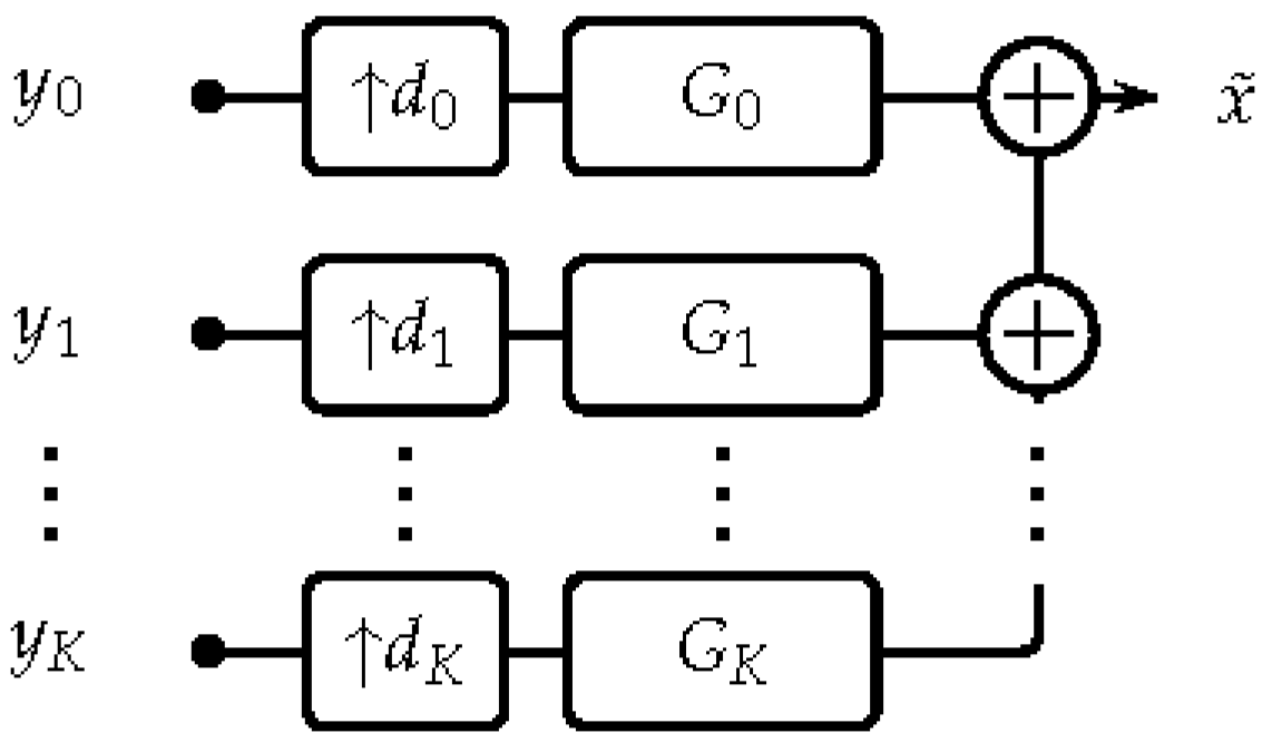
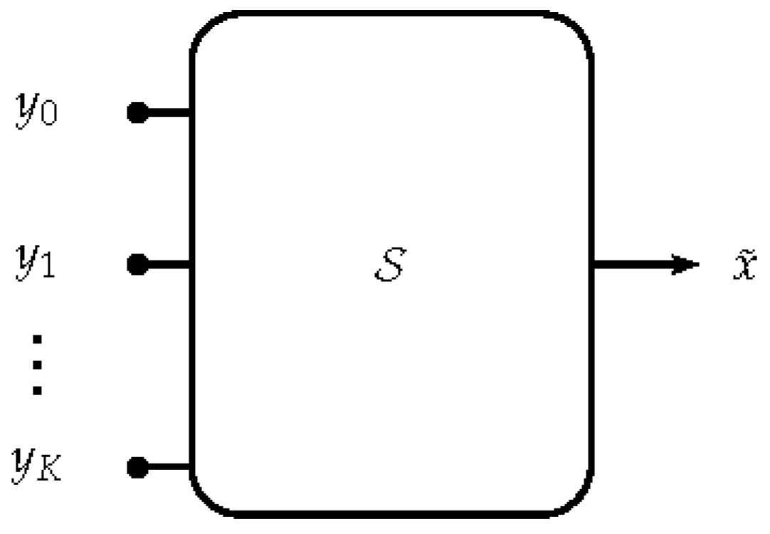
3.3. Synthesis Stage

The synthesis stage consists of a linear operator $\mathcal{S}({(y_k)}_k)$ mapping the sub-band signals $y_k$ to the output signal $\tilde{x}$ (see Figure 3) such that the input signal x is recovered. For uniform analysis FBs, i.e., $d_k=D\forall k$, the operator $\mathcal{S}$ can be structured as in Figure 2. In that case, exact dual filter $G_k$’s can be computed [54] with a factorization algorithm that generalizes [23]. The synthesis is then performed by computing $\tilde{\mathcal{S}}({(y_k)}_k,{(G_k,D)}_k)$.

For non-uniform analysis FBs, we implement $\mathcal{S}$ using a conjugate gradient (CG) iteration [49,55,56]. This is a very efficient iterative algorithm that is guaranteed to converge when ${(H_k,d_k)}_k$ forms a frame, i.e., whenever stable perfect reconstruction is possible. Given the Hermitian operator $\tilde{\mathcal{S}}(\mathcal{A}(x,{(H_k,d_k)}_k),{(H_k,d_k)}_k)$, the CG approximates the action of the inverse operator. For Hermitian operators, the CG converges monotonously to 0. In addition, for problems of size P, the CG is guaranteed to converge within P steps. In practice, convergence speed depends solely on the (potentially unknown) condition number of the linear problem at hand, which, in this case, equals $\sqrt{B/A}$. Often, it is beneficial to use a preconditioning step to improve the condition number. We propose the operator ${\mathcal{F}}^{-1}diag(1/{\mathcal{H}}_0)\mathcal{F}$ as preconditioner (see also [48,57,58]). A robust implementation of the appropriate preconditioned CG (PCG) algorithm is conceptually straightforward and was provided in [48].

In the following, we describe a heuristic variant of this PCG algorithm with asymmetric preconditioning, that enables efficient implementation even if the intermediate solutions (denoted by $x_j$ below) are only given in the time domain. Experimentally, Algorithm 1 was observed to converge in the same number of iterations as the robust implementation from [48] (divergence was observed only if the filters $H_k$ were set to uniformly distributed random noise). We denote the analysis of x with respect to the analysis FB ${(H_k,d_k)}_k$ by ${(y_k)}_k=\mathcal{A}(x,{(H_k,d_k)}_k)$. We denote the synthesis from ${(y_k)}_k$ with respect to the synthesis FB ${(G_k,d_k)}_k$ by $\tilde{x}=\tilde{\mathcal{S}}({(y_k)}_k,{(G_k,d_k)}_k)$. The composition $\tilde{x}=\tilde{\mathcal{S}}(\mathcal{A}(x,{(H_k,d_k)}_k),{(G_k,d_k)}_k)$ thus represents analysis followed by synthesis.

Algorithm 1 Synthesis by means of conjugate gradients

Initialize ${(H_k,d_k)}_k$, ${(y_k)}_k$

$x_0\in {\ell }_2(\mathbb{Z})$ (arbitrary)

$j=0$ and $\epsilon >0$ (error tolerance)

${\mathcal{H}}_0\leftarrow {\sum }_k{d}_k^{-1}{H}_k$

for $k=0,\dots ,K+1$ do

$G_k\leftarrow H_k/{\mathcal{H}}_0$

end for

$b\leftarrow \tilde{\mathcal{S}}({(y_k)}_k,{(G_k,d_k)}_k)$

$r_0\leftarrow b-\tilde{\mathcal{S}}(\mathcal{A}(x_0,{(H_k,d_k)}_k),{(G_k,d_k)}_k)$

$p_0\leftarrow r_0$

while $r_j>\epsilon$ do

$q_j\leftarrow \tilde{\mathcal{S}}(\mathcal{A}(p_j,{(H_k,d_k)}_k),{(G_k,d_k)}_k)$

$a_j\leftarrow {\left|r_j\right|}^2/\langle p_j,q_j\rangle$

$x_{j+1}\leftarrow x_j+a_j{p}_j$

$r_{j+1}\leftarrow r_j-a_j{q}_j$

$b_j\leftarrow {|r_{j+1}/r_j|}^2$

$p_{j+1}\leftarrow r_{j+1}+b_j{p}_j$

$j\leftarrow j+1$

end while

To speed up convergence we use approximate dual filters as an initial choice for $G_k$’s,

$$G_k(e^{2i\pi \xi }):=\frac{H_k(e^{2i\pi \xi })}{{\mathcal{H}}_0(\xi )}.$$

(20)

We interpret $G_k$’s as approximate dual filters because in the absence of aliasing (i.e., if ${\mathcal{H}}_j=0,\forall j\ne 0$), the application of $G_k$ exactly cancels all ripples in the frequency response ${\mathcal{H}}_0$. Hence, the analysis-synthesis system $\tilde{\mathcal{S}}(\mathcal{A}(x,{(H_k,d_k)}_k),{(G_k,d_k)}_k)$ can be interpreted as a preconditioned variant of $\tilde{\mathcal{S}}(\mathcal{A}(x,{(H_k,d_k)}_k),{(H_k,d_k)}_k)$ [48,57,58].

Note that in the painless case, evoked in Section 3.2, the operator $\tilde{\mathcal{S}}(\mathcal{A}(x,{(H_k,d_k)}_k),$ ${(G_k,d_k)}_k)$ equals the identity and thus, synthesis is performed simply by applying $\tilde{\mathcal{S}}({(y_k)}_k,{(G_k,d_k)}_k)$ once.

Although this is not apparent from the iterative inversion scheme described above, the proposed synthesis stage acts in a similar fashion to an FB. More specifically, if $D=lcm({\left\{d_k\right\}}_k)$ and ${({\tilde{H}}_j,D)}_j$ is the equivalent uniform FB associated with ${(H_k,d_k)}_k$ [16,20], then iterating the CG algorithm until convergence is equivalent to computing the FB synthesis with respect to the canonical dual FB of ${({\tilde{H}}_j,D)}_j$, which is of the form ${({\tilde{G}}_j,D)}_j$, for some sequences of filters ${({\tilde{G}}_j)}_j$ (see [21]). Since convergence is achieved within numerical precision in a small number of CG steps we can assume that the proposed synthesis system is characterized by the properties of the filters ${({\tilde{G}}_j)}_j$. We cannot easily compute those filters, but it is well known that the ratio of the optimal frame bounds $B/A$ (see Section 3.2) is closely related to the similarity of a system and its canonical dual [59]. If $B/A\approx 1$, then we can expect ${\tilde{G}}_j\approx {\tilde{H}}_j$, for all j. Since each ${\tilde{H}}_j$ is just a delayed version of some $H_k$, the time- and frequency-domain localization of the synthesis system matches that of the analysis system.

For larger values of $B/A$, the duality of ${({\tilde{H}}_j,D)}_j$ and ${({\tilde{G}}_j,D)}_j$ implies that ${({\tilde{G}}_j,D)}_j$ has to account for the discrepancies of ${({\tilde{H}}_j,D)}_j$ [59]. These considerations apply to any dual FB pair, Audlet or not. The Audlet FB is constructed in such a way that, given the prototype filter w and filter density V, the frequency response of ${(H_k,d_k)}_k$ is as flat as possible, such that the $B/A$ depends mostly on the presence of aliasing. The required aliasing compensation often implies a widening of the dual filters’ essential support and essential passband, proportional to the amount of aliasing present.

4. Implementation

4.1. Practical Issues

The general mathematical framework described in the previous section is valid for band-limited filters and more classical FIR filters. Although the impulse responses of band-limited filters are theoretically infinite, their decay can be controlled by design such that they can be truncated with a minor loss of precision. In our implementation, we instead choose an alternative approach similar to “fast Fourier transform (FFT) filter banks” proposed by Smith [60]. We start by considering the input signal as a finite-length vector in ${\mathbb{R}}^L,L\in \mathbb{N}$. In an overlap-add block-processing scheme like the one proposed in [46,60], such a sequence would be a single windowed block possibly zero-padded on both ends. In the offline setting assumed in this paper, the sequence represents the entire input signal. We discretize the continuous frequency $\xi$ by assuming the sequence is one period of an L-periodic signal. This introduces circular boundary effects that can be diminished by zero padding (increasing L), provided the filters’ impulse responses decay rapidly. Increasing L preserves the perfect reconstruction property. Such assumptions allow implementing the filtering, downsampling, and upsampling directly in the frequency domain using sampled frequency responses of analysis and synthesis filters $H_k$ and $G_k$, respectively. The filtering with an analysis filter followed by downsampling is done using the standard point-wise product of the L-point FFT of the signal with a sampled frequency response, while the downsampling is achieved by folding the result to a sequence of length $L/d_k$ (manual aliasing) and performing $L/d_k$-point inverse FFT (IFFT). Performing downsampling this way is exactly equivalent to time-domain downsampling by a factor of $d_k$. Upsampling and filtering is achieved by taking a $L/d_k$-point FFT of the sub-band, periodizing the result to length L followed by a point-wise product with the sampled frequency response of a synthesis filter. A final L-point IFFT brings the result back to the time domain. In this framework, working with strictly band-limited filters is even advantageous for two reasons. First, the frequency domain point-wise product can be restricted to the filter bandwidth and second, for band-limited filters, the parameters can be chosen such that the system is painless [53] (no aliasing is introduced by downsampling), for which the approximate dual filters from (20) are exact and thus achieve perfect reconstruction.

4.2. Code

We provide code for performing an Audlet analysis/synthesis as part of the Matlab/Octave “large time-frequency analysis toolbox (LTFAT)” toolbox [61,62] available at http://ltfat.github.io/. The analysis filters are generated by the function audfilters. The function allows to construct at will uniform or non-uniform Audlet FBs with integer or rational downsampling factors, thus offering flexibility in FB design. Rational downsampling factors can be achieved in the time domain by properly combining upsamplers and downsamplers (e.g., [19]). In LTFAT the sampling rate changes are directly performed in the frequency domain by periodizing and folding the $Y_k(z)$’s, then performing an inverse $\mathrm{DFT}$ [63]. This technique allows to achieve rational downsampling factors at low computational costs. The desired number of channels in the frequency range $[f_{\min },f_{\max }]$ can be set by specifying either K or V. The function audfilters also accepts parameters $\mathrm{Scale}$, $\beta$, w, and $R_{\mathrm{t}}$. Currently, three scales (ERB—the default—as well as Bark and Mel) are available. Possible choices of w include (but are not limited to) Hann (default), Blackman, Nuttall, gammatone, or Gaussian. If $R_{\mathrm{t}}$ is specified, $c_{bw}$ is inferred from $R_{\mathrm{t}}$ according to (15)–(18). Otherwise $c_{bw}$ = 1. The analysis of a signal is performed by filterbank. The synthesis is performed by ifilterbankiter that implements Algorithm 1. In the painless case, the more computationally efficient synthesis can be achieved by first computing the exact synthesis FB with filterbankdual and then synthesizing the signal with ifilterbank. The function filterbankdual can also be used to check whether a given analysis FB qualifies for the painless case.

Example scripts to perform Audlet analyses/syntheses in various FB settings are provided as Supplementary Material (see Archive S1). The supplementary material also demonstrates the realization of iterative reconstruction.

Note that for real-time implementations using macro blocks like in [46], the overall redundancy depends also on the overlap between the blocks. For analysis or processing purposes, the sub-bands can be combined in an overlap-add manner closely approximating the true non-blocked sub-bands. The perfect reconstruction property within the blocks is preserved.

4.3. Computational Complexity

In [45,64] it was shown that the frequency-domain computation of an FB analysis $(H_k,d_k)$ is $\mathcal{O}(LlogL)$, obtained as the sum of: (1) an L-point FFT ($\mathcal{O}(LlogL)$); (2) point-wise multiplication with the filter frequency responses (${\sum }_k{L}_k$); and (3) an $L/d_k$-point IFFT ($\mathcal{O}({\sum }_{k}L/d_{k}logL/d_k)$) for each filter, and similarly for FB synthesis with respect to $(H_k,d_k)$. Here, $L_k$ denotes the bandwidth of $H_k$ in samples.

In the painless case, the same analysis applies to the dual FB ${(G_k,d_k)}_k$. In general, every iteration of the CG has the complexity of FB analysis with $(H_k,d_k)$ followed by FB synthesis with $(G_k,d_k)$. For a given analysis system $(H_k,d_k)$, the number of iterations required for numerical convergence relies only on the frame bound ratio $B/A$ and is completely independent of the signal under scrutiny (see also [48] for a visualization of convergence in various settings).

5. Evaluation

In this section we evaluate three important properties of the Audlet, namely its simple and versatile FB design, perfect reconstruction, and utility for audio applications that perform sub-channel processing. This evaluation comprises two parts:

• The construction of uniform and non-uniform gammatone FBs and examination of their stability and reconstruction property at low and high redundancies. For this purpose we replicated the simulations described in [44] (Section IV), which we consider as state of the art.
• The construction of various analysis–synthesis systems and use to perform sub-band processing. For this purpose we considered the example application of audio source separation because it is intuitive, clear, and it easily demonstrates the behavior of the system when attempting modification of an audio signal. In this application we assess the effects of perfect reconstruction, bandwidth and shape of the filters, and auditory scale on the quality of sub-channel processing.

Scripts to reproduce the results of these evaluations are provided as Supplementary Material (see Archive S1).

5.1. Construction of Perfect-Reconstruction Gammatone FBs

5.1.1. Method

To construct a gammatone FB we use the prototype filter shape in the frequency domain of a complex gammatone filter of order $\gamma$ centered at zero [42,43]

$$H_{GT,\gamma ,\alpha }(e^{2i\pi \xi })={\left(1+i{\alpha }^{-1}\xi \right)}^{-\gamma }.$$

(21)

An order $\gamma$ = 4 and bandwidth factor $\alpha =1.019$ are usually chosen for emulating the human auditory filters [38]. Because $H_{GT,\gamma ,\alpha }$ has an infinite support in the frequency domain, it can be truncated to become a compactly-supported gammatone filter shape by

$$w_{csGT,\gamma ,\alpha }(\xi )=\left\{\begin{array}{cc}{H}_{GT,\gamma ,\alpha }(e^{2i\pi \xi })\hfill & \mathrm{if}|H_{GT,\gamma ,\alpha }(e^{2i\pi \xi })|\ge ϵ,\hfill \\ 0\hfill & \mathrm{otherwise}.\hfill \end{array}\right.$$

(22)

where $ϵ$ is a threshold that allows to trade accuracy for computational efficiency. Once an essential frequency range and a filter density are chosen, the set of gammatone filters is generated according to (7) using $w(\xi )=H_{GT,\gamma ,\alpha }(e^{2i\pi \xi })$ (or $w=w_{csGT,\gamma ,\alpha }$ if a painless system is desired) and $\beta$ = 1. In Figure S2 in supplementary material, the frequency response and impulse response of two gammatone filters computed using (7) and (21) with center frequencies $f_k$ = 258 and 4000 Hz are displayed.

To examine the stability and reconstruction property of the proposed gammatone construction, we replicated the two simulations described in [44] (Section IV). The first simulation considers uniform FBs and the second simulation considers non-uniform FBs. The uniform FBs were evaluated by two measures: the ratio $B/A$ and reconstruction error in terms of signal-to-noise ratio (SNR). The non-uniform FBs were evaluated only by the SNR. We compared our results to those from Strahl and Mertins (S–M) [44] where available.

The FB settings were as follows. The sampling rate was $f_s$ = 44.1 kHz, the essential frequency range was $[f_{\min }=20\mathrm{Hz},f_{\max }=20000\mathrm{Hz}]$, and the scale was ERB. The gammatone filters in [44] were implemented as FIR filters, that is, the $H_k$’s had an infinite frequency response. Thus, in the following simulations we used $w(\xi )=H_{GT,4,1.019}(e^{2i\pi \xi })$. In the uniform case, the downsampling factors $d_k$’s, $k\in \{1,\dots ,K-1\}$, were set to a constant D; $d_0$ and $d_K$ were chosen according to (17) and (18), respectively. The evaluation was performed for all combinations of $D\in \{1,2,4,6,8\}$ and $K\in \{51,76,101,151\}$ (our K corresponds to $M+1$ in [44]). For the synthesis stage, Algorithm 1 was used with an error tolerance $\epsilon ={10}^{-9}$. The ratio $B/A$ was calculated for the full frequency range (i.e., from 0 to $f_N$) by iteratively computing the eigenvalues of the operator $\mathcal{S}$ associated with the system ${(H_k,d_k)}_k$ [65]. The SNR was calculated as ${\left|\right|x\left|\right|}^2/\left|\right|x-\tilde{x}{\left|\right|}^2$ in dB for x being a Gaussian white noise with a length of 30,000 samples.

In the non-uniform case, K was fixed to 51 and the FBs were evaluated for various values of R. We considered the oversampling factors $O\in \{1,2,4,6,8\}$ used in [44]. The relationship between O and R is $O=R/2-\frac{1}{2}(d_0^{-1}+d_K^{-1})$ because in [44], O was ${\sum }_{k=1}^{K-1}{d}_k^{-1}$, which considers only the real part of the coefficients, and $h_0$ and $h_K$ were not included. For simplicity, our FBs were designed for $R_{\mathrm{t}}\in \{2,4,8,12,16\}$. Similar to [44], two sets of $d_k$ were used to achieve the various $R_{\mathrm{t}}$’s. The first set consisted of $d_k$’s that were inversely proportional to the filters’ bandwidth according to (15). The second set was exactly that mentioned in [44] (Appendix B). For each set, $d_0$ and $d_k$ were chosen according to (17) and (18), respectively. All other FB and signal parameters were as in the uniform case.

5.1.2. Results and Discussion

The ratios $B/A$ computed for the uniform gammatone FBs for various combinations of D and K and those reported in [44] (Figure 5) are listed in

Table 1. Ratios $B/A$ for various combinations of D and K obtained for the proposed Audlet framework and reported in [44] (S–M).

K	Framework	$\mathit{D}=1$	$\mathit{D}=2$	$\mathit{D}=4$	$\mathit{D}=6$	$\mathit{D}=8$
51	Audlet	1.124	1.124	1.125	1.134	1.157
	S–M	1.100	> 10	> 10	> 10	> 10
76	Audlet	1.007	1.007	1.009	1.021	1.073
	S–M	1.100	2	2	3	6
101	Audlet	1.003	1.003	1.005	1.017	1.068
		S–M	1.003	1.003	1.003	2	4
151	Audlet	1.015	1.015	1.016	1.025	1.066
	S–M	1.003	1.003	1.003	1.100	2

. For K = 51–101, our ratios $B/A$ decreased with increasing K. This is a consequence of the increasing overlap between filters with increasing K, which in turn yields a flatter FB response. Increasing K to 151 did not result in smaller ratios. This can be attributed to the steep flank of $H_K$ in that setting. This can be counteracted by increasing the values of ${\kappa }_1$ and ${\kappa }_2$ when very small filter spacing V (equivalently, large K) is used. Our framework generally achieved comparable or smaller ratios than those from [44]. Note that in [44], $B/A$ was calculated for the frequency range from 0.06 to 17 kHz. These ratios, when calculated for the full frequency range, might have been larger than those listed in Table 1. Consequently, the actual difference between Audlet and S–M ratios might be larger than that reflected in Table 1.

The SNRs achieved with our framework were 180 dB (or larger) for all tested combinations of D and K. The limit of 180 dB is the consequence of the error tolerance of ${10}^{-9}$ in the PCG algorithm. In comparison, SNRs reported in [44] for D = 1 ranged between 30 and 72 dB and increased with increasing K (SNRs for other D’s were not reported).

The SNRs computed for the non-uniform gammatone FBs for various R are listed in

Table 2. Signal-to-noise ratios (SNRs; in dB) obtained for the Audlet framework and reported in [44] (Figure 10) (S–M).

	${\mathit{d}}_{\mathit{k}}$ Based on (15)–(18)			${\mathit{d}}_{\mathit{k}}$ from [44]
$R_{\mathrm{t}}$	R	Audlet	S–M	R	Audlet	S–M
2	2.40	$>180$	5	2.38	$>170$	10
4	4.46	$>180$	7	4.38	$>190$	13
8	8.60	$>180$	10	8.38	$>200$	17
12	12.73	$>220$	9	12.38	$>210$	18
16	16.87	$>260$	15	16.38	$>200$	19

together with those reported in [44]. In all conditions, our framework achieved SNRs of at least 170 dB. In contrast, the system from [44] offered decent reconstruction (SNR ≥ 15 dB) only in configurations involving small downsampling factors (i.e., at large R).

Overall, we conclude that the reconstruction quality of currently available gammatone FB implementations deteriorates at low redundancies. This may hinder the quality of sub-channel processing in audio applications but, as it seems, the reconstruction quality can be improved by using the Audlet framework.

It might appear intriguing that we obtained larger SNRs than in [44] even in conditions with similar ratios $B/A$ (compare the condition with K = 151 and D = 1 in Table 1). The good performance achieved by our framework can mostly be explained by the design of our synthesis stage. In contrast, most analysis–synthesis systems based on gammatone filters, such as [44], use synthesis filters that are time-reversed versions of the analysis filters, i.e., $G_k(e^{2i\pi \xi })=\overline{H_k}(e^{2i\pi \xi })$ that translates to $g_k\left[n\right]=\overline{h_k}[-n]$ in the discrete-time domain (e.g., [35,39,40]). Such a synthesis stage provides perfect reconstruction if and only if the frame bound ratio is equal to one [20].

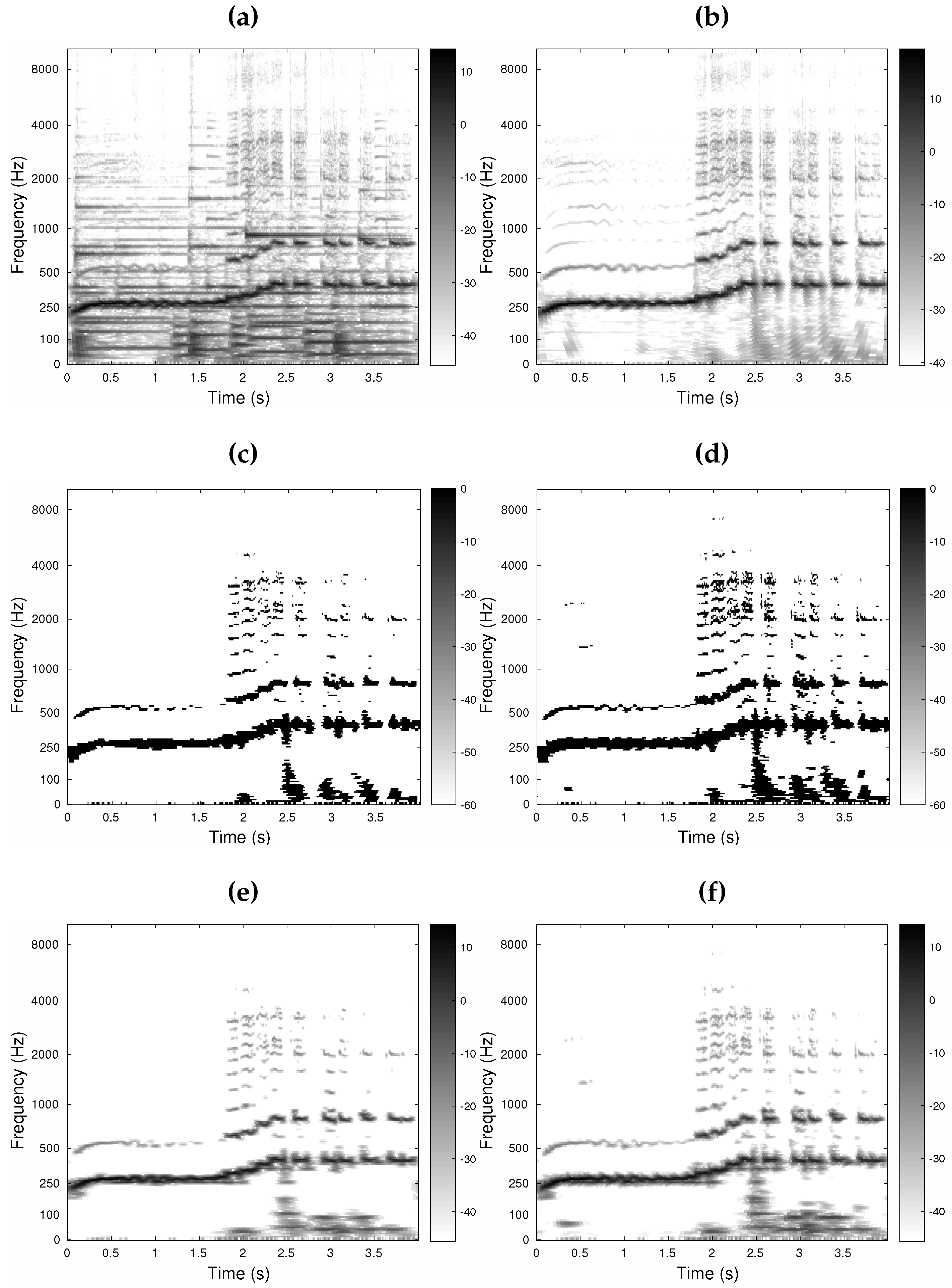
5.2. Utility for Audio Applications

5.2.1. Method

This experiment is an example application of the Audlet framework to audio source separation. Given a mixture of instrumental music and voice, we constructed various analysis–synthesis systems and separated the voice from the music. The systems were designed so as to assess the effects of perfect reconstruction, shape and bandwidth of the filter, and auditory scale on the quality of sub-channel processing at low, mid, and high redundancies. Four systems were implemented:

trev_gfb: 

a state-of-the-art gammatone FB with approximate reconstruction (the acronym trev stands for “time reversal”). The $H_k$’s followed (7) with $w(\xi )=w_{csGT,4,1.019}(\xi )$ (22) with a threshold $ϵ={10}^{-5}$. The synthesis filters $G_k(e^{2i\pi \xi })=\overline{H_k}(e^{2i\pi \xi })$. This corresponds to the baseline system used in audio applications like [11,28,29].

Audlet_gfb: 

an Audlet FB with a gammatone prototype. The $H_k$’s were computed as in trev_gfb but the synthesis stage was Algorithm 1. This system aims to compare to the baseline system and assess the effect of perfect reconstruction.

Audlet_hann: 

an Audlet FB with a Hann prototype. This system aims to assess the effect of filter shape.

STFT_hann: 

an STFT using a 1024-point Hann window. Synthesis was achieved by the dual window [2]. The time step was then adapted to match the desired redundancy $R_{\mathrm{t}}$. This corresponds to the baseline system used in most audio applications (e.g., [10,66]). This system aims to assess the use of an auditory frequency scale.

The effect of filter bandwidth was assessed by varying parameter $\beta$. Specifically, two values were tested: $\beta \in \{1,1/6\}$. Using a value of $\beta \ne 1$ means a clear departure from auditory perception but may help better resolve spectral components, particularly at high frequencies where the auditory filters become really broad (see (6)). Accordingly, many audio applications that rely on constant-Q or wavelet transforms use 12 or more bins per octave (e.g., [46,63]).

The performance of all systems were evaluated at three redundancies: $R_{\mathrm{t}}\in \{1.1,1.5,4\}$. To this end, (15) was used with $c_{bw}$ adjusted such that $R_{\mathrm{t}}$ was achieved. The quality of the separation was assessed by computing energy ratio- and perceptually-based objective measures according to [67]. Energy ratio measures include the signal-to-distortion ratio (SDR) and signal-to-artifact ratio (SAR). Perceptual measures include the overall perceptual score (OPS) and target perceptual score (TPS). OPS assesses the general audio quality of the separation, while TPS assesses the preservation of the target. All measures were computed using the PEASS toolbox [67].

The following parameters were fixed for systems trev_gfb, Audlet_gfb and Audlet_hann: $f_s$ = 22.05 kHz, $[f_{\min },f_{\max }]=[20,10,000]$, Scale = ERB, and K = 209 filters corresponding to V = 6 filters/ERB.

The signal mixture, shown in Figure 5a, was created by adding an instrumental music signal to a singing voice signal (target), shown in Figure 5b. The separation was performed by analyzing the mixture with the analysis FB, applying a binary TF mask to the sub-band components by point-wise multiplication, and computing the output signal from the modified sub-band components using the synthesis stage. This operation corresponds to the application of a frame multiplier in signal processing [9,68]. In order to create the binary masks, the target signal was analyzed by the FB and the magnitude of the coefficients was hard thresholded with a threshold of −25 dB. The threshold value was varied between −40 and −20 dB in 5-dB steps. While the threshold value did affect the separation performance, all configurations were affected equally. The value of −25 dB was selected because it yielded good separation results for both the gammatone and Hann prototypes. Four masks were created in total, one for each analysis filter’s shape and each $\beta$. The two masks for $\beta$ = 1/6 are displayed in Figure 5c,d. Because the frequency resolution of the STFT does not match those of other FBs, an additional mask was computed for the STFT.

5.2.2. Results and Discussion

Figure 5e,f show the voice signal separated using Audlet_hann and Audlet_gfb, respectively, for $R_{\mathrm{t}}$ = 4 and $\beta$ = 1/6. The objective quality measures are listed in

Table 3. Objective quality measures for the separated voice signal. The signal-to-distortion ratio (SDR) and signal-to-artifact ratio (SAR) are in dB; the larger the ratio, the better the separation result. Overall perceptual score (OPS) and target perceptual score (TPS) are without unit; they indicate scores between 0 (bad quality) and 1 (excellent quality). The corresponding audio files are available on the companion webpage. STFT: short-time Fourier transform.

System	${\mathit{R}}_{\mathbf{t}}$	SDR		SAR		OPS		TPS
		$\mathit{\beta }=$ 1	1/6	1	1/6	1	1/6	1	1/6
trev_gfb	1.1	0.1	5.8	3.2	9.2	0.26	0.26	0.06	0.12
Audlet_gfb		4.7	10.7	8.5	19.0	0.25	0.31	0.11	0.20
Audlet_hann		4.7	11.8	7.6	18.3	0.26	0.34	0.05	0.26
STFT_hann		−1.7		0.5		0.46		0.02
trev_gfb	1.5	2.4	8.5	5.7	13.5	0.24	0.30	0.11	0.17
Audlet_gfb		6.9	11.1	12.5	20.5	0.24	0.35	0.13	0.29
Audlet_hann		7.0	12.8	11.1	20.1	0.22	0.36	0.07	0.35
STFT_hann		2.4		9.2		0.22		0.04
trev_gfb	4	7.0	10.7	12.0	18.9	0.24	0.37	0.24	0.34
Audlet_gfb		9.0	11.4	18.3	21.6	0.27	0.38	0.32	0.39
Audlet_hann		11.1	13.1	19.4	21.7	0.25	0.37	0.21	0.32
STFT_hann		11.4		20.5		0.38		0.34

. Audio files are available on the companion webpage: http://www.kfs.oeaw.ac.at/audletFB. The following observations can be made.

First, system Audlet_gfb outperformed trev_gfb in most conditions. This demonstrates the role of perfect reconstruction in the quality of sub-channel processing. In other words, using the Audlet framework can improve the reconstruction quality. Note that for $\beta$ = 1/6, the performance of trev_gfb improved with increasing $R_{\mathrm{t}}$ and tended towards the performance of Audlet_gfb. This is due to the decrease in the amount of aliasing with increasing $R_{\mathrm{t}}$. For trev_gfb and $R_{\mathrm{t}}$ = 4, very little aliasing was present and a good performance was achieved despite the approximate reconstruction of trev_gfb.

Second, the performance of Audlet_hann was comparable to that of Audlet_gfb in almost every measure. Although the filter shape did not play a major role in this particular example, it may have a larger impact in other applications.

Third, for all configurations, reducing $\beta$ from 1 to 1/6 generally improved all quality measures. This suggests that, depending on the application, a departure from the human auditory perception may improve signal processing performance. In the present application, for instance, finely tuned filters are required to resolve all harmonics and therefore properly separate the signals.

Finally, while STFT_hann performed comparably to Audlet_hann at the highest R, the performance of STFT_hann dropped at mid and low redundancies. This suggests that using an auditory frequency scale may improve signal processing performance at low redundancies.

6. Conclusions

A framework for the construction of oversampled perfect-reconstruction FBs with filters distributed on auditory frequency scales has been presented. This framework was motivated by auditory perception and targeted at audio signal processing; it has thus been named “Audlet”. The proposed approach has its foundation in the mathematical theory of frames. The analysis FB design is directly performed in the frequency domain and allows for various filter shapes, and uniform or non-uniform settings with low redundancies. The synthesis is achieved using a (heuristic) preconditioned conjugate-gradient iterative algorithm. The convergence of the algorithm has been observed for Audlet FBs that constitute a frame. This is possible even for redundancies close to 1. For higher redundancies and filters with a compact support in the frequency domain, a so-called “painless” system can be achieved. In this case the exact dual FB can be calculated, which in turn results in a computationally more efficient synthesis.

We showed how to construct a gammatone FB with perfect reconstruction. The proposed gammatone FB was compared to widely used state-of-the-art implementations of gammatone FB with approximate reconstruction. The results showed the better performance of the proposed approach in terms of reconstruction error and stability, especially at low redundancies. An example application of the framework to the task of audio source separation demonstrated its utility for audio processing.

Overall, the Audlet framework provides a versatile and efficient FB design that is highly suitable for audio applications requiring stability, perfect reconstruction, and a flexible choice of redundancy. The framework is implemented in the free Matlab/Octave toolbox LTFAT [61,62].

References

1. Flandrin, P. Time-Frequency/Time-Scale Analysis; Wavelet Analysis and Its Application; Academic Press: San Diego, CA, USA, 1999; Volume 10. [Google Scholar]
2. Gröchenig, K. Foundations of Time-Frequency Analysis; Birkhäuser: Boston, MA, USA, 2001. [Google Scholar]
3. Kamath, S.; Loizou, P. A multi-band spectral subtraction method for enhancing speech corrupted by colored noise. In Proceedings of the 2002 IEEE International Conference on Acoustics, Speech, and Signal Processing, Orlando, FL, USA, 13–17 May 2002; Volume 4. [Google Scholar]
4. Majdak, P.; Balazs, P.; Kreuzer, W.; Dörfler, M. A time-frequency method for increasing the signal-to-noise ratio in system identification with exponential sweeps. In Proceedings of the 2011 IEEE International Conference on Acoustics, Speech and Signal Processing (ICASSP), Prague, Czech Republic, 22–27 May 2011. [Google Scholar]
5. International Organization for Standardization. ISO/IEC 11172-3: Information Technology—Coding of Moving Pictures and Associated Audio for Digital Storage Media at up to About 1.5 Mbits/s, Part 3: Audio; Technical Report; International Organization for Standardization (ISO): Geneva, Switzerland, 1993. [Google Scholar]
6. International Organization for Standardization. ISO/IEC 13818-7: 13818-7: Generic Coding of Moving Pictures and Associated Audio: Advanced Audio Coding; Technical Report; International Organization for Standardization (ISO): Geneva, Switzerland, 1997. [Google Scholar]
7. International Organization for Standardization. ISO/IEC 14496-3/AMD-2: Information Technology—Coding of Audio-Visual Objects, Amendment 2: New Audio Profiles; Technical Report; International Organization for Standardization (ISO): Geneva, Switzerland, 2006. [Google Scholar]
8. Průša, Z.; Holighaus, N. Phase vocoder done right. In Proceedings of the 25th European Signal Processing Conference (EUSIPCO–2017), Kos Island, Greece, 28 August–2 September 2017; pp. 1006–1010. [Google Scholar]
9. Sirdey, A.; Derrien, O.; Kronland-Martinet, R. Adjusting the spectral envelope evolution of transposed sounds with gabor mask prototypes. In Proceedings of the 13th International Conference on Digital Audio Effects (DAFx-10), Graz, Austria, 10 September 2010; pp. 1–7. [Google Scholar]
10. Leglaive, S.; Badeau, R.; Richard, G. Multichannel Audio Source Separation with Probabilistic Reverberation Priors. IEEE/ACM Trans. Audio Speech Lang. Process. 2016, 24, 2453–2465. [Google Scholar] [CrossRef]
11. Gao, B.; Woo, W.L.; Khor, L.C. Cochleagram-based audio pattern separation using two-dimensional non-negative matrix factorization with automatic sparsity adaptation. J. Acoust. Soc. Am. 2014, 135, 1171–1185. [Google Scholar]
12. Unoki, M.; Akagi, M. A method of signal extraction from noisy signal based on auditory scene analysis. Speech Commun. 1999, 27, 261–279. [Google Scholar] [CrossRef]
13. Bertin, N.; Badeau, R.; Vincent, E. Enforcing Harmonicity and Smoothness in Bayesian Non-Negative Matrix Factorization Applied to Polyphonic Music Transcription. IEEE Trans. Audio Speech Lang. Process. 2010, 18, 538–549. [Google Scholar] [CrossRef]
14. Cvetković, Z.; Johnston, J.D. Nonuniform oversampled filter banks for audio signal processing. IEEE Speech Audio Process. 2003, 11, 393–399. [Google Scholar] [CrossRef]
15. Smith, J.O. Spectral Audio Signal Processing. Online Book. 2011. Available online: http://ccrma.stanford.edu/~jos/sasp/ (accessed on 9 January 2018).
16. Akkarakaran, S.; Vaidyanathan, P. Nonuniform filter banks: New results and open problems. In Beyond Wavelets; Studies in Computational Mathematics; Elsevier: Amsterdam, The Netherlands, 2003; Volume 10, pp. 259–301. [Google Scholar]
17. Vaidyanathan, P. Multirate Systems And Filter Banks; Electrical Engineering, Electronic and Digital Design; Prentice Hall: Englewood Cliffs, NJ, USA, 1993. [Google Scholar]
18. Vetterli, M.; Kovačević, J. Wavelets and Subband Coding; Prentice Hall PTR: Englewood Cliffs, NJ, USA, 1995. [Google Scholar]
19. Kovačević, J.; Vetterli, M. Perfect reconstruction filter banks with rational sampling factors. IEEE Trans. Signal Process. 1993, 41, 2047–2066. [Google Scholar]
20. Balazs, P.; Holighaus, N.; Necciari, T.; Stoeva, D. Frame theory for signal processing in psychoacoustics. In Excursions in Harmonic Analysis; Applied and Numerical Harmonic Analysis; Birkäuser: Basel, Switzerland, 2017; Volume 5, pp. 225–268. [Google Scholar]
21. Bölcskei, H.; Hlawatsch, F.; Feichtinger, H. Frame-theoretic analysis of oversampled filter banks. IEEE Trans. Signal Process. 1998, 46, 3256–3268. [Google Scholar] [CrossRef]
22. Cvetković, Z.; Vetterli, M. Oversampled filter banks. IEEE Trans. Signal Process. 1998, 46, 1245–1255. [Google Scholar] [CrossRef]
23. Strohmer, T. Numerical algorithms for discrete Gabor expansions. In Gabor Analysis and Algorithms: Theory and Applications; Feichtinger, H.G., Strohmer, T., Eds.; Birkhäuser: Boston, MA, USA, 1998; pp. 267–294. [Google Scholar]
24. Härmä, A.; Karjalainen, M.; Savioja, L.; Välimäki, V.; Laine, U.K.; Huopaniemi, J. Frequency-Warped Signal Processing for Audio Applications. J. Audio Eng. Soc. 2000, 48, 1011–1031. [Google Scholar]
25. Gunawan, T.S.; Ambikairajah, E.; Epps, J. Perceptual speech enhancement exploiting temporal masking properties of human auditory system. Speech Commun. 2010, 52, 381–393. [Google Scholar] [CrossRef]
26. Balazs, P.; Laback, B.; Eckel, G.; Deutsch, W.A. Time-Frequency Sparsity by Removing Perceptually Irrelevant Components Using a Simple Model of Simultaneous Masking. IEEE Trans. Audio Speech Lang. Process. 2010, 18, 34–49. [Google Scholar] [CrossRef]
27. Chardon, G.; Necciari, T.; Balazs, P. Perceptual matching pursuit with Gabor dictionaries and time-frequency masking. In Proceedings of the 39th International Conference on Acoustics, Speech, and Signal Processing (ICASSP 2014), Florence, Italy, 4–9 May 2014. [Google Scholar]
28. Wang, D.; Brown, G.J. Computational Auditory Scene Analysis: Principles, Algorithms, and Applications; Wiley-IEEE Press: Hoboken, NJ, USA, 2006. [Google Scholar]
29. Li, P.; Guan, Y.; Xu, B.; Liu, W. Monaural Speech Separation Based on Computational Auditory Scene Analysis and Objective Quality Assessment of Speech. IEEE Trans. Audio Speech Lang. Process. 2006, 14, 2014–2023. [Google Scholar] [CrossRef]
30. Glasberg, B.R.; Moore, B.C.J. Derivation of auditory filter shapes from notched-noise data. Hear. Res. 1990, 47, 103–138. [Google Scholar] [CrossRef]
31. Rosen, S.; Baker, R.J. Characterising auditory filter nonlinearity. Hear. Res. 1994, 73, 231–243. [Google Scholar] [CrossRef]
32. Lyon, R. All-pole models of auditory filtering. Divers. Audit. Mech. 1997, 205–211. [Google Scholar]
33. Irino, T.; Patterson, R.D. A Dynamic Compressive Gammachirp Auditory Filterbank. Audio Speech Lang. Process. 2006, 14, 2222–2232. [Google Scholar] [CrossRef] [PubMed]
34. Verhulst, S.; Dau, T.; Shera, C.A. Nonlinear time-domain cochlear model for transient stimulation and human otoacoustic emission. J. Acoust. Soc. Am. 2012, 132, 3842–3848. [Google Scholar] [CrossRef] [PubMed]
35. Feldbauer, C.; Kubin, G.; Kleijn, W.B. Anthropomorphic coding of speech and audio: A model inversion approach. EURASIP J. Adv. Signal Process. 2005, 2005, 1334–1349. [Google Scholar] [CrossRef]
36. Decorsière, R.; Søndergaard, P.L.; MacDonald, E.N.; Dau, T. Inversion of Auditory Spectrograms, Traditional Spectrograms, and Other Envelope Representations. IEEE Trans. Audio Speech Lang. Process. 2015, 23, 46–56. [Google Scholar] [CrossRef]
37. Lyon, R.; Katsiamis, A.; Drakakis, E. History and future of auditory filter models. In Proceedings of the 2010 IEEE International Symposium on Circuits and Systems (ISCAS), Paris, France, 30 May–2 June 2010; pp. 3809–3812. [Google Scholar]
38. Patterson, R.D.; Robinson, K.; Holdsworth, J.; McKeown, D.; Zhang, C.; Allerhand, M.H. Complex sounds and auditory images. In Proceedings of the Auditory Physiology and Perception: 9th International Symposium on Hearing, Carcens, France, 9–14 June 1991; pp. 429–446. [Google Scholar]
39. Hohmann, V. Frequency analysis and synthesis using a Gammatone filterbank. Acta Acust. United Acust. 2002, 88, 433–442. [Google Scholar]
40. Lin, L.; Holmes, W.; Ambikairajah, E. Auditory filter bank inversion. In Proceedings of the 2001 IEEE International Symposium on Circuits and Systems (ISCAS 2001), Sydney, Australia, 6–9 May 2001; Volume 2, pp. 537–540. [Google Scholar]
41. Slaney, M. An Efficient Implementation of the Patterson-Holdsworth Auditory Filter Bank; Apple Computer Technical Report No. 35; Apple Computer, Inc.: Cupertino, CA, USA; 1993; pp. 1–42. [Google Scholar]
42. Holdsworth, J.; Nimmo-Smith, I.; Patterson, R.D.; Rice, P. Implementing a Gammatone Filter Bank; Annex c of the Svos Final Report (Part A: The Auditory Filterbank); MRC Applied Psychology Unit: Cambridge, UK, 1988. [Google Scholar]
43. Darling, A. Properties and Implementation of the Gammatone Filter: A Tutorial; Technical Report; University College London, Department of Phonetics and Linguistics: London, UK, 1991; pp. 43–61. [Google Scholar]
44. Strahl, S.; Mertins, A. Analysis and design of gammatone signal models. J. Acoust. Soc. Am. 2009, 126, 2379–2389. [Google Scholar] [PubMed]
45. Balazs, P.; Dörfler, M.; Holighaus, N.; Jaillet, F.; Velasco, G. Theory, Implementation and Applications of Nonstationary Gabor Frames. J. Comput. Appl. Math. 2011, 236, 1481–1496. [Google Scholar] [CrossRef] [PubMed]
46. Holighaus, N.; Dörfler, M.; Velasco, G.; Grill, T. A framework for invertible, real-time constant-Q transforms. Audio Speech Lang. Process. 2013, 21, 775–785. [Google Scholar] [CrossRef]
47. Holighaus, N.; Wiesmeyr, C.; Průša, Z. A class of warped filter bank frames tailored to non-linear frequency scales. arXiv, 2016; arXiv:1409.7203. [Google Scholar]
48. Necciari, T.; Balazs, P.; Holighaus, N.; Søndergaard, P. The ERBlet transform: An auditory-based time-frequency representation with perfect reconstruction. In Proceedings of the 2013 IEEE International Conference on Acoustics, Speech and Signal Processing (ICASSP), Vancouver, BC, Canada, 26–31 May 2013; pp. 498–502. [Google Scholar]
49. Trefethen, L.N.; Bau, D., III. Numerical Linear Algebra; SIAM: Philadelphia, PA, USA, 1997. [Google Scholar]
50. Moore, B.C.J. An Introduction to the Psychology of Hearing, 6th ed.; Emerald Group Publishing: Bingley, UK, 2012. [Google Scholar]
51. Zwicker, E.; Terhardt, E. Analytical expressions for critical-band rate and critical bandwidth as a function of frequency. J. Acoust. Soc. Am. 1980, 68, 1523–1525. [Google Scholar] [CrossRef]
52. O’shaughnessy, D. Speech Communication: Human and Machine; Addison-Wesley: Boston, MA, USA, 1987. [Google Scholar]
53. Daubechies, I.; Grossmann, A.; Meyer, Y. Painless nonorthogonal expansions. J. Math. Phys. 1986, 27, 1271–1283. [Google Scholar] [CrossRef]
54. Průša, Z.; Søndergaard, P.L.; Rajmic, P. Discrete Wavelet Transforms in the Large Time-Frequency Analysis Toolbox for Matlab/GNU Octave. ACM Trans. Math. Softw. 2016, 42, 32:1–32:23. [Google Scholar] [CrossRef]
55. Hestenes, M.R.; Stiefel, E. Methods of conjugate gradients for solving linear systems. J. NBS 1952, 49, 409–436. [Google Scholar] [CrossRef]
56. Gröchenig, K. Acceleration of the frame algorithm. IEEE Trans. Signal Process. 1993, 41, 3331–3340. [Google Scholar] [CrossRef]
57. Eisenstat, S.C. Efficient implementation of a class of preconditioned conjugate gradient methods. SIAM J. Sci. Stat. Comput. 1981, 2, 1–4. [Google Scholar] [CrossRef]
58. Balazs, P.; Feichtinger, H.G.; Hampejs, M.; Kracher, G. Double preconditioning for Gabor frames. IEEE Trans. Signal Process. 2006, 54, 4597–4610. [Google Scholar] [CrossRef]
59. Christensen, O. An Introduction to Frames and Riesz Bases; Applied and Numerical Harmonic Analysis; Birkhäuser: Boston, MA, USA, 2016. [Google Scholar]
60. Smith, J.O. Audio FFT filter banks. In Proceedings of the 12th International Conference on Digital Audio Effects (DAFx-09), Como, Italy, 1–4 September 2009; pp. 1–8. [Google Scholar]
61. Søndergaard, P.L.; Torrésani, B.; Balazs, P. The Linear Time Frequency Analysis Toolbox. Int. J. Wavelets Multiresolut. Inf. Process. 2012, 10, 1250032. [Google Scholar] [CrossRef]
62. Průša, Z.; Søndergaard, P.L.; Holighaus, N.; Wiesmeyr, C.; Balazs, P. The large time-frequency analysis toolbox 2.0. In Sound, Music, and Motion; Springer: Berlin, Germany, 2014; pp. 419–442. [Google Scholar]
63. Schörkhuber, C.; Klapuri, A.; Holighaus, N.; Dörfler, M. A matlab toolbox for efficient perfect reconstruction time-frequency transforms with log-frequency resolution. In Proceedings of the Audio Engineering Society 53rd International Conference on Semantic Audio, London, UK, 27–29 January 2014. [Google Scholar]
64. Velasco, G.A.; Holighaus, N.; Dörfler, M.; Grill, T. Constructing an invertible constant-Q transform with nonstationary Gabor frames. In Proceedings of the 14th International Conference on Digital Audio Effects (DAFx-11), Paris, France, 19–23 September 2011; pp. 93–99. [Google Scholar]
65. Lehoucq, R.; Sorensen, D.C. Deflation Techniques for an Implicitly Re-Started Arnoldi Iteration. SIAM J. Matrix Anal. Appl. 1996, 17, 789–821. [Google Scholar] [CrossRef]
66. Le Roux, J.; Vincent, E. Consistent Wiener Filtering for Audio Source Separation. Signal Process. Lett. IEEE 2013, 20, 217–220. [Google Scholar] [CrossRef] [Green Version]
67. Emiya, V.; Vincent, E.; Harlander, N.; Hohmann, V. Subjective and Objective Quality Assessment of Audio Source Separation. IEEE Trans. Audio Speech Lang. Process. 2011, 19, 2046–2057. [Google Scholar] [CrossRef] [Green Version]
68. Balazs, P. Basic Definition and Properties of Bessel Multipliers. J. Math. Anal. Appl. 2007, 325, 571–585. [Google Scholar] [CrossRef]
Figure 1. General structure of a non-uniform analysis filter bank (FB) ( H k , d k ) k with H k being the z-transform of the impulse response h k [ n ] of the filter, also denoted as A ( · , ( H k , d k ) k ) .
Applsci 08 00096 g001
Figure 2. General structure of a non-uniform synthesis FB ( G k , d k ) k , also denoted by S ˜ ( · , ( G k , d k ) k ) .
Applsci 08 00096 g002
Figure 3. General structure of a synthesis system. S is a linear operator that maps the sub-band components y k to an output signal x ˜ .
Applsci 08 00096 g003
Figure 4. Illustration of the frequency allocations of the filters H 0 (red line) and H K (green line) given the restricted frequency response H 0 ( r ) ( ξ ) (dashed line) of an FB.
Applsci 08 00096 g004
Figure 5. Source separation for R t = 4 and β = 1/6 displayed as time-frequency (TF) plots: the magnitude of each sub-band component (in dB) as a function of time (in s). (a) Shows the mixture analyzed by a gammatone FB; (b) Shows the target (voice) analyzed by a gammatone FB; (c) Shows the binary mask obtained for Audlet_hann; (d) Shows the binary mask obtained for trev_gfb and Audlet_gfb—the black and white dots in the masks represent ‘1’ and ‘0’ entries, respectively; (e,f) Show the target separated by Audlet_hann and Audlet_gfb, respectively.
Applsci 08 00096 g005