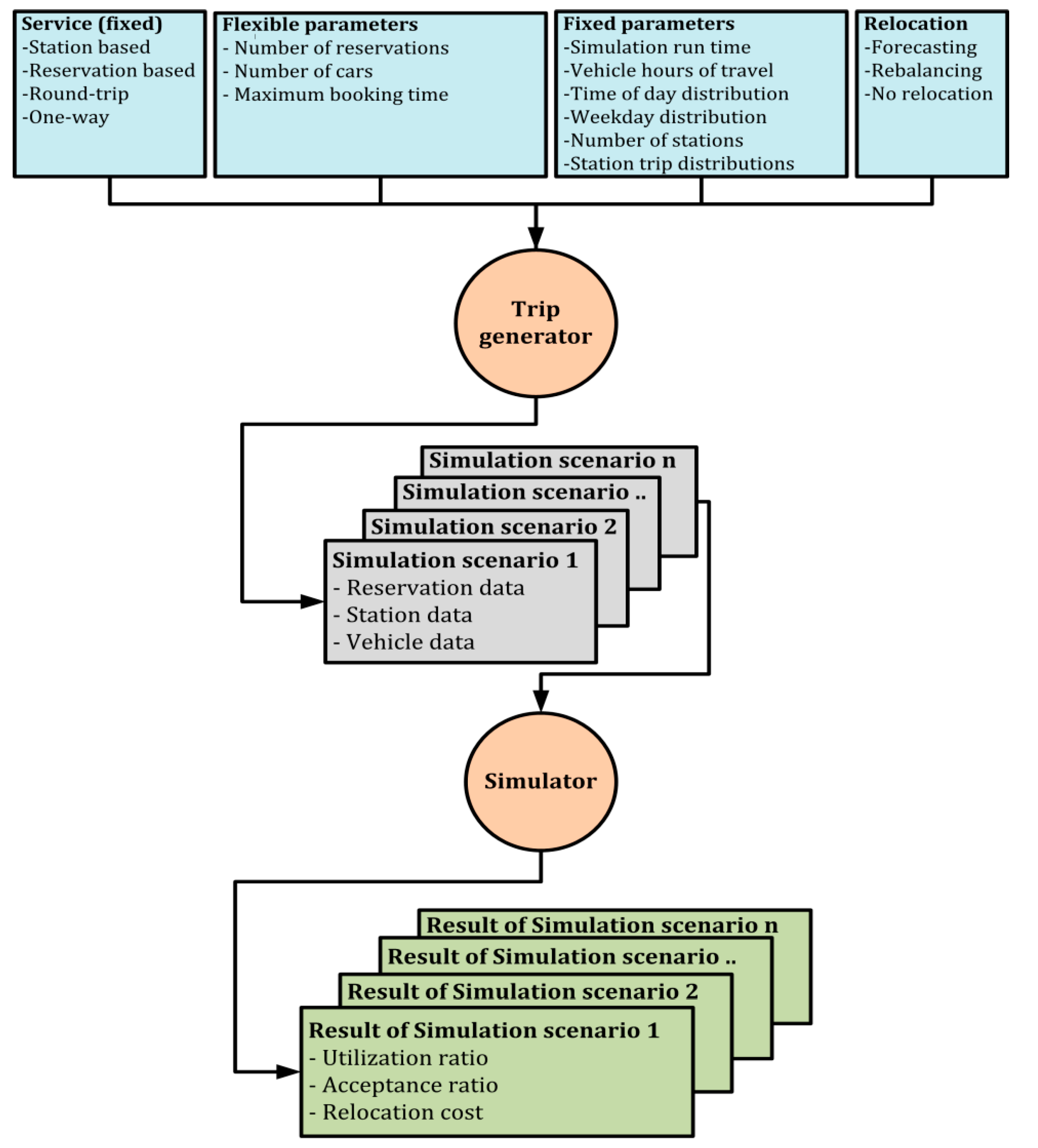
3.1. Carsharing Simulation
This paper used a simulation model for a station based one-way service, which allowed customers to use a car and return it to a different station. Reservation based carsharing was applied, i.e., all the customers were required to reserve a vehicle in advance. Round-trip and one-way services were considered, and if a company operated a one-way service, it also allowed customers to use the round-trip service since the round-trip service is a standard service for car sharing businesses. The proportion of round-trip and one-way reservations was assumed to be 50:50, i.e., one-way reservations comprised 50% of the total reservations with the remainder being round-trip reservations. The simulation was run for every reasonable combination of parameters (flexible parameters), such as the number of cars, number of reservations, and maximum booking time. Customer travel demand of the carsharing company (fixed parameters) was used as a simulation input, such as vehicle hour trips (VHT), time of day, day of the week, number of stations, and trip distribution of the stations. Forecasting and rebalancing relocation models were compared for each simulation scenario, as shown in
Figure 1.
First, simulation scenarios containing artificial data (reservation, station, and vehicle data) were generated by the trip generator, based on customer travel demand, the relocation model, number of vehicles, and reservations. Different combinations of parameters generated different simulation scenarios.
Second, the simulator evaluated every scenario, i.e., the combination of travel demands with the number of cars, number of reservations, and the relocation model. For each scenario, the generated artificial data was updated once the simulation process was completed. The simulation checks customer reservations, so some reservation, station, and vehicle data changed during the simulation process.
Finally, the simulation results were presented and analyzed to define the performance of the relocation model in one-way car sharing. Output parameters included the utilization ratio, acceptance ratio, and relocation cost. The simulation implemented DES, generating a list of events from the reservation based one-way system, such as calling, assign, starting, and ending times. A reservation via phone/internet (calling time) is required. Once the reservation is accepted, the system assigns a parked car to a particular reservation. Customers visit the departure station at the starting time to pick up the booked car and return it to the destination station at the ending time.
In this study, last-minute reservation based one-way carsharing system with 10 stations will be evaluated by the simulation model. The reservation system allows customers to request a reservation with a maximum of three hours before the starting time. To guarantee the vehicle availability to the customer, we used a strict policy for reservation, i.e., the car is reserved until it is picked-up by the customer. Previous research (Boyaci et al. [
18]) used dynamic relocation (relocate during the day) and safety gap (i.e., 30 min of additional time, starting at the end time reservation to guarantee the space at the destination station; and avoid the car being reserved and relocated until the end of the safety gap duration) [
18]. In our study, static relocation is used as we only focus on the performance of the forecasting relocation model at the end of the day. Different operational policies were applied in our study, such as when the customer made the reservation, a space at the destination station was reserved by the system starting from the reservation time until the end of the simulation time. It will prevent other customers from parking their car until the status of the particular space is changed to free again (i.e., the car is out from the station). In addition, we assumed that every customer returned the car at the returning time precisely, thus the next reservation is ready to be made.
The simulation allowed round-trip and one-way service: the round-trip destination station was the same as the departure station, whereas the one-way destination station differed from the departure station.
3.2. Data Collection
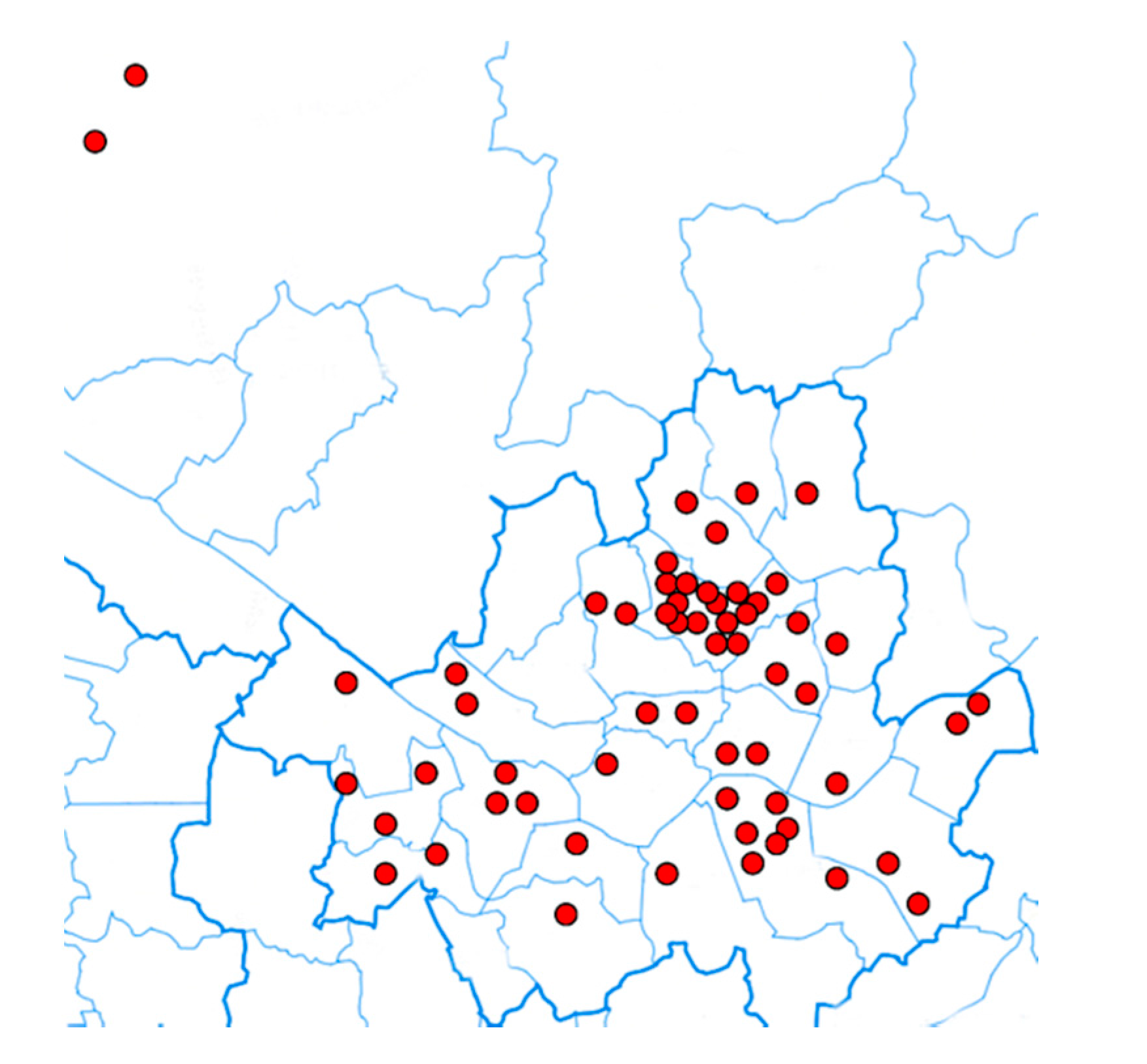
This paper used a real carsharing service dataset from Korea, provided by HanCar (carsharing company in Korea), which operates in Seoul Metropolitan City. The customer reservation data was gathered for three months from May to July 2015. HanCar operates a reservation based round-trip service with 59 stations and 103 vehicles spread around the Seoul area.
Figure 2 shows the carsharing station locations as red markers.
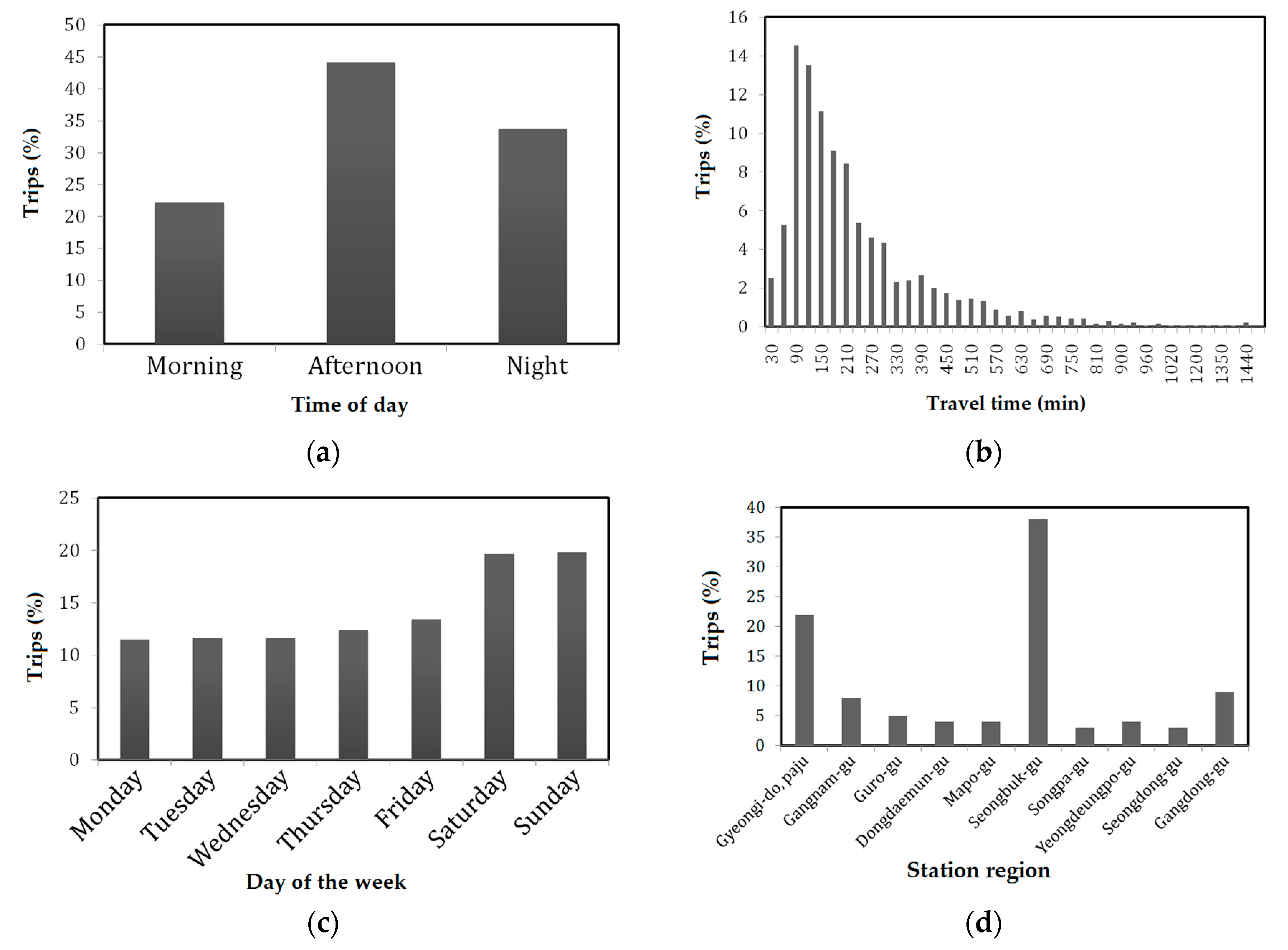
The simulation input follows the time of day travel pattern, where customer reservation proportions for morning, afternoon, and evening were 22.15%, 44.15%, and 33.70%, respectively, as shown in
Figure 3a. The HanCar dataset showed that the average customer VHT was 120 min, with 30 min as the minimum and the maximum as one day (
Figure 3b). However, in order to simplify our simulation input (but still follow the HanCar distribution), the trip duration is assigned for 2, 4, and 6 h and its distributions are 20%, 50%, and 30%, respectively. The percentage of trips was lowest at the beginning of the week, increasing as the week progressed, as shown in
Figure 3c.
The original 59 stations are grouped into 10 stations based on the district area (administrative unit). In
Figure 2, the original stations and district boundaries are presented in red and blue colors respectively. In our dataset, the original stations mostly have three cars and their customer demands are almost similar. By grouping the original stations based on the district, it will create high unbalance demand since some of districts have more stations compared to others. It is expected that cars become unbalanced, with most cars ending up in unpopular departure groups, and most customers (from the high demand group) are unable to make a reservation. In this situation, the forecasting relocation can be evaluated in terms of its capability to solve the high unbalance demand problem. To simplify the simulation process, only the top 10 highest groups are used as inputs of the simulation. Based on the departure distribution of each group, customers mostly departed from Seongbuk-gu and Gyeongido-paju (38% and 22%, respectively), and the detailed departure distribution is shown in
Figure 3d. However, the clustering based on the district is not the only solution, as other studies (Boyaci et al. [
18]) used different techniques to group the stations. The k-medoid based algorithm was used to cluster the stations.
The HanCar company only offered round-trip service (i.e., the same destination and departure station), whereas the simulation also considered one-way service. Boyaci et al. have proposed the scenario to convert the round-trip data into one-way data [
28]. Given the GPS data, the conversion is done by splitting the single round-trip data into multiple one-way data when the idle time of the rented vehicle at a given location exceeded one hour. However, due to the limitation of the dataset (i.e., GPS data), other types of conversion were applied. To generate the artificial reservation data for different departure and destination stations, the trip generator considered that the departure station followed the HanCar distribution and the destination station was assigned randomly.
3.3. Evaluation Criteria
Three evaluation criteria were defined in the simulation to evaluate the relocation model performances: car utilization ratio, reservation acceptance ratio, and relocation cost.
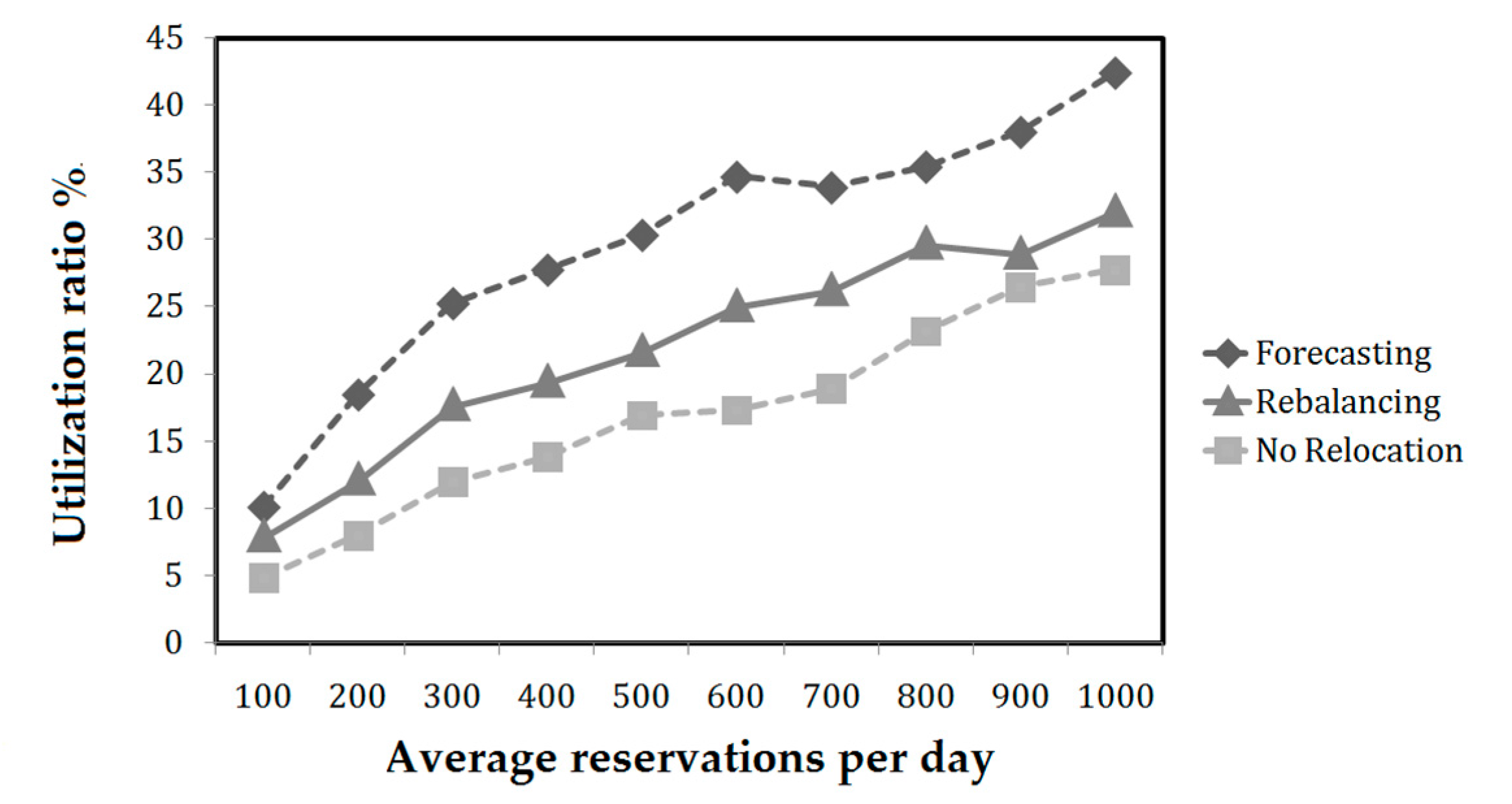
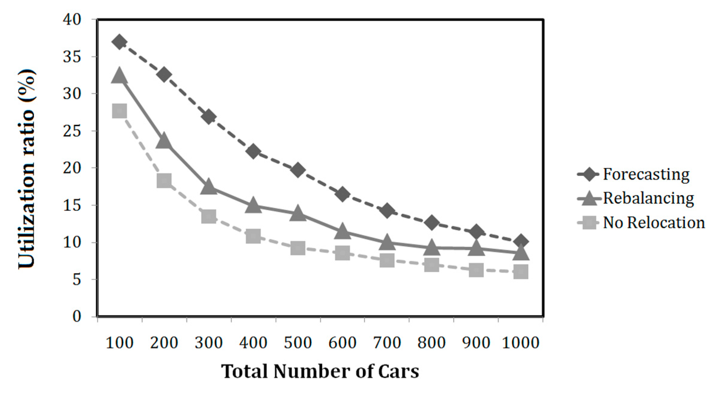
The car utilization ratio is the percentage of total actual driving hours of rented cars over total possible driving hours of cars,
Alfian et al. has revealed that the utilization ratio is proportional to the average profit per day [
27]. Thus, it is important that the carsharing company needs to ensure that all cars can be rented (fully operated) to increase profit.
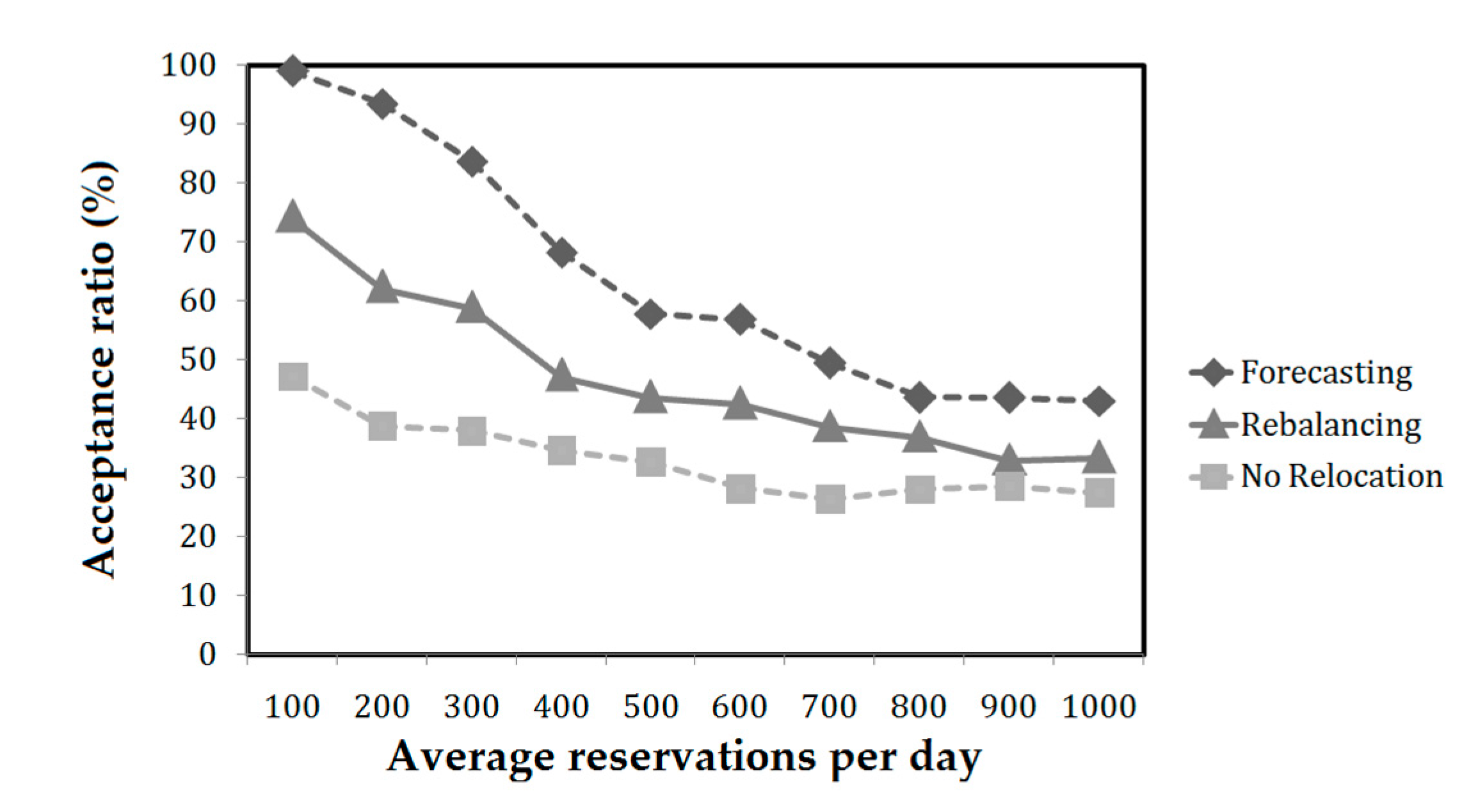
The acceptance ratio is the number of reservations that have been accepted compared to the total number of requested reservations,
An accepted reservation means that when a customer makes a reservation, the carsharing reservation system checks whether there is an available car at the departure station and free parking space at the destination station. In this study, we assumed that there were no cancelations for an earlier reservation, and that the customer drives the car from the departure station at the starting time and parks the car at the expected destination at the ending time of the reservation. Thus, the acceptance ratio probes customer satisfaction.
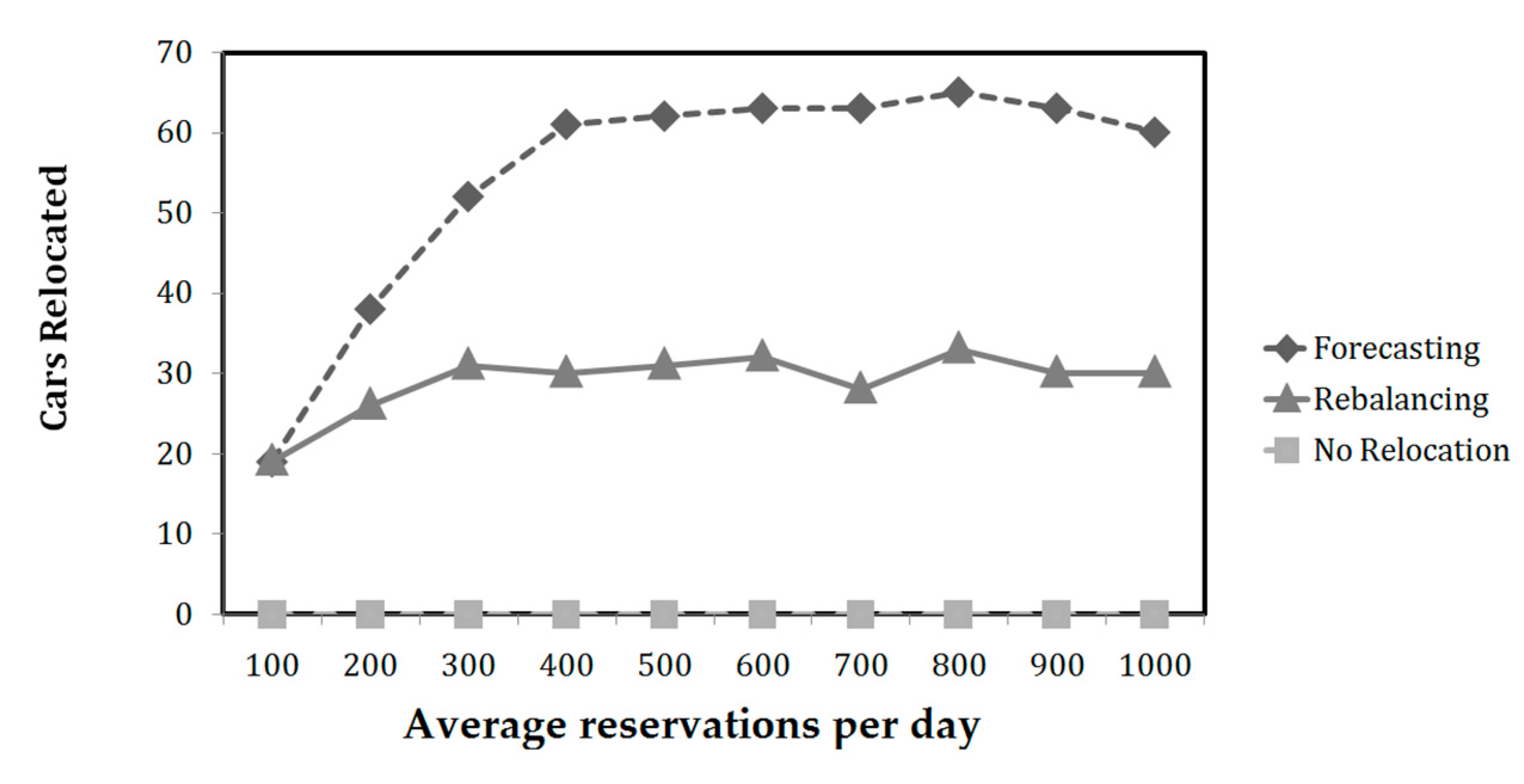
Relocation cost provides information about the number of cars being relocated by the operator at the end of the day,
Carsharing companies normally want to reduce the relocation cost, and, hence, increase the total profit. The relocation will be triggered at the end of the day (midnight). The stations are located in the downtown area which are close to each other and the maximum relocation time from one station to another is no more than 1 h. Thus in this study, a 1 h relocation time was assumed at midnight, when cars would generally not be operated due to sparse reservations. The status of a relocated car should be a parked car, i.e., there was no existing reservation for the car.
3.4. Forecasting Relocation Model
This paper used forecasting relocation to solve the imbalanced distribution of cars at each station. Thus, the performance of the forecasting model, multilayer perceptron (MLP), must be evaluated first. The MLP consisted of input, hidden, and output layers. Inputs were fed forward from the input layer through the hidden layer(s), ultimately providing the output. For an untrained network, the output differs from the known targets. The training process consisted of estimating weights to minimize deviations between the network outputs and actual data. The deviations were then propagated backwards through the network and weights were adjusted to reduce error. Detailed explanations of MLP are described elsewhere, e.g., [
29].
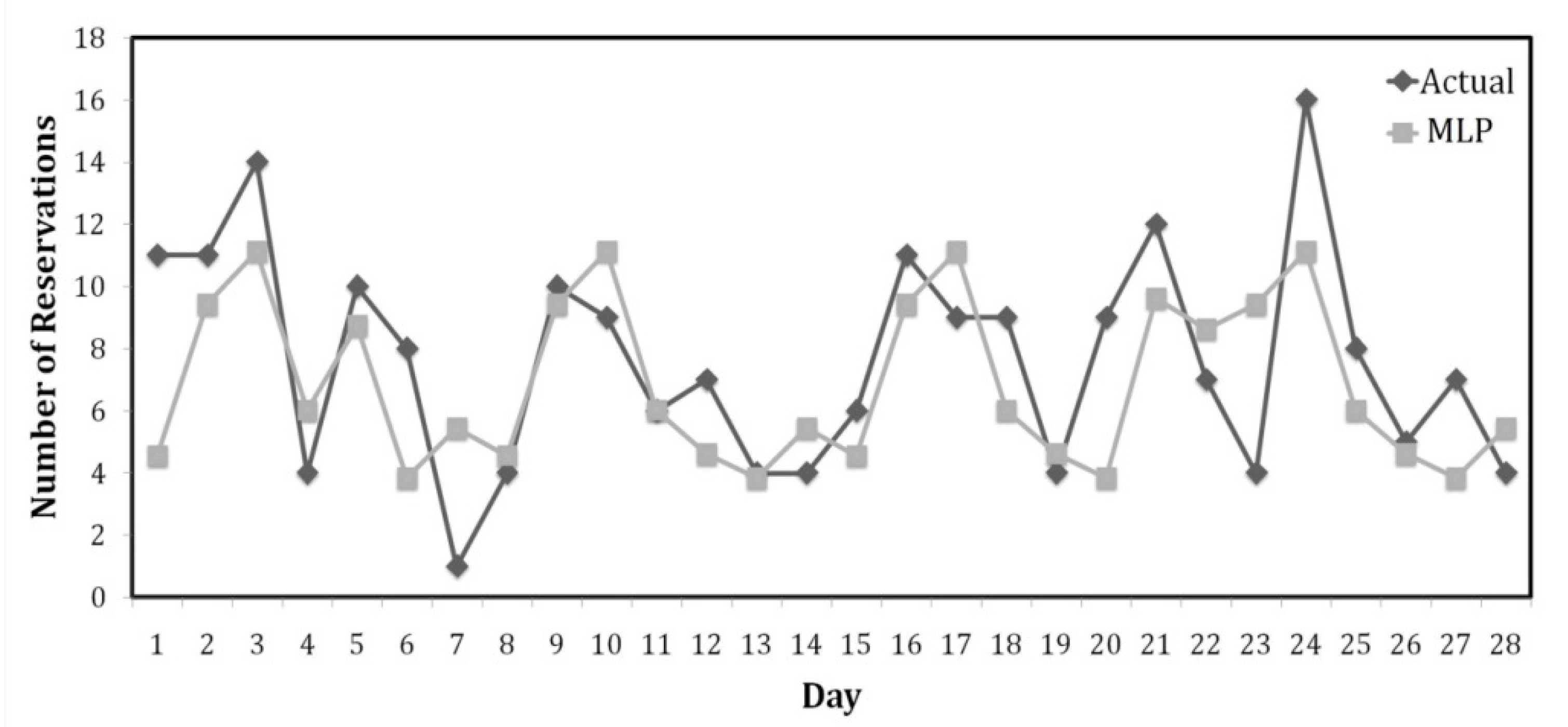
MLP was used to predict the daily number of trips for each station, which allows prediction of the number of cars needed at each station. In our study, the daily demand is considered as an input to be used by MLP for prediction. The demand based on the time (i.e., different demand between morning, afternoon, and night) is not considered in this study as we only focus on the static relocation (relocation is done at the end of the day). Thus, predicting the total number of cars needed by each station for the next day and relocating the cars at midnight are the main tasks in order to maximize the customer demand. The MLP was trained for a particular month using data from the previous 3 months, where the oldest 2 months comprised the training set and the most recent month comprised the validation set (28 days). For a particular station, the output layer was the daily total trips made by customers to particular stations and the input layer included the day type and number of trips in the previous week. Day types are defined by eight binary digits: Monday, Tuesday, Wednesday, Thursday, Friday, Saturday, or Sunday, and holiday, where 0 was “no” and 1 was “yes”. The number of trips in the previous week was the total reservations by customers in the previous week for that particular station. The training and testing process was implemented in the Weka 3.6 data mining tool (University of Waikato, Hamilton, New Zealand).
Figure 4 shows the trip predictions for 28 days in the Seongbuk-gu area.
MLP captured the daily number of reservation patterns for 28 days in Seongbuk-gu area quite well. The mean absolute error and root mean squared error of the forecasting model were 2.9003 and 3.5166 trips, respectively. Daily reservation forecasting was also applied to the other stations (details not shown), and overall the MLP model predicted the daily reservations made by the customer in each station accurately, i.e., with low errors.
The relocation model proposed in this study was based on periodical relocation, i.e., relocation was triggered at the end of the day (midnight), with the total number of cars required at each station for the next day predicted by the forecasting model. That is, this relocation was not triggered by customer demand (as per dynamic relocation). Consequently, the total number of relocations is expected to be lower than dynamic relocation, i.e., lower relocation cost.
Predicting the total number of cars based on customer reservation demands is also expected to increase the system utilization. To implement vehicle relocations, the operator sets the vehicle inventory threshold at each station. The vehicle inventory threshold is defined as present cars (number of present or parked cars)—predicted cars (number of predicted cars for the next day). The predicted cars are calculated based on the predicted customer demand (trips) using the MLP model, thus the high demand stations will have a high number of predicted cars. The system relocates the number of cars from an overstocked station (exceeding the inventory threshold) to the nearest understocked station (below the threshold) in terms of the lowest travel cost at the time of relocation.
3.5. Simulation Input and Experimental Scenario
The trip generator generates three matrices from the data distributions: reservation data, vehicle data, and station data. Customer reservation data is presented as
, where
m is the total number of reservations, and
n is the total hours of simulation, e.g.,
where
= {
calling, 0, 6, 9, 4, 7, 0} represents {
RESERVATION_EVENT,
DECISION,
DEPARTURE_STATION_ID,
DESTINATION_STATION_ID,
STARTING_TIME, ENDING_TIME,
VEHICLE_ID}, respectively. Thus, the above case means that the customer made a reservation (calling) to the system to request a car from station id 6 at the 4th hour to station id 9 at the 7th hour. In our study, the full hour reservation made by customers is assumed. The default
DECISION is always initialized to 0.
Station data is presented as
, where
q is the number of stations, and
n is the number of hours for the simulation, e.g.,
where
=
represents {
STATION_ID,
TOTAL_LOTS,
VIN,
VOUT,
VPRESENT,
AV_SPACE}, respectively. Thus, this entry means that initially station ID 1 has 25 lots, there is no car expected to come in (VIN) or go out (VOUT) from this particular station, the total of parked cars (VPRESENT) is 10, and the available space (AV_SPACE) is 15.
Finally, the vehicle data is presented as
, where
p is the number of vehicles, and
n is the number of hours for the simulation, e.g.,
where
=
represents {
VEHICLE_ID,
VEHICLE_STATUS,
CURRENT_STATION}, respectively. Thus, this entry means that at the initial time vehicle id 1 was parked at station ID 1.
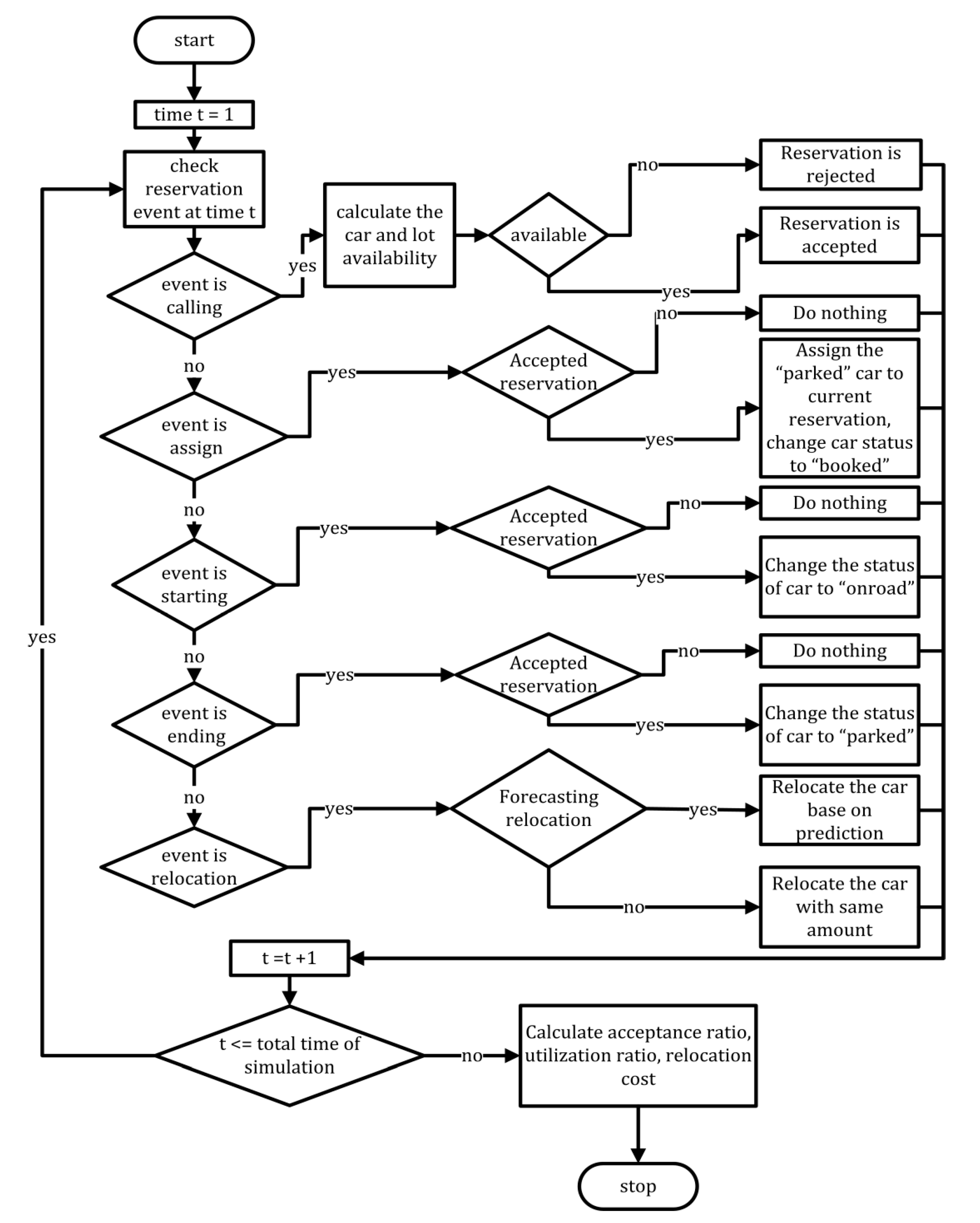
The simulation program reads the reservation data from the earliest to the last hour of the simulation. The program checks the RESERVATION_EVENT (calling, assign, starting, ending, or relocation) and does the task based on the identified event.
Figure 5 shows the simulation flowchart.
The program checks , the event status of reservation i at time t. There are five possible cases for reservation status (RESERVATION_EVENT), as follows.
(i)
The system calculates the vehicle availability from the departure station and lot availability in the destination station. The vehicle availability at calling time
t in departure station
j is
where
is the real number of parked vehicles in departure station
j at time
t,
is the total number of vehicles scheduled to return to departure station
j at time
t, and
is the number of vehicles that are not available for use because they have been reserved (scheduled to be out) from departure station
j at time
t. If
(vehicle is available at the departure station) and
> 0 (available space at the destination station), then the reservation decision will be accepted (
), otherwise it will be rejected. For an accepted reservation, starting from
t until the simulation end of time,
n,
has 1 added and
has 1 subtracted. From the reservation
i ending time,
u, until
n simulation,
has 1 added, since the car is scheduled to be away from station
j at
t and arrive at station
k at
u for this particular reservation. The system also reserves one space at the station
k, that starts from
t for the reservation.
(ii)
The system finds a car, d, located in the departure station for reservation i at starting time h, () with parked status (). The system randomly selects a parked car and assigns it to the particular reservation (). Once the process finishes, the car status is changed from parked to booked, starting from t () until n (). The car status is changed to booked to prevent the car from being assigned to another reservation until the status of that particular car changes to parked again.
(iii)
Starting from t until n, and at departure station j are decreased by 1, and is increased by 1. At t, the car is no longer scheduled to be OUT or parked, but is being driven by the customer. The system also adds one available space at the departure station when the car leaves at t. Thus, the car status is changed from booked to on the road from t until n ().
(iv)
Once the customer trip ends, the system increments the parked cars at destination station k by 1, from t until n. The system also decreases VIN by 1 at the destination station from t until n. The car is not scheduled to arrive at the destination station at some future time, because it has already arrived at the destination station. The car status is also changed from on road to parked () and its current location is updated to the destination station () t until n.
(v)
The system implements the relocation model, relocating a number of cars, u, from an overstocked station j to an under stocked station k based on their relocation type ().
The matrices were implemented as multidimensional arrays in the C++ programming language, ensuring that simulation performance was maximized. At time n, the simulation shows an average car utilization ratio, reservation acceptance ratio, and relocation cost for a given scenario. Different scenarios were implemented for the total number of cars, number of reservations, and relocation type. The simulation results were then collected for analysis and performance evaluation.
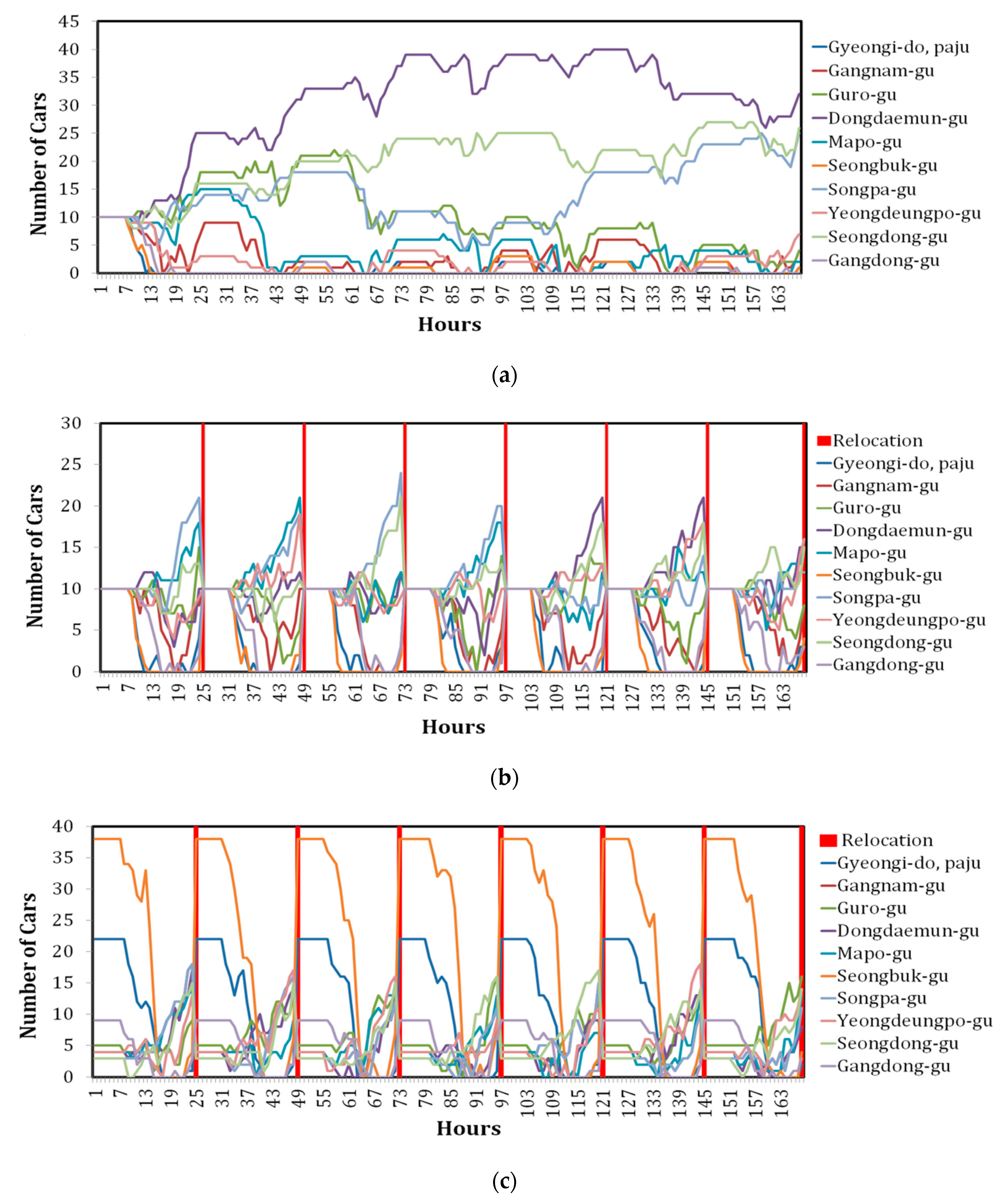
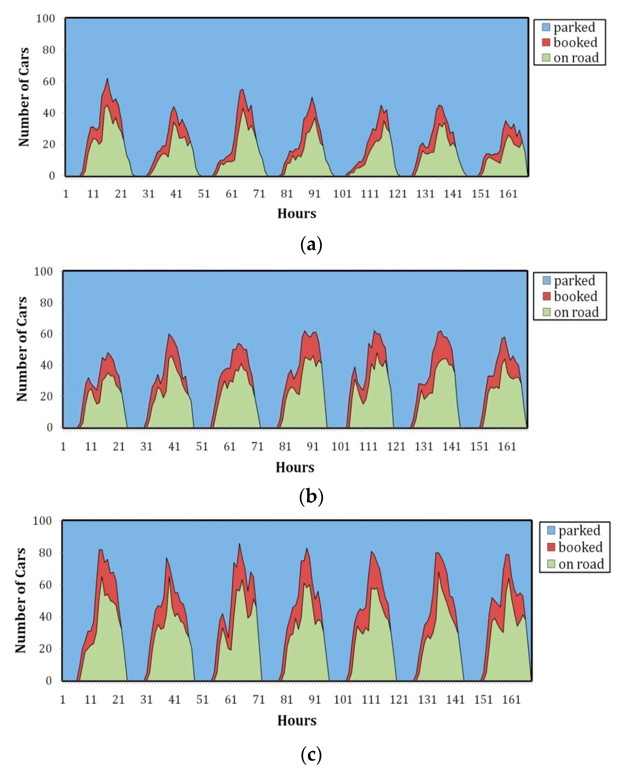
The program also provides the status of parked cars for all stations during the simulation on an hourly basis for the week, as shown in
Figure 6 for the case of 2800 total reservations in a week, 100 cars, and 10 stations.
Figure 6a shows an example of a non-relocation simulation where the initial number of parked cars was set as 10 cars in each station. The number of parked cars at each station is changed once the simulation is complete, and the unbalanced distribution is clear.
Figure 6b shows a rebalancing relocation with the same inputs. The number of parked cars at the various stations changes once the simulation is run. However, at midnight the rebalancing relocation is triggered, and the number of cars at each station resets to 10 cars again. Thus, to implement this model the operator needs to relocate approximately 30 cars per day.
Figure 6c shows forecasting relocation with the same inputs. However, the initial cars in each station was not set to be equal, but was based on prediction from the customer demand history. Thus, the number of cars initially at each station are different. Forecasting relocation is triggered at midnight, and the total number of cars in each station for the next day will be different based on customer demand at a particular station, calculated using the proposed MLP method. The relocation cost for this model was approximately 60 relocated cars per day.
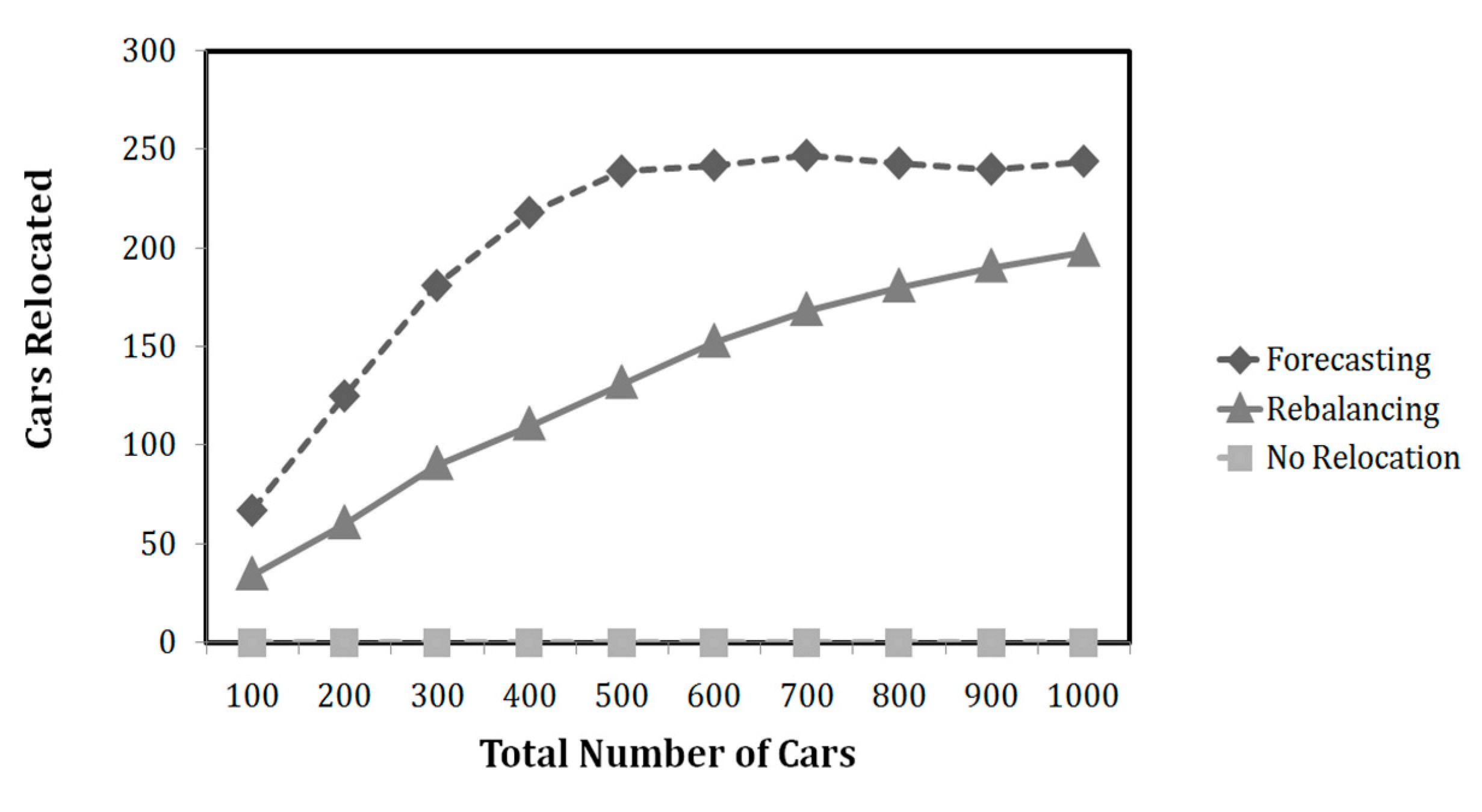
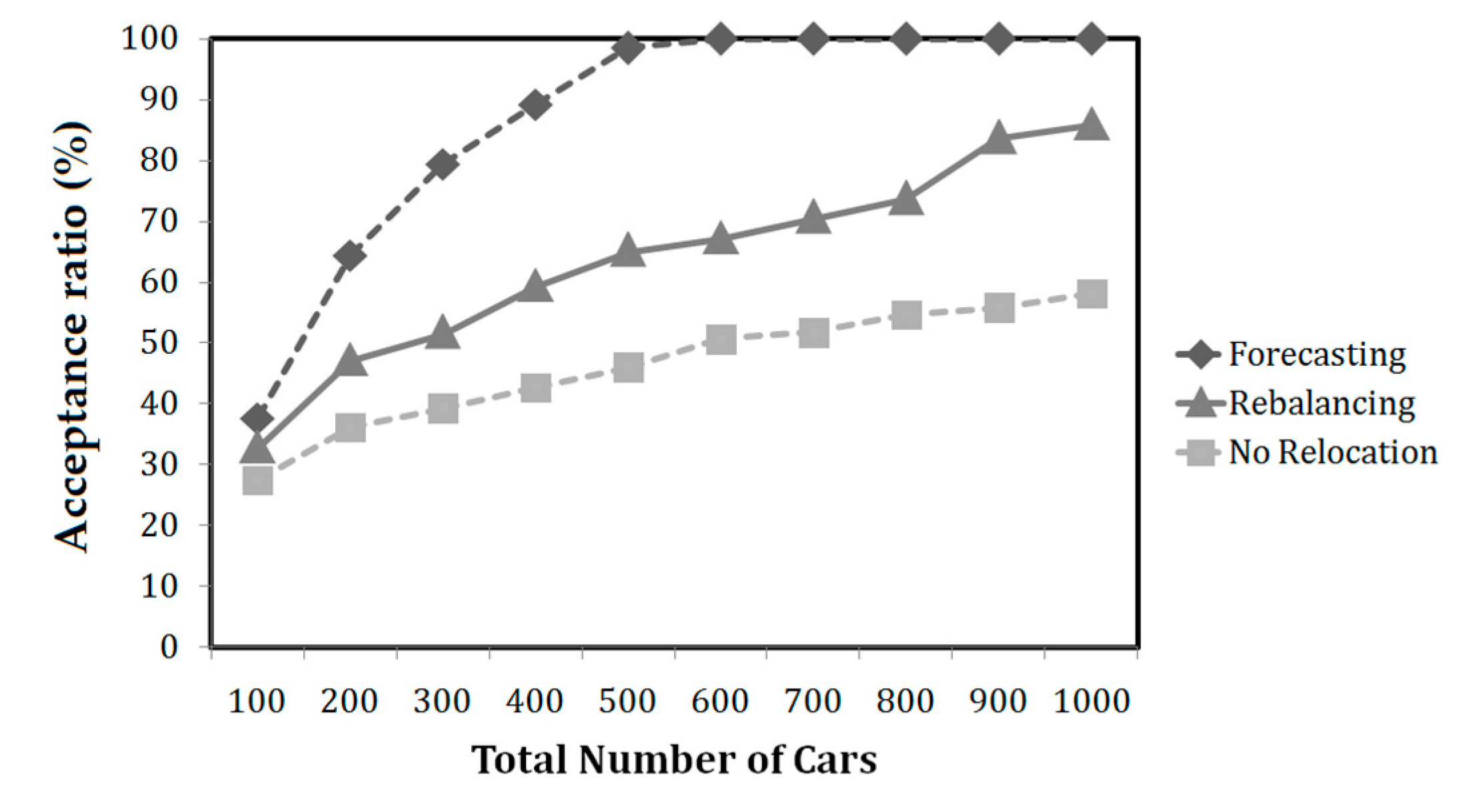
Figure 7 show the status of all 100 cars for each different simulation scenario. The total number of cars is a combination of booked, parked, and on road cars.
Figure 7a shows that omitting a relocation scheme results in a high number of parked cars and a low number of on road cars. Cars in each station become unbalanced, with most cars ending up in unpopular departure stations, and most customers (from high demand stations) are unable to make a reservation for the parked cars. The average car utilization was 14.32% with an acceptance ratio of 34.25%.
Figure 7b shows that rebalancing relocation reduced the number of parked cars, and increased the utilization and acceptance ratio to 19.31% and 47.6%, respectively.
Figure 7c shows that implementing forecasting relocation generates the lowest number of parked cars compared to the previous scenarios, and achieves the highest acceptance and utilization ratios, 26.95% and 67.53%, respectively.


 ,
, 

