Optimal Control of Drug Therapy in a Hepatitis B Model

Abstract

Combination antiviral drug therapy improves the survival rates of patients chronically infected with hepatitis B virus by controlling viral replication and enhancing immune responses. Some of these drugs have side effects that make them unsuitable for long-term administration. To address the trade-off between the positive and negative effects of the combination therapy, we investigated an optimal control problem for a delay differential equation model of immune responses to hepatitis virus B infection. Our optimal control problem investigates the interplay between virological and immunomodulatory effects of therapy, the control of viremia and the administration of the minimal dosage over a short period of time. Our numerical results show that the high drug levels that induce immune modulation rather than suppression of virological factors are essential for the clearance of hepatitis B virus.

1. Introduction

Hepatitis B virus (HBV) is the leading viral cause of liver disease, affecting 250–350 million people worldwide. Chronic HBV leads to the development of liver cirrhosis and liver cancer [1]. Despite the availability of effective HBV vaccination [2], the prevalence of chronic HBV has only marginally declined [3,4]. The natural course of chronic HBV includes an immune-tolerant phase, hepatitis B e-antigen positive immuno-active and -inactive phases and a hepatitis B e-antigen negative immuno-active phase [5]. Understanding the virological and immunological characteristics of each of these stages can provide a useful framework for the management of chronic HBV [6,7].

Currently, seven drugs have been approved for treating chronic HBV disease: standard and PEGylated interferon (IFN-α) and five nucleo(t)side analogs (NAs) [8]. These medications suppress HBV replication and liver inflammation, but do not lead to cure. The interferon-α treatments modulate immune responses that may lower viral levels. It is given for a finite time (usually 12 months) due to its toxic side effects [8,9]. The nucleo(t)side analogues are administrated for many years and sometimes for life and are responsible for viral suppression. However, life-long therapy is difficult due to costs, side effects, compliance and, most importantly, the development of antiviral drug resistance [10]. Combination therapy has not shown an increased effect on treatment response (but has reduced the rate of drug resistance) [11]. This has made it difficult to establish a universal guideline for treatment start, duration, which type or combinations of drugs to use [7] and how to define the success of therapy (virologically, serologically and/or immunologically) [7,12].

To provide insight into the optimal combination therapy and, in particular, into the immune-mediated effects of interferon-α, we design an optimal control study for a mathematical model of hepatitis B infection. Mathematical models have been used to address transition from acute to chronic HBV infections [13,14,15,16] and to study the effects of drug therapy [17,18,19]. Optimal control theory was developed by Pontryagin et al. for obtaining necessary conditions to characterize optimal controls for systems of ordinary differential equations (ODEs) [20]. Optimal control models have been used previously to design treatment strategies for disease models described by systems of ordinary differential equations with no delays [21,22,23,24,25] and systems of delay differential equations (DDEs) [26]. Kharatishvili [27] developed the extension of the Pontryagin’s maximum principle for systems of DDEs with constant time delays. For approximation and numerical methods for such problems, see [28,29].

In this paper, we modify an in-host DDE model of immune responses to hepatitis B infection introduced in [14] by adding the effects of combination drug therapy. In particular, we consider the drug effects in blocking viral production, reducing viral infection, enhancing the killing of infected cells by immune responses and removing immune cell exhaustion. We will use this as a starting model for designing an optimal control problem that advises what is the best combination therapy to ensure viral clearance, immune activation and the least amount of liver damage. Time-varying rates for therapies will be the controls in the system. Optimal control has been applied to the study of hepatitis B therapy using ODE [30,31] and DDE [32] models that did not consider an immune system component and using an ODE model that considers the enhancement of immune responses following administration of traditional Chinese medicine [33].

Here, we introduce the DDE system with constant time delay from [14], derive its corresponding control formulation and use it to determine the temporal, quantitative and qualitative effects of the drugs that lead to hepatitis B virus control, balancing the goals of reducing viral load and minimizing the negative side effects of therapy. Our results indicate that early drug therapy that mainly modulates and restores the immune responses against the virus is mandatory for the success of the therapy.

2. Mathematical Model and Analysis

2.1. Model of Hepatitis B Virus (HBV) Drug Therapy

To understand the various modes of action of antiviral therapy, we modify the model of acute infection published in [14] by considering the combined effects of NAs and interferon-α drugs. As in [14], we consider five state variables, corresponding to uninfected hepatocytes (T), productively-infected hepatocytes (I), free virus (V), immune effector cells (E) and a population of refractory hepatocytes (R).

All hepatocyte populations, uninfected, infected and refractory to reinfection, are maintained by homeostasis described by a logistic equation, with carrying capacity K and maximal per capita growth rate r. Virus infects target cells at rate β. Infected cells are killed by the immune responses at rate μ. As in [14], we assume that infected cells can be lost due to the non-cytolytic response at rate ρ, dependent on the effector cell population E [34], and move into a refractory class R. Refractory cells will still be assayed as infected, since surface antigens persist for some time [35]. We assume that they have lost their viral replicates and do not produce virus, which also makes them poor targets for cytotoxic T lymphocyte (CTL) responses. Therefore, the refractory population will be killed at a smaller rate, $\nu <\mu$. The refractory state is not permanent, and the R population may eventually become susceptible to reinfection. We model this by allowing R cells to move into the uninfected population at rate q. Free virus is produced at rate π and cleared at rate c.

In the absence of infection, we assume the immune effector cells E are at equilibrium value $s/d$, where s corresponds to a source of effector cells specific for HBV and $1/d$ is their average life-span. Upon encountering antigen (on the surface of infected liver cells), these cells expand at rate α, with a constant time delay τ accounting for the lag between antigen encounter and effector cell expansion.

We model drug therapy as interference with virus production and infection and as immune modulation, as follows. The contributions of interferon-α are complex, with both direct antiviral and immunomodulatory effects. Here, we consider three effects of IFN-α: enhancement of effector cell killing rates, reduction of viral production rate and the delay of effector cell programmed death [36,37]. We model this by changing rates μ, π and d to ${\mu }_1=\mu (1+a_1ϵ)$, ${\pi }_1^0=\pi (1-a_2ϵ)$ and $d_1=d(1-a_3ϵ)$, respectively. In each case, $0\le ϵ\le 1$ represents the efficacy of IFN-α, and $a_i\ge 0$ are scalar parameters representing the strength of the corresponding effect of interferon. $a_1$ can be any nonnegative number, while $a_2$ and $a_3$ are between 0 and 1.

The nucleos(t)ide analogues, on the other hand, interfere with both the ability of virus to infect a cell and with the generation of HBV DNA by an infected cell [38]. We model this by assuming that the infectivity rate in the presence of NAs becomes ${\beta }_1=\beta (1-b_1\eta )$, and the viral production rate becomes ${\pi }_1=\pi (1-f{a}_2ϵ-(1-f)b_2\eta )$. Here, $0\le \eta \le 1$ represents NAs’ efficacy; $b_i\ge 0$ are scalar parameters representing the relative strength of the corresponding effect of NAs; and f and $1-f$ represent the relative contribution of interferon-α and NAs, respectively, to reducing viral production, for $0\le f\le 1$.

For $t>t_d$, where $t_d$ represents the time of therapy onset, the dynamics of these populations is governed by the following differential equations

$$\begin{array}{c}\frac{dT}{dt}=rT\left(1-\frac{T+I+R}{K}\right)-(1-b_1\eta )\beta TV+qR\hfill \\ \frac{dI}{dt}=rI\left(1-\frac{T+I+R}{K}\right)+(1-b_1\eta )\beta TV-((1+a_1ϵ)\mu +\rho )IE\hfill \\ \frac{dV}{dt}=\pi (1-f{a}_2ϵ-(1-f)b_2\eta )I-cV\hfill \\ \frac{dE}{dt}=s+\alpha I(t-\tau )E(t-\tau )-d(1-a_3ϵ)E\hfill \\ \frac{dR}{dt}=\rho IE+rR\left(1-\frac{T+I+R}{K}\right)-qR-\nu RE\hfill \end{array}$$

(1)

As this is a system of delay differential equations with fixed delay τ, the initial conditions for the system are defined on the interval $[t_d-\tau ,t_d]$ by functions:

$$T\left(t\right)>0,V\left(t\right)\ge 0,R\left(t\right)\ge 0,I\left(t\right)\ge 0\mathrm{and}E\left(t\right)\ge 0$$

(2)

In many cases, these will be assumed to be constant and equal to the value of the state variables at $t=t_d$.

2.2. Model Analysis

We will consider that therapy leads to viral removal and only investigate the long-term behavior of the equilibrium where $V=0$. Model (1) has such a disease free steady state, $S_0=(K,0,0,s/d_1,0)$. In the absence of delay ($\tau =0$), the Jacobian matrix associated with (1) is:

$$\left[\begin{array}{ccccc}r(1-\frac{2T+I+R}{K})-{\beta }_{1}V& -\frac{rT}{K}& -{\beta }_{1}T& 0& q-\frac{rT}{K}\\ -\frac{rI}{K}+{\beta }_{1}V& r(1-\frac{T+2I+R}{K})-(\rho +{\mu }_1)E& {\beta }_{1}T& -\rho I-{\mu }_{1}I& -\frac{rI}{K}\\ 0& {\pi }_1& -c& 0& 0\\ 0& \alpha E& 0& \alpha I-d_1& 0\\ -\frac{rR}{K}& -\frac{rR}{K}+\rho E& 0& \rho I-\nu R& r(1-\frac{T+I+2R}{K})-q-\nu E\end{array}\right]$$

We evaluate $J\left(S_0\right)$ and obtain the Jacobian matrix:

$$J\left(S_0\right)=\left[\begin{array}{ccccc}-r& -r& -{\beta }_{1}K& 0& q-r\\ 0& -(\rho +{\mu }_1)s/d_1& {\beta }_{1}K& 0& 0\\ 0& {\pi }_1& -c& 0& 0\\ 0& \alpha s/d_1& 0& -d_1& 0\\ 0& \rho s/d_1& 0& 0& -q-\nu s/d_1\end{array}\right]$$

and the characteristic equation:

$$(r+\lambda )({\lambda }^4+A_1{\lambda }^3+A_2{\lambda }^2+A_3\lambda +A_4)=0$$

where

$$\begin{array}{cc}\hfill A_1& =c+d_1+q+(\rho +{\mu }_1+\eta )\frac{s}{d_1}\hfill \\ \hfill A_2& =\frac{s}{d_1}\left(\nu (c+d_1)+({\mu }_1+\rho )(d_1+q+\eta \frac{s}{d_1})\right)+q{d}_1+c{d}_1+qc+\left(c({\mu }_1+\rho )\frac{s}{d_1}-{\pi }_1{\beta }_{1}K\right)\hfill \\ \hfill A_3& =\frac{s}{d_1}(b{d}_{1}q+c{d}_1\nu +\rho d_{1}q+\nu s(\rho +{\mu }_1))+c{d}_{1}q+\left(d_1+q+\nu \frac{s}{d_1}\right)\left(c({\mu }_1+\rho )\frac{s}{d_1}-{\pi }_1{\beta }_{1}K\right)\hfill \\ \hfill A_4& =d_1(q+\nu \frac{s}{d_1})\left(c({\mu }_1+\rho )\frac{s}{d_1}-{\pi }_1{\beta }_{1}K\right)\hfill \end{array}$$

(3)

By the Routh–Hurwitz criteria, the characteristic equation has roots with negative real parts if and only if $A_i>0$, $A_1{A}_2-A_3>0$ and $A_1{A}_2{A}_3-A_3^2-A_1^2{A}_4>0$. We can show that these conditions are satisfied when $A_4>0$.

Therefore, when $\tau =0$, $S_0$ is locally asymptotically stable when:

$$\frac{{\pi }_1{\beta }_{1}K{d}_1}{c({\mu }_1+\rho )s}=\frac{(1-b_1\eta )(1-f{a}_2ϵ-(1-f)b_2\eta )(1-a_3ϵ)\pi \beta Kd}{(a_1ϵ\mu +\mu +\rho )cs}<1$$

(4)

and is unstable otherwise. This condition gives us a minimal drug efficacy for viral clearance in the absence of delay in immune activation.

When $\tau >0$, the characteristic equation at state $S_0$ is:

$$det(B+e^{-\lambda \tau }C-\lambda I_5)=0$$

(5)

where:

$$B=\left[\begin{array}{ccccc}-r& -r& -{\beta }_{1}K& 0& q-r\\ 0& -(\rho +{\mu }_1)s/d_1& {\beta }_{1}K& 0& 0\\ 0& {\pi }_1& -c& 0& 0\\ 0& 0& 0& -d_1& 0\\ 0& \rho s/d_1& 0& 0& -q-\nu s/d_1\end{array}\right]$$

and:

$$C=\left[\begin{array}{ccccc}0& 0& 0& 0& 0\\ 0& 0& 0& 0& 0\\ 0& 0& 0& 0& 0\\ 0& \alpha s/d_1& 0& 0& 0\\ 0& 0& 0& 0& 0\end{array}\right]$$

We see that the transcendental Equation (5) reduces to polynomial:

$$(r+\lambda )({\lambda }^4+A_1{\lambda }^3+A_2{\lambda }^2+A_3\lambda +A_4)=0$$

as in the $\tau =0$ case. Therefore, the infection-free equilibrium $S_0$ is locally asymptotically stable for all τ when (4) holds.

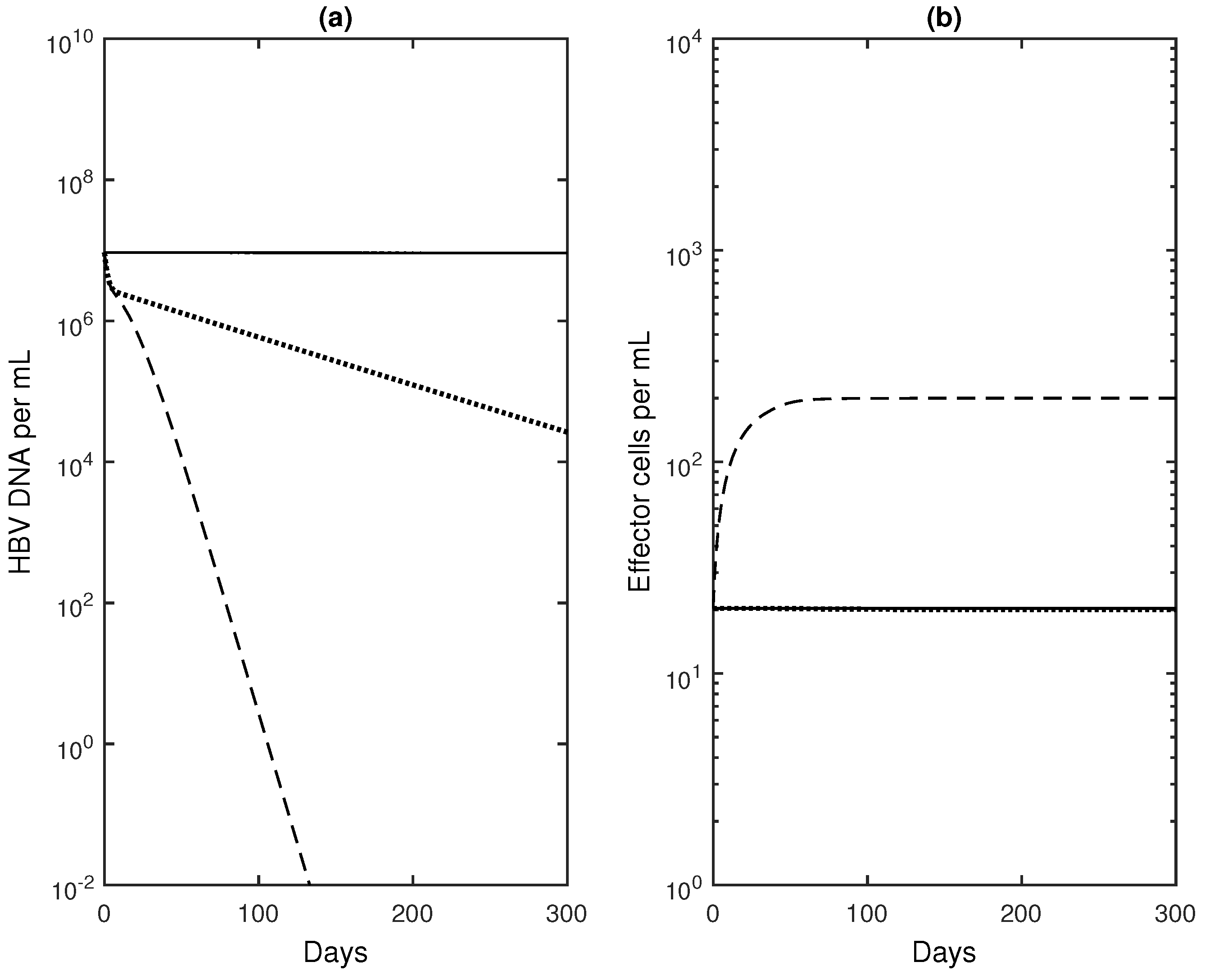
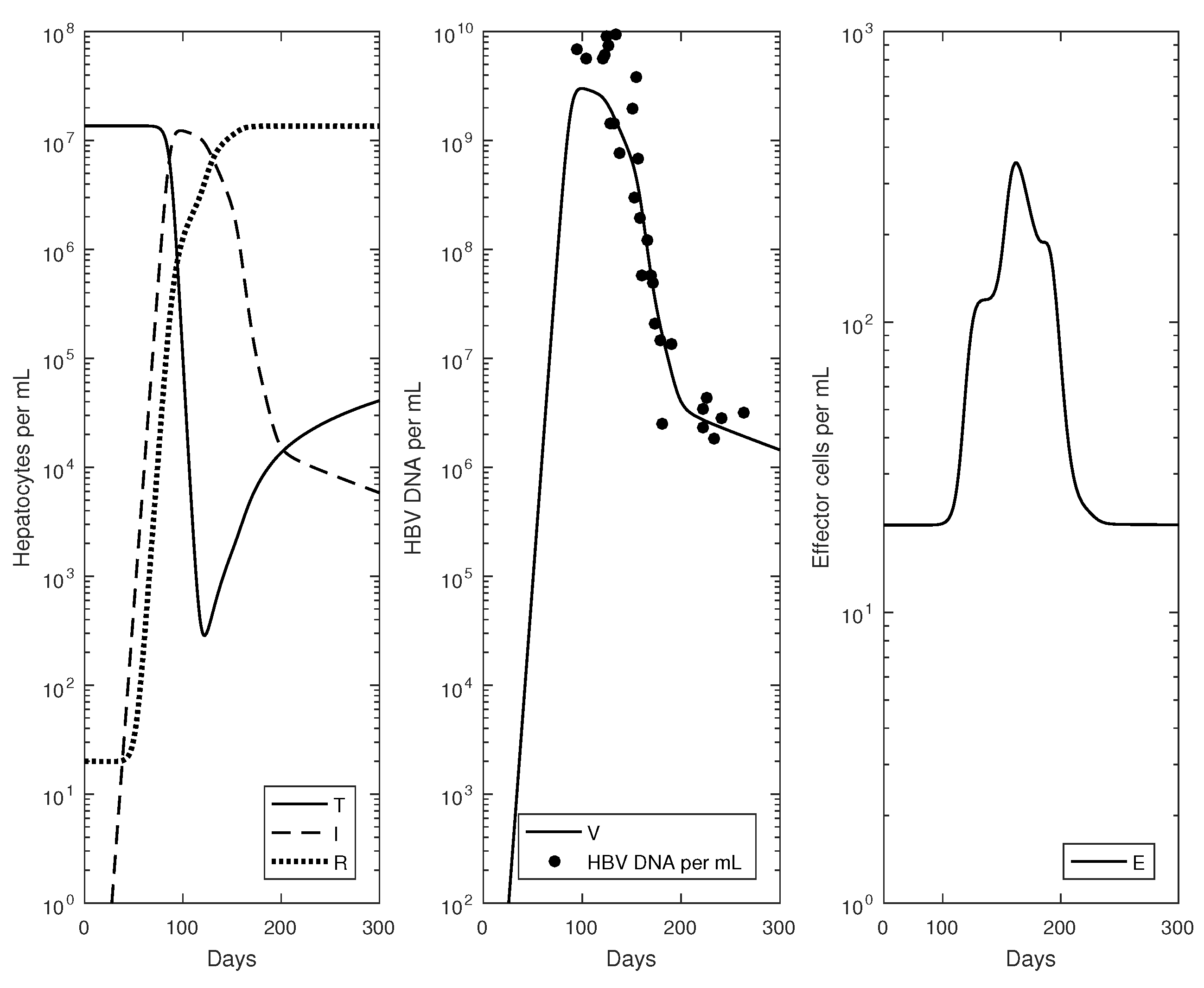
2.3. Numerical Results

We assume that in the absence of drug therapy, the virus will persist, and the patient will experience chronic infection. We therefore set all parameters values and initial conditions to the values for the chronically-infected Patient 7 in [14] (see

Table 1. Variables, parameters and values used in simulations with mililiter (mL) and day (d).

Variables
T	Target cells	$T_0=13.6\times {10}^6$ per mL
I	Infected cells	$I_0=0$ per mL
V	Free virus	$V_0=0.33$ per mL
E	Effector cells	$E_0=60$ per mL
R	Refractory cells	$R_0=0$ per mL
Parameters
r	Hepatocyte maximum proliferation rate	1 day${}^{-1}$
β	Infectivity rate constant	$1.22\times {10}^{-10}$ mL (virion × day)${}^{-1}$
K	Hepatocyte carrying capacity	$13.6\times {10}^6$ cells per mL
μ	Infected cell killing rate	$1.2\times {10}^{-4}$ mL (cell × day)${}^{-1}$
ν	Refractory cell killing rate	$1.27\times {10}^{-5}$ mL (cell × day)${}^{-1}$
ρ	Cure rate	$3.38\times {10}^{-4}$ mL (cell × day)${}^{-1}$
α	Effector cell expansion rate	$2\times {10}^{-7}$ mL (cell × day)${}^{-1}$
τ	Delay	$33.4$ days
π	Virus production rate	164 virion (cell × day)${}^{-1}$
c	Virus clearance rate	$0.67$ day${}^{-1}$
s	Effector cell production	10 day${}^{-1}$
d	Effector cell clearance rate	$0.5$ day${}^{-1}$
q	Waning of refractory cell immunity	$2\times {10}^{-5}$ day${}^{-1}$

). The dynamics of the five variables in the absence of drug therapy, $ϵ=\eta =0$, throughout acute infection and transition to chronic disease is presented in Figure 1.

We next investigate the change in the model dynamics in the presence of treatment. Initially, we set time-constant drug efficacy, $\eta =0.5$ and $ϵ=0.9$ as in [17]; assume scalars $a_i$ and $b_i$ to be either 1 or 0, representing an effect or lack of effect in therapy; and set $f=0.5$. We define HBV DNA clearance as the presence of less than one HBV DNA in the host serum. Since we assume that HBV DNA can distribute throughout the 3 liters of serum in an average 70-kg person, the viral extinction becomes $V\le V_{ext}=3\times {10}^{-4}$ copies per mL. We notice that the speed of viral extinction is dependent on both the timing of therapy initiation and on the type of effects considered.

Indeed, when the therapy is started at $t_d=T_{peak}=96$ days post-infection (corresponding to the peak HBV DNA), our model predicts HBV DNA clearance 145 days after the start of therapy when $a_1=a_2=a_3=b_1=b_2=1$ and $f=0.5$ (see Figure 2a, dashed line) and 2226 days ($6.1$ years) after the start of therapy when $a_1=a_2=b_1=b_2=1$, $a_3=0$ and $f=0.5$ (see Figure 2a, dotted line). This suggests that the immune modulation effect of interferon is important in clearing the HBV DNA in a short amount of time.

Similar immune-mediated effects of interferon are observed when drug therapy is started at the chronic state of Model (1), $t_d=T_{ss}=20$ years post-infection. Indeed, viremia clearance occurs faster when $a_1=a_2=a_3=b_1=b_2=1$ and $f=0.5$ (see Figure 3a, dashed line) than when $a_1=a_2=b_1=b_2=1$, $a_3=0$ and $f=0.5$ (see Figure 3a, dotted lines). However, viral clearance is delayed by 12 days compared to the case in which therapy is initiated at peak HBV DNA. The rapidity of clearance during peak therapy is due to the transient effects of immune cells, which are activated and expanding at the peak HBV DNA (see Figure 2b, solid lines) and tolerant at the chronic HBV infection (see Figure 3b, solid lines).

These results are supported by relative sensitivity curves. Briefly, sensitivity functions are numerical solutions of the following system:

$$\begin{array}{cc}\hfill & \frac{dx}{dt}=g(x(t,\xi ),z(t,\xi ),\xi )\hfill \end{array}$$

(6)

$$\begin{array}{cc}\hfill & \frac{d}{dt}\frac{\partial x}{\partial \xi }=\frac{\partial g}{\partial x}\frac{\partial x}{\partial \xi }+\frac{\partial g}{\partial z}\frac{\partial z}{\partial \xi }+\frac{\partial g}{\partial \xi }\hfill \end{array}$$

(7)

where $x(t,\xi )=\left(T\right(t,\xi ),I(t,\xi ),V(t,\xi ),E(t,\xi ),R(t,\xi \left)\right)$, $z(t,\xi )=x(t-\tau ,\xi )\in {\mathbb{R}}^5$, the function g represents the right-hand side of Model (1) and:

$$\xi =\left(r,K,\beta ,q,\rho ,\pi ,c,s,\alpha ,d,\eta ,\nu ,\mu ,ϵ,a_1,a_2,a_3,b_1,b_2,f\right)$$

The partial derivatives $\partial x_i/\partial {\xi }_j$, for $i=1,\cdots ,5$ and $j=1,\cdots ,20$, are time functions denoting the rate of change in a state variable with respect to variations in model parameters (see [39] and the references therein). The functions ${\xi }_j/x_i\times \partial x_i/\partial {\xi }_j$ are the relative sensitivity curves (similar to relative error), which allow for the comparison between the sensitivity of two variables $x_i^1$ and $x_i^2$ with respect to the same parameter ${\xi }_j$. Here, we are interested in the sensitivity of $V(t,\xi )$ and $E(t,\xi )$ with respect to model parameters $\xi =\{a_2,a_3,b_2\}$. As the numerical solutions displayed in Figure 4 show, the $a_3$ effect is the most important drug effect in both reducing virus load and increasing immune response.

Our model suggests that the timing and the type of interferon effects are important in the success of the treatment. In the next sections, we will consider a time-dependent effect of both interferon and nucleo(s)tide analogues, and we will formulate an optimal control problem for our model to determine the connection between successful therapy and the optimal temporal efficacy of the effects considered.

3. Optimal Control Problem

To better understand the interactions between drug therapy and the host immune reaction, we allow the effects of the two drug types (NAs and IFN-α) to vary with time. We replace the NAs’ efficacy parameter η with $u_1\left(t\right)$ to represent the time-varying effective drug dosage needed for optimal therapy. Similarly, $u_2\left(t\right)$ will replace the parameter ϵ to represent the time-varying dosage of IFN-α. As before, $a_1$, $a_2$ and $a_3$ indicate the relative strength of the three effects of IFN-α under consideration; $b_1$ and $b_2$ represent the relative strengths of the two effects of the NA; and f and $1-f$ are the relative contribution of interferon and NAs, respectively, in reducing viral production.

For computational convenience and consistency of notation, we will relabel the state variables as in

Table 2. Correspondence between labeling of the state variables in Models (1) and (8).

$x_1\left(t\right)=T\left(t\right)$
$x_2\left(t\right)=I\left(t\right)$	$z_2\left(t\right)=I(t-\tau )$
$x_3\left(t\right)=V\left(t\right)$
$x_4\left(t\right)=E\left(t\right)$	$z_4\left(t\right)=E(t-\tau )$
$x_5\left(t\right)=R\left(t\right)$

. With these adjustments, our model becomes as follows.

$$\begin{array}{cc}\hfill \frac{d{x}_1}{dt}& =r{x}_1\left(1-\frac{x_1+x_2+x_5}{K}\right)-\beta (1-b_1{u}_1)x_1{x}_3+q{x}_5\hfill \\ \hfill \frac{d{x}_2}{dt}& =r{x}_2\left(1-\frac{x_1+x_2+x_5}{K}\right)+\beta (1-b_1{u}_1)x_1{x}_3-((1+a_1{u}_2)\mu +\rho )x_2{x}_4\hfill \\ \hfill \frac{d{x}_3}{dt}& =(1-f{a}_2{u}_2-(1-f)b_2{u}_1)\pi x_2-c{x}_3\hfill \\ \hfill \frac{d{x}_4}{dt}& =s+\alpha z_2{z}_4-d(1-a_3{u}_2)x_4\hfill \\ \hfill \frac{d{x}_5}{dt}& =\rho x_2{x}_4+r{x}_5\left(1-\frac{x_1+x_2+x_5}{K}\right)-q{x}_5-\nu x_4{x}_5\hfill \end{array}$$

(8)

Our goal is to find the regime of drug therapy that minimizes the objective functional:

$$J(u_1,u_2)={\int }_0^T\left(c_1{x}_3+c_2{x}_2+c_3{u}_1+c_4{u}_2+{\epsilon }_1{u}_1^2+{\epsilon }_2{u}_2^2\right)dt+c_5{x}_3\left(T\right)$$

(9)

subject to the system of delay differential Equation (8) with initial conditions (2). Here, T represents the duration of therapy. We will study two different scenarios for drug treatment by considering two different sets of initial conditions. For the case of chronic HBV infection, the initial values of the state variables $x_i$ will be constant and equal to their chronic infection equilibrium values for the entire interval $[t_d-\tau ,t_d]$. We will also study the case of drug therapy initiation at the peak of viral load, during acute infection. In this case, the initial functions for the state variables $x_i$ will be set by their trajectories during acute infection in the absence of treatment. This is described in more detail in Section 3.3.

Given upper bounds $M_i$ on $u_i$ (for $i=1,2$), we seek to find an optimal pair in the control set:

$$U=\{(u_1,u_2)\in L^{\infty }(0,T)|0\le u_i\le M_i,i=1,2\}$$

such that

$$J(u_1^{*},u_2^{*})=\underset{(u_1,u_2)\in U}{inf}J(u_1,u_2)$$

The integral portion of the objective functional encapsulates the goal of minimizing total virus concentration ($x_3$), infected cell concentration ($x_2$) and the amount of drug used ($u_1$ and $u_2$ terms) over the entire treatment period. The final term $c_5{x}_3\left(T\right)$ represents the goal of minimizing the final viral concentrations at time T, which ideally would be below clearance levels. The parameters $c_i>0$ and ${\epsilon }_j>0$ give the relative weight of each of these factors.

3.1. Analysis of the Optimal Control Problem

Pontryagin’s key idea was to use adjoint functions to attach the state dynamics to the objective functional. This converts the problem into minimizing the Hamiltonian and generates the adjoint differential equations and final-time transversality conditions. In this paper, we use a generalization of Pontryagin’s maximum principle to systems of delay differential equations (developed by [27]).

Letting f denote the integrand of the objective functional (9) and $g_1,\dots ,g_5$ be the right-hand sides of System (8), the Hamiltonian for our optimal control problem is:

$$H=f+{\lambda }_1{g}_1+{\lambda }_2{g}_2+{\lambda }_3{g}_3+{\lambda }_4{g}_4+{\lambda }_5{g}_5$$

(10)

where the adjoint functions ${\lambda }_i$ correspond to the states $x_i$, for $i\in \{1,\dots ,5\}$.

From the Hamiltonian, we derive the adjoint equations. For $i=1$, 3 and 5, we have:

$$\frac{d{\lambda }_i}{dt}=-\frac{\partial H}{\partial x_i}$$

(11)

on $[0,T]$. For $i=2$ and 4, on the interval $[0,T-\tau ]$ we have

$$\begin{array}{cc}\hfill \frac{d{\lambda }_2}{dt}& =-\frac{\partial H}{\partial x_2}-{\left.\frac{\partial H}{\partial z_2}\right|}_{t+\tau }\hfill \\ \hfill \frac{d{\lambda }_4}{dt}& =-\frac{\partial H}{\partial x_4}-{\left.\frac{\partial H}{\partial z_4}\right|}_{t+\tau }\hfill \end{array}$$

(12)

where $z_i\left(t\right)=x_i(t-\tau )$ represent the delayed state variables, while on the interval $[T-\tau ,T]$, we have:

$$\begin{array}{cc}\hfill \frac{d{\lambda }_2}{dt}& =-\frac{\partial H}{\partial x_2}\hfill \\ \hfill \frac{d{\lambda }_4}{dt}& =-\frac{\partial H}{\partial x_4}\hfill \end{array}$$

(13)

just as in [11].

The equations containing delayed state variables produce adjoint equations with a “forward” delay, due to the opposite time orientation of the adjoint differential equation. The adjoint equations are subject to the final condition that ${\lambda }_3\left(T\right)=c_5$, ${\lambda }_i\left(T\right)=0$ and $i\in \{1,2,4,5\}$. On the interior of the control set, minimizing the Hamiltonian gives:

$$\frac{\partial H}{\partial u_i}=0$$

at $(u_1^{*},u_2^{*})$, and then, the optimal control pair becomes:

$$\begin{array}{cc}\hfill u_1^{*}& =\frac{-c_3+\beta x_1{x}_3(-{\lambda }_1+{\lambda }_2)+{\lambda }_3(1-f)b_2\pi x_2}{2{\epsilon }_1}\hfill \\ \hfill u_2^{*}& =\frac{-c_4+{\lambda }_2{a}_1\mu x_2{x}_4+{\lambda }_{3}f{a}_2\pi x_2-{\lambda }_{4}d{a}_3{x}_4}{2{\epsilon }_2}\hfill \end{array}$$

(14)

Using the bounds on the controls, we obtain the following characterization of the optimal control:

$$\begin{array}{cc}\hfill u_1^{*}& =min\left\{M_1,max\left\{0,\frac{-c_3+\beta x_1{x}_3(-{\lambda }_1+{\lambda }_2)+{\lambda }_3(1-f)b_2\pi x_2}{2{\epsilon }_1}\right\}\right\}\hfill \\ \hfill u_2^{*}& =min\left\{M_2,max\left\{\frac{-c_4+{\lambda }_2{a}_1\mu x_2{x}_4+{\lambda }_{3}f{a}_2\pi x_2-{\lambda }_{4}d{a}_3{x}_4}{2{\epsilon }_2}\right\}\right\}\hfill \end{array}$$

(15)

3.2. Implementation of the Optimal Control Problem

We wish to find optimal controls numerically by applying a forward-backward iterative method [25]. Initially, a constant control is assumed, and the state equations are solved in the forward-time direction from our standard set of initial conditions. Given this solution to the state equations, the adjoint equations are then solved in the backwards-time direction, beginning with the final time T and final condition ${\lambda }_3\left(T\right)=c_5$ and ${\lambda }_i\left(T\right)=0$ for $i\in \{1,2,4,5\}$. The controls to be used for the next forward run are then updated using the characterization of the optimal control given in (15), and the forward-backward solution process is repeated with the updated control functions. This process is iterated until the controls and the solutions to all of the differential equations converge to within acceptable numerical tolerances. See [28,29,40] for the background on this procedure and the approximation of delay equations.

To use the forward-backward sweep, we rewrite the adjoint equations for our system as:

$$\begin{array}{cc}\hfill \frac{d{\lambda }_1}{dt}=& -{\lambda }_1\left(r\left(1-\frac{2x_1+x_2+x_5}{K}\right)-(1-b_1{u}_1)\beta x_3\right)-{\lambda }_2\left(-\frac{r}{K}{x}_2+(1-b_1{u}_1)\beta x_3\right)+{\lambda }_5\frac{r}{K}{x}_5,\hfill \\ \hfill \frac{d{\lambda }_2}{dt}=& -c_2+{\lambda }_1\frac{r}{K}{x}_1-{\lambda }_2\left(r\left(1-\frac{x_1+2x_2+x_5}{K}\right)-(1+a_1{u}_2)\mu x_4-\rho x_4\right)\hfill \\ & -{\lambda }_3(1-(1-f)b_2{u}_1-f{a}_2{u}_2)\pi -{\lambda }_5\left(\rho x_4-\frac{r}{K}{x}_5\right)-{\lambda }_4(t+\tau )\alpha x_4{\chi }_{[0,T-\tau ]}\hfill \\ \hfill \frac{d{\lambda }_3}{dt}=& -c_1+{\lambda }_1(1-b_1{u}_1)\beta x_1-{\lambda }_2(1-b_1{u}_1)\beta x_1+{\lambda }_{3}c\hfill \\ \hfill \frac{d{\lambda }_4}{dt}=& -{\lambda }_2\left(-(1+a_1{u}_2)\mu x_2-\rho x_2\right)+{\lambda }_{4}d(1-a_3{u}_2)-{\lambda }_5(\rho x_2-\nu x_5)-{\lambda }_4(t+\tau )\alpha x_2{\chi }_{[0,T-\tau ]}\hfill \\ \hfill \frac{d{\lambda }_5}{dt}=& -{\lambda }_1\left(-\frac{r}{K}{x}_1+q\right)+{\lambda }_2\frac{r}{K}{x}_2-{\lambda }_5\left(r\left(1-\frac{x_1+x_2+2x_5}{K}\right)-q-\nu x_4\right)\hfill \end{array}$$

(16)

Notice that in the time interval $[T-\tau ,T]$, the advance terms (those with argument $t+\tau$, found in the second and fourth equations) drop out, so we have five ordinary differential equations. On the interval $[0,T-\tau ]$, we once again have advance equations, but the solutions to the ODEs on $[T-\tau ,T]$ provide the required initial data to solve these equations. Thus, the adjoint equations are advance differential equations on $[0,T-\tau ]$ and ordinary differential equations on $[T-\tau ,T]$, subject to the final condition ${\lambda }_3\left(T\right)=c_5$ and ${\lambda }_i\left(T\right)=0$ for $i\in \{1,2,4,5\}$.

For our numerical simulations, we used the built-in MATLAB numerical delay differential equation solver, dde23. This tool is not capable of solving advance equations directly, so we made a change of variables to convert the advance differential equations to a system of delay differential equations. Specifically, we define a new reversed-time variable $\sigma =T-t$ and new adjoint variables $L_i\left(\sigma \right)={\lambda }_i(T-\sigma )={\lambda }_i\left(t\right)$. In terms of these new variables, adjoint equations for $L_i\left(\sigma \right)$ are ordinary differential equations on $[0,\tau ]$ and delay differential equations on $[\tau ,T]$, subject to the initial condition $L_3\left(0\right)=c_5$ and $L_i\left(0\right)=0$ for $i\in \{1,2,4,5\}$. The new system was solved numerically using dde23 as part of the implementation of the forward-backward method to find the optimal control.

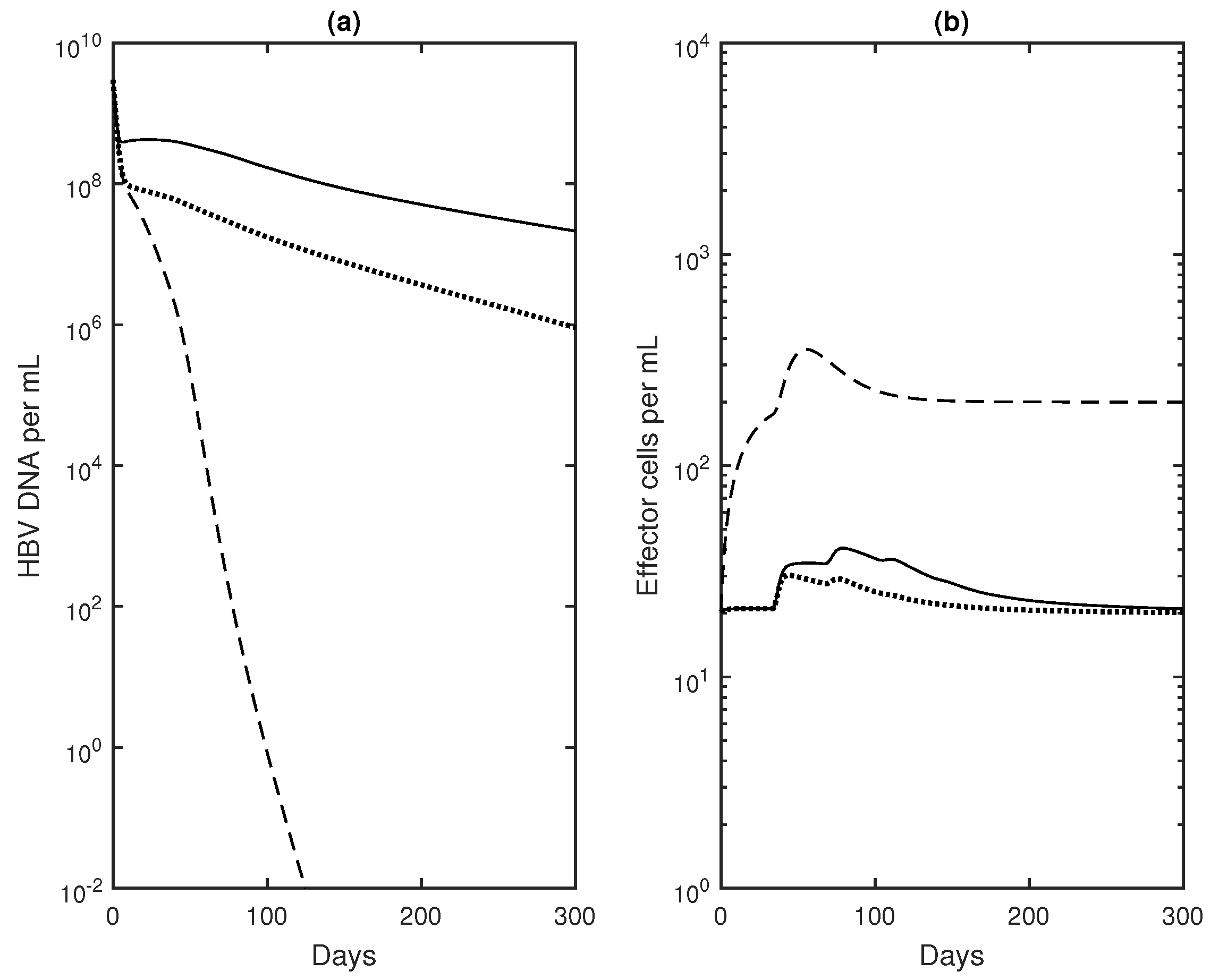
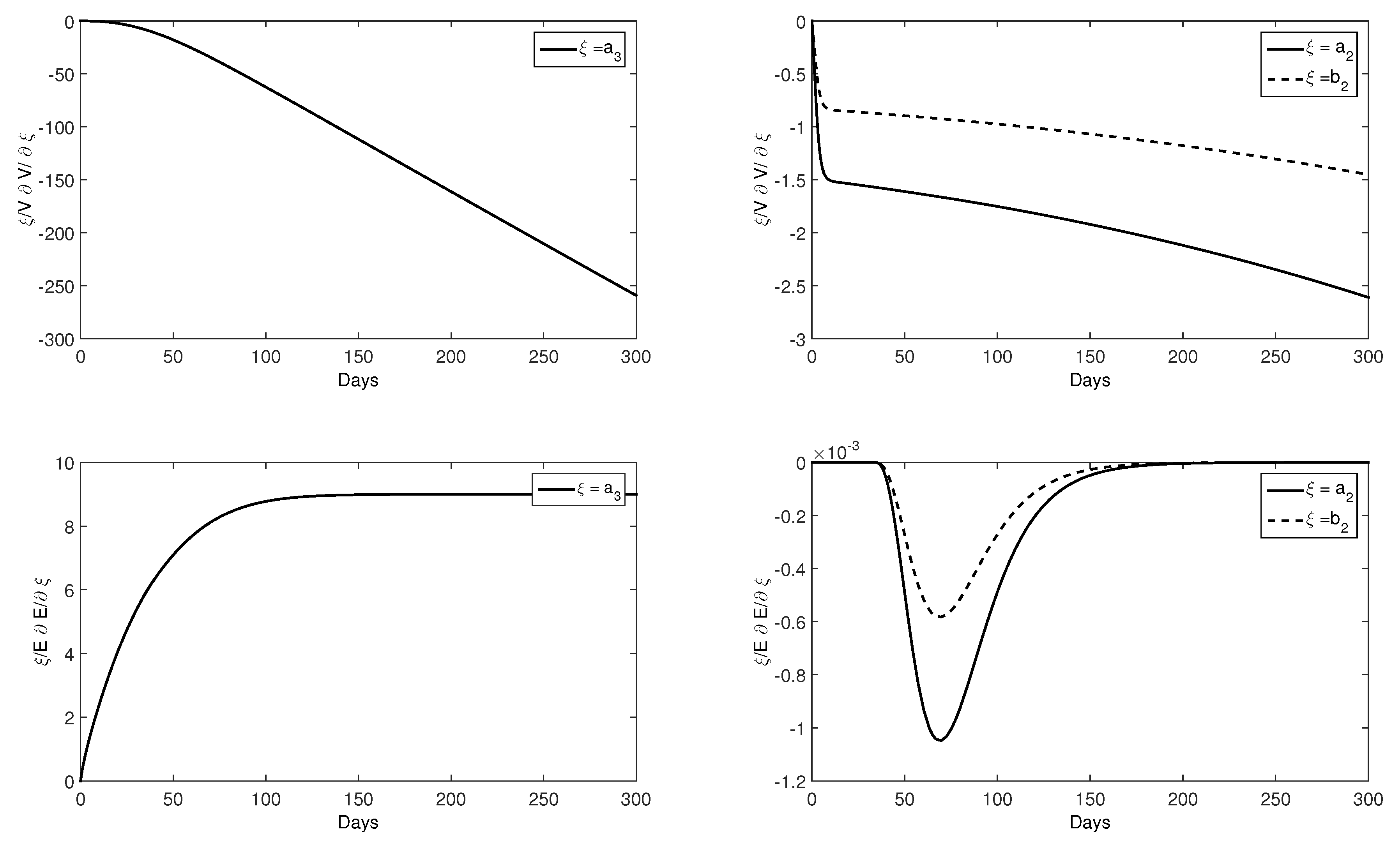
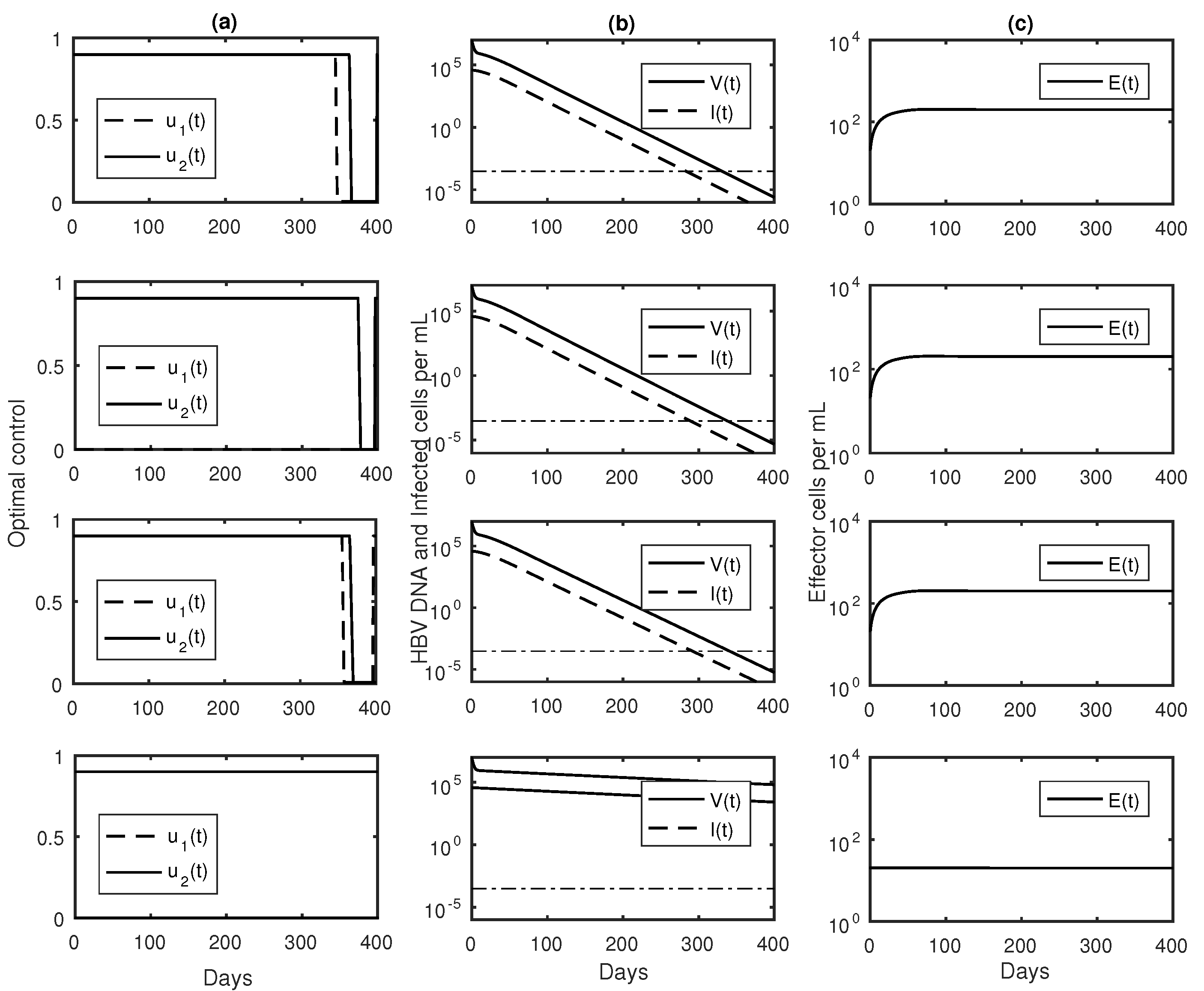
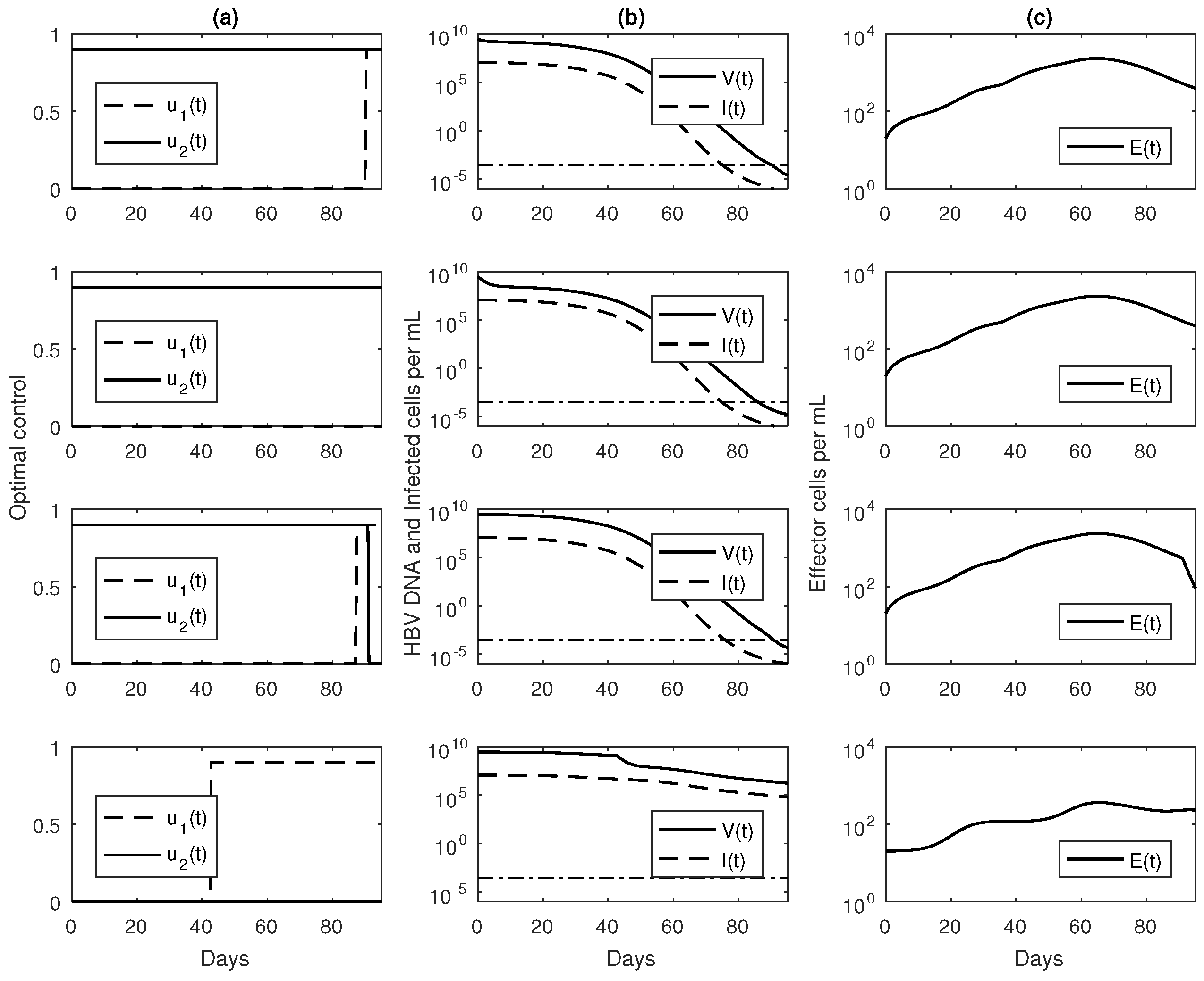
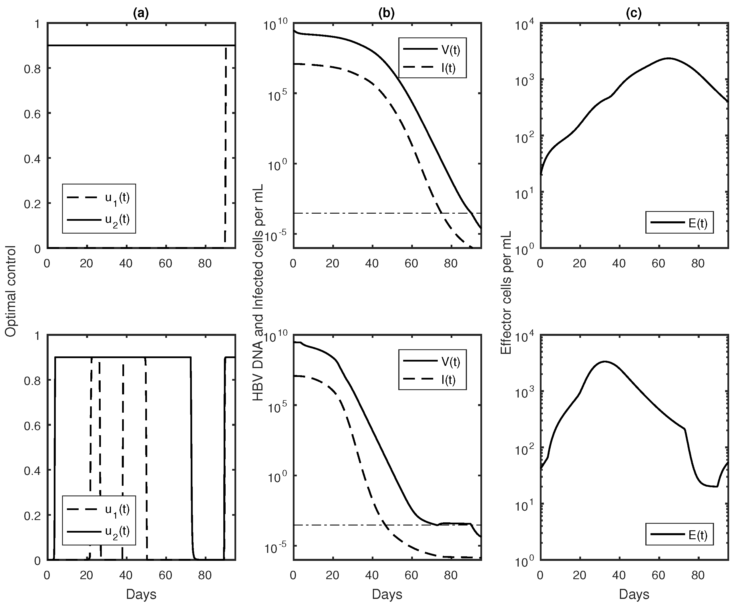
3.3. Numerical Results with Optimal Controls

For optimal therapy during chronic HBV infection, we assume that at the time of treatment initiation, the patient has reached chronic steady state values ${\overline{x}}_1=3\times {10}^5$ cells per mL, ${\overline{x}}_2=3.8\times {10}^4$ cells per mL, ${\overline{x}}_3=9.33\times {10}^6$ HBV DNA per mL, ${\overline{x}}_4=20.3$ cells per mL and ${\overline{x}}_5=1.33\times {10}^7$ cells per mL. The terms in the objective functional (9) have different scales. In order to weigh each term equally, we choose parameters $c_i$, such that $c_i{x}_i$ (for $i=1,2$) and $c_i{u}_i$ (for $i=3,4$) are one at the start of the optimal control. When the optimal control is started at the viral steady state, we normalize variables $x_1$ and $x_2$ by $c_1=\frac{1}{{\overline{x}}_3}$ and $c_2=\frac{1}{{\overline{x}}_2}=\frac{\pi }{c{\overline{x}}_3}$. As a result, the factors $c_1{x}_1$ and $c_2{x}_2$ are one at the beginning of treatment and between zero and one from there on. Since we assume $0\le u_1\left(t\right),u_2\left(t\right)\le 0.9$ for all t, their corresponding weights are $c_3=c_4=1$. Lastly, we choose the effects for the convex terms to be ${ϵ}_1={ϵ}_2=\mathbf{0}.\mathbf{1}$. The treatment will be given for $T_1=400$ days, which is sufficient for virus clearance and is still within the timeline of the HBV therapy guidelines [7].

The ideal clinical outcome of HBV drug therapy is to achieve viral suppression, such that $x_3\le V_{ext}=3\times {10}^{-4}$ HBV DNA per mL, corresponding to one HBV DNA in the body (as in Section 2.3). To account for this final condition, we set $c_5=3\times {10}^3$ so that the final time condition is normalized to one. Under these assumptions, we run the optimal control problem over $T_1=400$ days with the aim of finding the best temporal drug usage at each time point that ensures viral clearance while minimizing the drug levels.

We will be considering several scenarios by varying the levels of control effects, described by constants $a_i$ and $b_i$. Our simulations show that for high virus levels (above extinction), the optimal control will always be the maximal drug dosage for the scenario considered. For example, for a case with any $a_i>0$ and $b_1=b_2=0$, the optimal control is $u_1\left(t\right)=0$ and $u_2\left(t\right)=0.9$ for all time points. Similarly, if $a_i>0$ and $b_j>0$, then the optimal control is $u_1\left(t\right)=u_2\left(t\right)=0.9$ for all time points. Therefore, for the first 325 days, we assume the maximal drug dosage for a given scenario and only run the optimal control with variable $u_1\left(t\right)$ and $u_2\left(t\right)$ for the final 75 of the 400 days of treatment.

Initially, we include all effects of nucleos(t)ide analogues $u_1$ and interferon $u_2$, i.e., $a_1=a_2=a_3=b_1=b_2=1$ and $f=0.5$. For this choice of parameters, optimal control requires: (i) maximal NA drug dosage $u_1=0.9$ for $0\le t\le 347$ days and zero drug dosage for $t\ge 347$ days; and (ii) maximal $u_2=0.9$ interferon dosage for $0\le t\le 366.5$ days, zero dosage for $366.5\le t\le 399$ days and maximal dosage after that (see Figure 5a, top row). Under these drug regimes, HBV DNA is cleared 331 days after the start of treatment (see Figure 5b, top row).

We next assume monotherapy with interferon-α. We set $b_1=b_2=0$, $a_1=a_2=a_3=1$ and change the anti-viral production effect to $f=1$. The optimal control problem predicts that the virus is cleared 338 days after the start of therapy, seven days later than under combination therapy (see Figure 5b, second row). Another downside of this monotherapy is the need for interferon dosage to be maximal ($u_2=0.9$) for $0\le t\le 377$ and for $t\ge 396.5$ in order to compensate for the lack of NAs (see Figure 5a, second row).

In combination therapy, when $u_2$ neither increases CTLkilling abilities nor reduces virus production, i.e., $a_1=a_2=0$, and all other effects are maximal $a_3=b_1=b_2=1$, $f=0$ (so that NAs have maximal effect in blocking viral production), the HBV DNA will clear 341 days after the start of treatment (see Figure 5b, third row). The controls are: (i) $u_1=0.9$ for $0\le t\le 358$ and $t\ge 396$, and zero otherwise; and (ii) $u_2=0.9$ for $0\le t\le 369.5$, and zero otherwise (see Figure 5a, third row).

Lastly, we consider monotherapy with NAs alone. We set $a_1=a_2=a_3=0$, $b_1=b_2=1$ and $f=0$. The optimal control model does not result in viral clearance even when $u_1=0.9$ throughout the duration of the treatment (see Figure 5a,b, bottom row).

For the first three cases, we find that an increase in the effector cells’ lifespan is needed for viral suppression. Indeed, when $a_3=1$ and $u_2>0$, the increase of CTL lifespan to $1/d(1-a_3{u}_2)$ leads to elevated CTL concentrations (see Figure 5c, top three rows) and subsequent HBV DNA removal (see Figure 5b, top three rows). By contrast, when $a_3=0$, HBV DNA does not reach extinction during the $T_1=400$ days of therapy (see Figure 5b, bottom row) due to low HBV-tolerant CTL concentrations, $E=s/d_1=s/d$, which do not expand in the presence of HBV (see Figure 5c, bottom row).

For optimal therapy during acute HBV infection, to further determine the relationship between CTL activation and the possible success of short-term anti-HBV therapy, we run the optimal control problem during acute HBV disease, where CTL activation has been reported [41]. We start by running the DDE system mainly to the peak virus concentration occurring at time $T_{peak}$, record the values of all variables for the times $-\tau +T_{peak}\le t\le T_{peak}$ and start the optimal control problem at $t_d=T_{peak}$. The treatment will be given for $T_2=95$ days and, as before, we include the following weights $c_1=\frac{1}{x_3\left(T_{peak}\right)}$, $c_2=\frac{\pi }{c{x}_3\left(T_{peak}\right)}$, $c_3=c_4=1$, ${ϵ}_1={ϵ}_2=0.1$ and $c_5=3\times {10}^3$, so that all factors are normalized to one.

As in the chronic HBV case, we consider four scenarios. If we include all effects of nucleos(t)ide analogues $u_1$ and all effects of interferon $u_2$, i.e., $a_1=a_2=b_1=b_2=1$, $f=0.5$ and $a_3=0.9$, we predict that HBV DNA is cleared 90 days after the start of treatment when interferon dosage is maximal at each time step and NAs are zero for $0\le t\le 90$ days and maximal from $t\ge 90$ (see Figure 6a,b, top row). This result implies that NAs do not have a role in viral clearance. This is corroborated by the optimal control solution for interferon monotherapy. Indeed, when we set $a_1=a_2=1$, $a_3=0.9$, $b_1=b_2=0$ and $f=1$, virus is cleared even faster, 87 days after the start of therapy (see Figure 6b, second row) when $u_2$ dosage is maximal $u_2=0.9$ at each time step (see Figure 6a, second row). This is due to the higher efficacy of interferon-α at blocking viral production assumed in this scenario. The results in both of these cases are due to fast expansion and transient maintenance of CTLs to high levels of 2500 cells per mL (see Figure 6c, top two rows).

To further determine which of the interferon effects are the most influential, we remove the first two interferon effects $a_1=a_2=0$, keep $a_3=0.9$, $b_1=b_2=1$ and set $f=0$. Under these conditions, virus is cleared 91 days after the start of therapy, one and four days later than the previous two cases (see Figure 6b, third row) when: (i) NA dosage ($u_1$) is zero for $0\le t\le 87$ and maximal ($u_1=0.9$) afterwards; and (ii) interferon dosage is maximal ($u_2=0.9$) for $0\le t\le 91$ and zero afterwards (see Figure 6a, third row). This result implies, again, that interferon is needed for virus clearance.

Lastly, when we consider monotherapy with NAs, i.e., $b_1=b_2=1$, $a_1=a_2=a_3=0$ and $f=0$, the HBV DNA will not clear (see Figure 6b, bottom row) in spite of CTL levels being higher than the base of $E=s/d_1=s/d$ (see Figure 6c, bottom row). Interestingly, our numerical results show that the optimal NA dosage for the first 42 days is zero (see Figure 6a, bottom row).

Our study has used a delay of $\tau =33.4$ days, since that represented the delay in the CTL activation in the only patient that developed chronic disease in [14]. To check whether the size of the delay affects the results, we have investigated the optimal control problem for a shorter delay of $\tau =15.2$ days, which is the smallest delay among the patients in [14]. We found that the length of the delay does not influence the results when the therapy is started at the viral steady state (not shown). When the therapy is started at the peak viral load, we find, not surprisingly, that a shorter time lag speeds viral decay and CTL expansion (see Figure 7b,c). Moreover, the optimal control problem for the shorter delay of $\tau =15.2$ days suggests no therapy ($u_1=u_2=0$) for the first three days post-peak, maximal interferon therapy for $3\le t\le 75$ and $t\ge 90$ and no interferon $u_2=0$ otherwise. The role of NAs is transient, with maximal dosages $u_1=0.9$ for $20\le t\le 27$, $38\le t\le 51$ and $t>90$ days and $u_1=0$ elsewhere (see Figure 7a, bottom row).

Together, these results suggest that the immunomodulatory effects of interferon are needed for HBV DNA control and that immune modulation rather than suppression of virological factors is essential for inducing HBV clearance.

4. Discussion

The management of chronic hepatitis B is based on guidelines regarding screening, diagnosis, duration of treatment, adherence and monitoring of immune and virological markers [12]. Combined antiviral therapy improves the survival rates of patients chronically infected with hepatitis B virus [42]. While the first goal of therapy is to reduce HBV replication, the ultimate goal is the removal of hepatitis B surface and e-antigens and of covalently-closed circular DNA (cccDNA). The removal of the hepatitis B e-antigen is associated with immunological factors, such as removal of the tolerant status of the hepatitis B-specific T cells [36]. Such effects have been demonstrated by interferon therapy, which leads to improved immune function, sustained response rates with combination therapy and improved overall prognosis [37]. These drugs have limitations, such as side effects, the use of injection and poor response in patients with compromised liver function. That makes them unsuitable for long-term administration [43].

To address the positive effects of interferon therapy and to account for its limitations due to adverse effects and limited time usage, we developed a control problem that accounts for: (i) three interferon functions: increased CTL life-span, reduced viremia and increased CTL killing of infected hepatocytes; (ii) two nucleos(t)ide analogue effects: blocking of viral infection and of viral production; (iii) hepatitis B DNA decay below the limits of detection; and (iv) minimal dosage administration over a short time period.

The presence of significant side effects and the need for lengthy treatment make the question of the optimal therapy strategy relevant for the case of chronic hepatitis B. Little work has been previously done on the optimal control of HBV treatment, and the existing models do not include immune system involvement [30]. Ciupe et al. demonstrated that consideration of delayed cytotoxic and non-cytotoxic immune reactions and the presence of cells refractory to infection was necessary to properly understand the dynamics of HBV acute infection and progression to chronic disease [14]. In this study, we derived an optimality system associated with this model, and we constructed the corresponding adjoint equations, which differed from the construction of adjoint equations for systems of ODE [44]. In particular, we found that for a delay τ and a control period $[0,T]$, the adjoint equations are ODEs on $[T-\tau ,T]$ and advance differential equations on $[0,T-\tau ]$, meaning that there are terms with time argument $t+\tau$. After deriving the proper form of the adjoint equations, we have investigated the optimal control system numerically using a forward-backward sweep method, as in [25].

The control problem indicates the need for high immunomodulatory effects of IFN-α until HBV DNA is cleared. Most importantly, the immunomodulatory effects that increase the survival of effector cells are essential for timely reduction in viremia, which is needed to limit the IFN-α-induced side effects [43]. We predict that starting interferon therapy at the peak viral load, rather than at viral equilibrium, shortens the time to HBV DNA removal. This is due to enhancement of an already activated T cell response. Most interestingly, monotherapy with interferon-α is sufficient for virus control, while the effects of nucleos(t)ide analogues emerge only at the end stages of combination therapy. This result suggests that sequential single therapy (interferon followed by nucleos(t)ide analogues) may be the optimal course of action for both viral suppression and the limitation of drug effects.

Our results imply that an increase in T cell response (in acute infections) and reversal of T cell inactivation (in chronic infections) are essential for fast control of viremia. However, experimental studies have shown that only a small percentage of patients on INF-α therapy experience loss of surface-antigen, e-antigen loss and reduction in virus replication [45]. Moreover, interferon-α is responsible for only partial reversal of T cell inactivation in chronic hepatitis B infections [37] and is not induced naturally during acute hepatitis B infections [46]. However, interferon-α therapy induces cccDNA degradation in cell culture [47] and enhances the innate immune response mediated by natural killer (NK) cells in e-antigen negative patients [45]. Our optimal control study predicts that enhanced cccDNA degradation, which can be incorporated in our model as an effect on the term ρ, has limited effect on the timing of HBV DNA removal (not shown). The NK activation would increase infected cell removal in a complementary fashion to the CTL effect we consider now. Similar to our current results, increased survival of NK cells would be needed for fast HBV DNA removal.

Our study has considered a linear combination effect of interferon and nucleos(t)ide analogues on the blocking of viral production $f{a}_2{u}_2+(1-f)b_2{u}_1$ with $f=0.5$. To determine the effect of f on the results, we investigated two control therapies, (i) strong interferon influence on blocking viral production $f=0.9$ and (ii) strong NA influence on blocking viral production $f=0.1$, and found that the size of f has little influence one the timing of viral clearance for both peak and equilibrium therapy (not shown).

One limitation in our research comes from ignoring the consequences that prolonged treatment exerts on the evolution of the viral population. Studies have shown that life-long therapy and lack of compliance leads to the development of antiviral drug resistance [10], even though combination therapy helps reduce drug resistance [11]. Our model has not considered the emergence of HBV variants or mutation in the presence of combination therapy. Further work is needed to address the optimal therapy in the presence of these events.

In conclusion, we have designed an optimal control study that shows that a successful short-term anti-HBV therapy requires the modulation of strong innate and/or adaptive immune responses, rather than induction of anti-virological effects. Such therapy needs to be active and elevated for the entire period of viremia.

References

1. Manzoor, S.; Saalim, M.; Imran, M.; Resham, S.; Ashraf, J. Hepatitis B virus therapy: What’s the future holding for us? World J. Gastroenterol. 2015, 21, 12558–12575. [Google Scholar] [CrossRef] [PubMed]
2. Chen, D.S. Hepatitis B vaccination: The key towards elimination and eradication of hepatitis B. J. Hepatol. 2009, 50, 805–816. [Google Scholar] [CrossRef] [PubMed]
3. Goldstein, S.T.; Zhou, F.; Hadler, S.C.; Bell, B.P.; Mast, E.E.; Margolis, H.S. A mathematical model to estimate global hepatitis B disease burden and vaccination impact. Int. J. Epidemiol. 2005, 34, 1329–1339. [Google Scholar] [CrossRef] [PubMed]
4. Ott, J.J.; Stevens, G.A.; Groeger, J.; Wiersma, S.T. Global epidemiology of hepatitis B virus infection: New estimates of age-specific HBsAg seroprevalence and endemicity. Vaccine 2012, 30, 2212–2219. [Google Scholar] [CrossRef] [PubMed]
5. Lok, A.S.; McMahon, B.J. Chronic hepatitis B. Hepatology 2007, 45, 507–539. [Google Scholar] [CrossRef] [PubMed]
6. Bhat, M.; Ghali, P.; Deschenes, M.; Wong, P. Prevention and management of chronic hepatitis B. Int. J. Prev. Med. 2014, 5, S200–S207. [Google Scholar] [PubMed]
7. Lok, A.S.F.; McMahon, B.J.; Brown, R.S.; Wong, J.B.; Ahmed, A.T.; Farah, W.; Almasri, J.; Alahdab, F.; Benkhadra, K.; Mouchli, M.A.; et al. Antiviral therapy for chronic hepatitis B viral infection in adults: A systematic review and meta-analysis. Hepatology 2016, 63, 284–306. [Google Scholar] [CrossRef] [PubMed]
8. Lampertico, P.; Aghemo, A.; Viganò, M.; Colombo, M. HBV and HCV therapy. Viruses 2009, 1, 484–509. [Google Scholar] [CrossRef] [PubMed]
9. Sonneveld, M.J.; Wong, V.; Woltman, A.M.; Wong, G.L.H.; Cakaloglu, Y.; Zeuzem, S.; Buster, E.; Uitterlinden, A.G.; Hansen, B.E.; Chan, H.; et al. Polymorphisms near IL28B and serologic response to peginterferon in HBeAg-positive patients with chronic hepatitis B. Gastroenterology 2012, 142, 513–520. [Google Scholar] [CrossRef] [PubMed]
10. Hadziyannis, S.J.; Tassopoulos, N.C.; Heathcote, E.J.; Chang, T.-T.; Kitis, G.; Rizzetto, M.; Marcellin, P.; Lim, S.G.; Goodman, Z.; Wulfsohn, M.S.; et al. Adefovir dipivoxil for the treatment of hepatitis B e antigen—Negative chronic hepatitis B. N. Eng. J. Med. 2003, 348, 800–807. [Google Scholar] [CrossRef] [PubMed]
11. Chan, H.L.; Wang, H.; Niu, J.; Chim, A.M.; Sung, J.J. Two-year lamivudine treatment for hepatitis B e antigen-negative chronic hepatitis B: A double-blind, placebo-controlled trial. Antivir. Ther. 2007, 12, 345–353. [Google Scholar] [PubMed]
12. Locarnini, S.; Hatzakis, A.; Chen, D.S.; Lok, A. Strategies to control hepatitis B: Public policy, epidemiology, vaccine and drugs. J. Hepatol. 2015, 62, S76–S86. [Google Scholar] [CrossRef] [PubMed]
13. Ciupe, S.M.; Catlla, A.; Forde, J.; Schaeffer, D.G. Dynamics of hepatitis B virus infection: What causes viral clearance? Math. Popul. Stud. 2011, 18, 87–105. [Google Scholar] [CrossRef]
14. Ciupe, S.M.; Ribeiro, R.M.; Nelson, P.W.; Dusheiko, G.; Perelson, A.S. The role of cells refractory to productive infection in acute hepatitis B viral dynamics. Proc. Natl. Acad. Sci. USA 2007, 104, 5050–5055. [Google Scholar] [CrossRef] [PubMed]
15. Ciupe, S.M.; Ribeiro, R.M.; Nelson, P.W.; Perelson, A.S. Modeling the mechanisms of acute hepatitis B virus infection. J. Theor. Biol. 2007, 247, 23–35. [Google Scholar] [CrossRef] [PubMed]
16. Ciupe, S.M.; Ribeiro, R.M.; Perelson, A.S. Antibody responses during Hepatitis B viral infection. PLoS Comput. Biol. 2014, 10, e1003730. [Google Scholar] [CrossRef] [PubMed]
17. Dahari, H.; Shudo, R.M.; Ribeiro, E.; Perelson, A.S. Modeling complex decay profiles of Hepatitis B virus during antiviral therapy. Hepatology 2009, 49, 32–38. [Google Scholar] [CrossRef] [PubMed]
18. Lewin, S.R.; Ribeiro, R.M.; Walters, T.; Lau, G.K.; Bowden, S.; Locarnini, S.; Perelson, A.S. Analysis of hepatitis B viral load decline under potent therapy: Complex decay profiles observed. Hepatology 2001, 34, 1012–1020. [Google Scholar] [CrossRef] [PubMed]
19. Tsiang, M.; Rooney, J.F.; Toole, J.J.; Gibbs, C.S. Biphasic clearance kinetics of hepatitis B virus from patients during adefovir dipivoxil therapy. Hepatology 1999, 29, 1863–1869. [Google Scholar] [CrossRef] [PubMed]
20. Pontryagin, L.S.; Boltyanskii, V.G.; Gamkrelize, R.V.; Mishchenko, E.F. The Mathematical Theory of Optimal Processes; Wiley: New York, NY, USA, 1962. [Google Scholar]
21. Fister, K.R.; Lenhart, S.; McNally, S. Optimizing chemotherapy in an HIV model. Electron. J. Differ. Eq. 1998, 32, 1–12. [Google Scholar]
22. Fister, K.R.; Panetta, J.C. Optimal control applied to competing chemotherapeutic cell-kill strategies. SIAM J. Appl. Math. 2003, 63, 1954–1971. [Google Scholar]
23. Joshi, H.R. Optimal control of an HIV immunology model. Opt. Control Appl. Methods 2003, 23, 199–213. [Google Scholar] [CrossRef]
24. Ledzewicz, U.; Brown, T.; Schattler, H. A comparison of optimal controls for a model in cancer chemotherapy with L1- and L2-type objectives. Opt. Methods Softw. 2004, 19, 351–359. [Google Scholar]
25. Lenhart, S.L.; Workman, J.T. Optimal Control Applied to Biological Models; Chapman Hall/CRC: Boca Raton, FL, USA, 2007. [Google Scholar]
26. Gollman, L.; Mauer, H. Theory and applications of optimal control problems with multiple time-delays. J. Ind. Manag. Opt. 2014, 10, 413–441. [Google Scholar]
27. Kharatishvili, G.L. Maximum principle in the theory of optimal time-delay processes. Dokl. Akad. Nauk USSR 1961, 136, 39–42. [Google Scholar]
28. Banks, H.T. Approximation of nonlinear functional differential equations control systems. J. Opt. Theory Appl. 1979, 29, 383–408. [Google Scholar] [CrossRef]
29. Banks, H.T.; Burns, J.A. Hereditary control problems: Numerical methods based on averaging approximations. SIAM J. Control Opt. 1978, 16, 169–208. [Google Scholar] [CrossRef]
30. Eliaw, A.M.; Alghamdi, M.A.; Aly, S. Hepatitis B virus dynamics: Modeling, analysis and optimal treatment scheduling. Discret. Dyn. Nat. Soc. 2013, 2013, 1–9. [Google Scholar] [CrossRef]
31. Hattaf, K.; Rachik, M.; Saadi, S.; Yousfi, N. Optimal control in a basic virus infection model. Appl. Math. Sci. 2009, 3, 949–958. [Google Scholar]
32. Mouofo, P.T.; Tewa, J.J.; Mewoli, B.; Bowong, S. Optimal control of a delayed system subject to mixed control-state constraints with application to a within-host model of hepatitis virus B. Ann. Rev. Control 2013, 37, 246–259. [Google Scholar] [CrossRef]
33. Su, Y.; Sun, D. Optimal control of anti-HBV treatment based on combination of Traditional Chinese Medicine and Western Medicine. Biomed. Signal Proc. Control 2015, 15, 41–48. [Google Scholar] [CrossRef]
34. Guo, J.-T.; Zhou, H.; Liu, C.; Aldrich, C.; Saputelli, J.; Whitaker, T.; Barrasa, M.I.; Mason, M.S.; Seeger, C. Apoptosis and regeneration of hepatocytes during recovery from transient hepadnavirus infections. J. Virol. 2000, 74, 1495–1505. [Google Scholar] [CrossRef] [PubMed]
35. Guidotti, L.G.; Rochford, R.; Chung, J.; Shapiro, M.; Purcell, R.; Chisari, F.V. Viral clearance without destruction of infected cells during acute HBV infection. Science 1999, 284, 825–829. [Google Scholar] [CrossRef] [PubMed]
36. Marrack, P.; Kappler, J.; Mitchell, T. Type I interferons keep activated T cells alive. J. Exp. Med. 1999, 189, 521–529. [Google Scholar] [CrossRef] [PubMed]
37. Rehermann, B.; Bertoletti, A. Immunological aspects of antiviral therapy of chronic hepatitis B virus and hepatitis C virus infections. Hepatology 2015, 61, 712–721. [Google Scholar] [CrossRef] [PubMed]
38. Perelson, A.S.; Ribeiro, R.M. Hepatitis B virus kinetics and mathematical modeling. Sem. Liv. Dis. 2004, 24, 11–16. [Google Scholar] [CrossRef] [PubMed]
39. Banks, H.T.; Dediu, S.; Ernstberger, S.E. Sensitivity functions and their uses in inverse problems. J. Inverse Ill-posed Probl. 2007, 15, 683–708. [Google Scholar] [CrossRef]
40. Hackbush, W. A numerical method for solving parabolic equations with opposite orientations. Computing 1978, 20, 229–240. [Google Scholar] [CrossRef]
41. Chisari, F.V.; Isogawa, M.; Wieland, S.F. Pathogenesis of hepatitis B virus infection. Pathol. Biol. 2010, 58, 258–266. [Google Scholar] [CrossRef] [PubMed]
42. Li, G.T.; Yu, Y.-Q.; Chen, S.L.; Fan, P.; Shao, L.-Y.; Chen, J.-Z.; Li, C.-S.; Yi, B.; Chen, W.-C.; Xie, S.-Y.; et al. Sequential combination therapy with pegylated interferon leads to loss of hepatitis B surface antigen and hepatitis B e antigen (HBeAg) seroconversion in HBeAg-positive chronic hepatitis B patients receiving long-term entecavir treatment. Antimicrob. Agents Chemother. 2015, 59, 4121–4128. [Google Scholar] [CrossRef] [PubMed]
43. Alaluf, M.B.; Shlomai, A. New therapies for chronic hepatitis B. Liver Int. 2016, 36, 775–782. [Google Scholar] [CrossRef] [PubMed]
44. Gollman, L.; Kern, D.; Maurer, H. Optimal control problems with delays in state and control variables subject to mixed control-state constraints. Optim. Control Appl. Meth. 2009, 30, 341–365. [Google Scholar] [CrossRef]
45. Micco, L.; Peppa, D.; Loggi, E.; Schurich, A.; Jefferson, L.; Cursaro, C.; Panno, A.M.; Bernardi, M.; Brander, C.; Bihl, F.; et al. Differential boosting of innate and adaptive antiviral responses during pegylated-interferon-alpha therapy of chronic hepatitis B. J. Hepatol. 2013, 58, 225–233. [Google Scholar] [CrossRef] [PubMed]
46. Dunn, C.; Peppa, D.; Khanna, P.; Nebbia, G.; Jones, M.; Brendish, N.; Lascar, R.M.; Brown, D.; Gilson, R.J.; Tedder, R.J.; et al. Temporal analysis of early immune responses in patients with acute hepatitis B virus infection. Gastroenterology 2009, 137, 1289–1300. [Google Scholar] [CrossRef] [PubMed]
47. Lucifora, J.; Xia, Y.; Reisinger, F.; Zhang, K.; Stadler, D.; Cheng, X.; Sprinzl, M.F.; Koppensteiner, H.; Makowska, Z.; Volz, T.; et al. Specific and nonhepatotoxic degradation of nuclear hepatitis B virus cccDNA. Science 2014, 343, 12221–12228. [Google Scholar] [CrossRef] [PubMed]
Figure 1. Temporal evolution for the variables in Model (1) without drug therapy, i.e., ϵ = η = 0 , and the parameters in Table 1. The circles represent patient data.
Applsci 06 00219 g001
Figure 2. (a) Virus V per mL and (b) effector cells E per mL given by Model (1) and the parameters in Table 1 for: η = ϵ = 0 (solid lines); η = 0 . 5 , ϵ = 0 . 9 , a 1 = a 2 = a 3 = b 1 = b 2 = 1 , f = 0 . 5 (dashed lines); and η = 0 . 5 , ϵ = 0 . 9 , a 1 = a 2 = b 1 = b 2 = 1 , a 3 = 0 , f = 0 . 5 (dotted lines). Here, time t = 0 corresponds to both the start of therapy and the peak viral load, i.e., the initial conditions are T ( 0 ) = 1 . 32 × 10 5 cells per mL, I ( 0 ) = 1 . 23 × 10 5 cells per mL, V ( 0 ) = 3 × 10 9 HBV DNA per mL, E ( 0 ) = 20 . 23 cells per mL and R ( 0 ) = 1 . 23 × 10 6 cells per mL.
Applsci 06 00219 g002
Figure 3. (a) Virus V per mL and (b) Effector cells E per mL given by model (1) and parameters in Table 1 for η = ϵ = 0 (solid lines); η = 0 . 5 , ϵ = 0 . 9 , a 1 = a 2 = a 3 = b 1 = b 2 = 1 , f = 0 . 5 (dashed lines); and η = 0 . 5 , ϵ = 0 . 9 , a 1 = a 2 = b 1 = b 2 = 1 , a 3 = 0 , f = 0 . 5 (dotted lines). Here, t = 0 corresponds to both the start of therapy and the steady state of the viral load, i.e., the initial conditions are T ( 0 ) = 3 × 10 5 cells per mL, I ( 0 ) = 3 . 8 × 10 4 cells per mL, V ( 0 ) = 9 . 33 × 10 6 HBV DNA per mL, E ( 0 ) = 20 . 3 cells per mL and R ( 0 ) = 1 . 33 × 10 7 cells per mL.
Applsci 06 00219 g003
Figure 4. Relative sensitivity curves ξ V V ξ (top row) and ξ E E ξ (bottom row) for ξ = a 3 (left) and ξ = a 2 (solid line), ξ = b 2 (dashed line) (right). The parameters and initial conditions are as in Figure 3.
Applsci 06 00219 g004
Figure 5. (a) Optimal evolution for controls u 1 (dashed lines) and u 2 (solid lines) as given by (15); (b) virus V per mL (solid lines) and infected cells I per mL (dashed lines) over time; (c) effector cells E per mL over time when drugs are introduced at equilibrium virus concentration and: a 1 = a 2 = a 3 = b 1 = b 2 = 1 , f = 0 . 5 (top row); a 1 = a 2 = a 3 = 1 , b 1 = b 2 = 0 , f = 1 (second row); a 1 = a 2 = 0 , a 3 = b 1 = b 2 = 1 , f = 0 (third row); a 1 = a 2 = a 3 = 0 , b 1 = b 2 = 1 , f = 0 (bottom row).
Applsci 06 00219 g005
Figure 6. (a) Optimal evolution for controls u 1 (dashed lines) and u 2 (solid lines) as given by (15); (b) virus V per mL (solid lines) and infected cells I per mL (dashed lines) over time; (c) effector cells E per mL over time when drugs are introduced at peak virus concentration and: a 1 = a 2 = b 1 = b 2 = 1 , a 3 = 0 . 9 , f = 0 . 5 (top row); a 1 = a 2 = 1 , a 3 = 0 . 9 , b 1 = b 2 = 0 , f = 1 (second row); a 1 = a 2 = 0 , a 3 = 0 . 9 , b 1 = b 2 = 1 , f = 0 (third row); a 1 = a 2 = a 3 = 0 , b 1 = b 2 = 1 , f = 0 (bottom row).
Applsci 06 00219 g006
Figure 7. (a) Optimal evolution for controls u 1 (dashed lines) and u 2 (solid lines) as given by (15); (b) virus V per mL (solid lines) and infected cells I per mL (dashed lines) over time; (c) effector cells E per mL over time when drugs are introduced at peak virus concentration for: a 1 = a 2 = a 3 = b 1 = b 2 = 1 , f = 0 . 5 and τ = 33 . 4 (top row); τ = 15 . 2 (bottom row).
Applsci 06 00219 g007