A Novel 3D Analytical Scattering Model for Air-to-Ground Fading Channels

Abstract

A geometry-based three-dimensional (3D) novel stochastic channel model for air-to-ground (A2G) and ground-to-air (G2A) radio propagation environments is proposed. The vicinity of a ground station (GS) is modelled as surrounded by effective scattering points; whereas the elevated air station’s (AS) vicinity is modelled as a scattering-free region. Characterization of the Doppler spectrum, dispersion in the angular domain and second order fading statistics of the A2G/G2A radio communication channels is presented. Closed-form analytical expressions for joint and marginal probability density functions (PDFs) of Doppler shift, power and angle of arrival (AoA) are derived. Next, the paper presents a comprehensive analysis on the characteristics of angular spread on the basis of shape factors (SFs) for A2G/G2A radio propagation environments independently in both the azimuth and elevation planes. The analysis is further extended to second order statistics of the fading channel; where the behaviour of the level crossing rate (LCR), average fade duration (AFD), auto-covariance and coherence distance for the A2G/G2A radio propagation environment is studied. Finally, the impact of physical channel parameters, such as the mobility of AS, the height of AS, the height of GS and the delay of the longest propagation path, on the distribution characteristics of Doppler shift, angular spread and second order statistics is thoroughly studied.

1. Introduction

The wireless communication link of a node at high altitude with a node at the ground is often encountered in various different scenarios. The applications of such air-to-ground (A2G) and ground-to-air (G2A) communication links include the provision of navigation services for aeroplanes, airborne Internet access for passengers in aeroplanes and communication links to unmanned air vehicles (UAVs) for military applications, cargo delivery, industrial inspection, weather monitoring, emergency humanitarian missions, law enforcement, border control and remote sensing. Moreover, high altitude platforms (HAP) to assist the land mobile radio cellular networks are expected to play a vital role [1,2] in emerging fifth generation (5G) communication systems for delivering high speed, large volume, power efficiency, low latency and global coverage of the data networks. In delivering the dynamic demands of A2G/G2A communication links, it is essential to have a reliable understanding of the propagation channel. Therefore, various studies to characterize the behaviour of A2G/G2A channels are available in the literature [3,4,5,6,7,8,9,10]. In various scenarios of A2G/G2A radio propagation environments, the scatterers in the vicinity of the ground station (GS) often lead to a rich multipath propagation, causing small-scale fading [4,11,12]. The high speed mobility of a high altitude node in such a rich multipath environment imposes spread in the spectrum, which further leads to fast time variations in the channel characteristics. It thus becomes essential to thoroughly investigate the small-scale fading characteristics of such A2G/G2A communication links.

Several studies on the characterization of the power delay profile, channel correlations and the Doppler spectrum of A2G/G2A communication links are available in the literature [3,4,5,6,7,8,9,10,11,13,14,15,16]. A comprehensive review of various A2G/G2A communication channels in terms of the channel’s bandwidth and suitable frequency range is provided in [5]. A large number of experimental works relating to the characterization and modelling of the A2G/G2A channel over land areas (desert, mountain, etc.) is given in [11,14,16,17]. In [16], a measurement-based multipath channel model for wideband aeronautical telemetry communication links is proposed. In [11], a study on wideband channel characteristics is presented based on measurement campaigns using low altitude antenna arrays at 2 GHz. For A2G/G2A communications over the sea surface, only a few experimental studies for channel characteristics are available in the literature (e.g., [4,13,18]); thus, there is a substantial scope to conduct a comprehensive study on challenging scenarios of A2G/G2A communications over the sea surface. The measurement-based studies in [4,13] are limited only for the C band and are applicable for low altitude airborne communications. Channel characterization for UAV systems is conducted for hilly suburban propagation environments in [6]. The measurements are conducted for power delay profiles, which are further used in computing the propagation path loss and root-mean square (rms) delay spread of the channel. An early notable contribution on modelling of A2G/G2A channels is presented in [19] for the selective and non-selective behaviour of multipath A2G/G2A environments. An analysis on the capacity of multiple-input multiple-output (MIMO) systems for UAV communication links with GS is presented in [20]. Newhall et al. in [9] proposed a two-dimensional (2D) geometric model for the spatial characteristics of the A2G/G2A channel. Recently, a detailed analysis on the plain angle of arrival (AoA) statistics of three-dimensional (3D) A2G/G2A propagation channels is presented in [21]. In [7], an empirical study on the Doppler spectrum conducted at an airport is presented. In [22], a measurement-based study on the Doppler spectrum at 5.2 GHz is conducted. An analysis on the Doppler spectrum of satellite-to-earth MIMO channels is presented in [23]. Another model for air-to-air communications scenarios is presented in [10], where analytical expressions for time-variant delay Doppler statistics of the channel are derived. A geometry-based study on the delay and Doppler spectrum characterization of A2G/G2A communication channels is presented in [24]. However, both of these studies [10,24] assume that the scatterers are confined only over a flat 2D surface, and the direction of the air station’s (AS) motion is only limited to directly away from and towards each other; whereas considering the propagation of multipath waves in the elevation plane is highly important when realistically modelling A2G/G2A radio propagation environments.

Analysis on the angular spread and second order fading statistics of land-mobile radio cellular communication channels is thoroughly studied in the literature, e.g., [25,26,27]. These studies for different multipath environments of terrestrial communications investigate the characteristics of the channel in the delay, Doppler and angular domain. A theory of shape factors (SFs) for the quantification of angular spread and second order fading statistics of the channel is proposed in [28]; the SFs include angular spread, angular constriction and the direction of maximum fading. Furthermore, the mathematical relationship of the SFs with the second order fading statistics of the channel is also derived in [28]. Second order fading statistics include the level crossing rate (LCR), average fade duration (AFD), auto-covariance and coherence distance. In [29], these three SFs are redefined on the basis of trigonometric moments and a new quantifier, named the true standard deviation, is proposed. Applications of these SFs in Nakagami-m fading channels are discussed in [30,31]. A detailed study on second order statistics of the Nakagami–Hoyt fading channel model is given in [32]. Expressions for LCR and AFD are derived. A shadowed Rician model for land mobile satellite channels is proposed in [33], where a detailed analysis on the first and second order statistics of the fading channel is presented. A second order fading statistics-based analysis of channel simulators implementing Nakagami fading is presented in [34]. A detailed analysis on SFs and second order statistics for land-mobile radio cellular communication systems for both geometric models and empirical data is presented in [35,36,37]. Despite the established high significance of spatial spread quantification and the second order fading statistics of radio channels, such a study for A2G/G2A communication channels is completely missing in the literature. Nevertheless, there is a scope to develop a realistic 3D analytical model for A2G/G2A radio propagation environments for the characterization of angular spread, the Doppler spectrum and the second order fading statistics of the channel.

This paper presents a geometry-based 3D stochastic channel model for A2G/G2A communications. Characterization of the Doppler spectrum, spatial spread and second order fading statistics of the channel are presented. Analytical expressions for joint and marginal probability density functions (PDFs) of Doppler shift, power and AoA are derived. The impact of different physical channel parameters, such as the mobility of AS, the height of AS, the height of GS and the delay of the longest propagation path, on the distribution characteristics of angular spread, Doppler spread and second order statistics is also presented. The rest of the paper is organized as follows: The geometry of the proposed 3D scattering model is presented in Section 2. The derivation of the PDF of the Doppler spectrum and the discussion of the obtained analytical results for the Doppler spectrum are given in Section 3. A detailed analysis on SFs is presented in Section 4. The second order fading statistics are analysed in Section 5. Finally, the paper is concluded in Section 6.

2. Geometry of the Proposed Analytical Channel Model

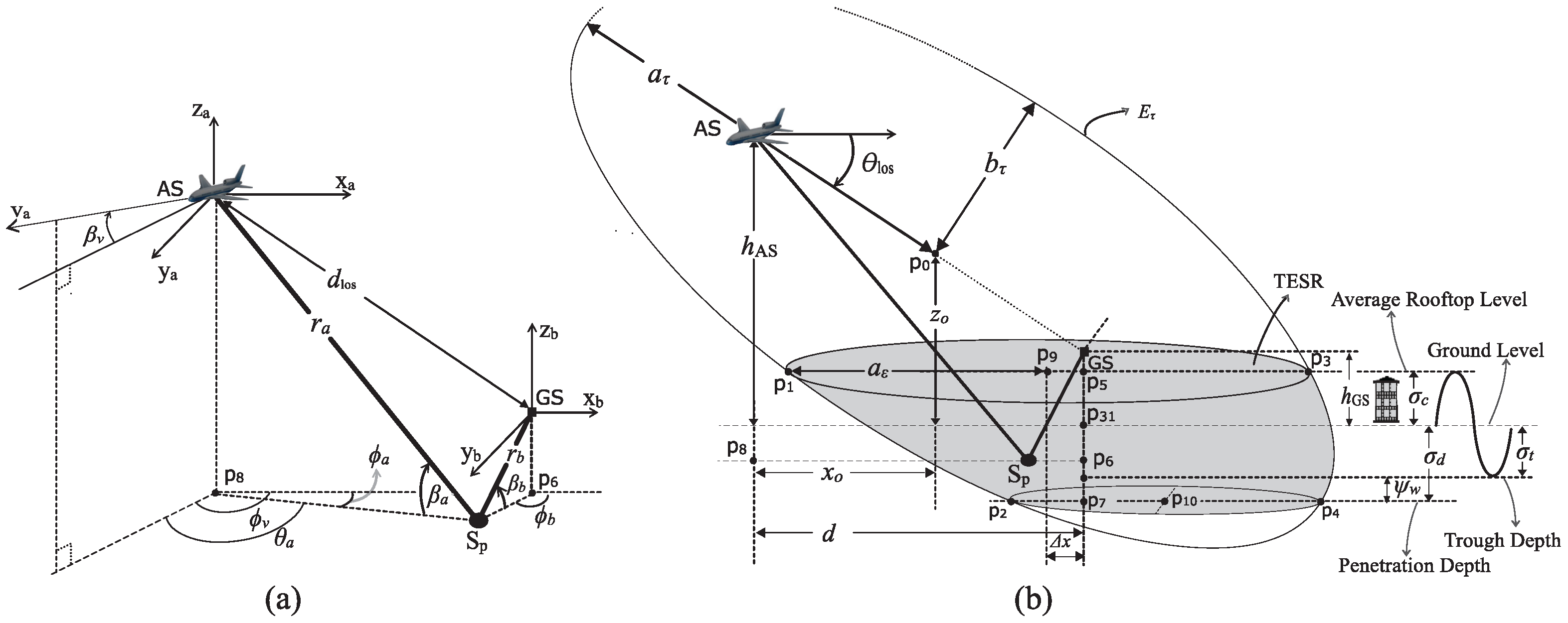
The proposed model for A2G/G2A communications is shown in Figure 1, where the AS and the GS are assumed at heights $h_{\mathrm{AS}}$ and $h_{\mathrm{GS}}$, respectively. It is assumed that AS and GS have isotropic antennas. The AS is assumed at horizontal distance d from the GS. The direct line-of-sight (LoS) distance from AS to GS is shown by $d_{\mathrm{los}}=\sqrt{d^2+{(h_{\mathrm{AS}}-h_{\mathrm{GS}})}^2},$ and the elevation angle of the LoS component with the ground plane is ${\theta }_{\mathrm{los}}=arctan\left(h_{\mathrm{AS}}-h_{\mathrm{GS}}/d\right).$ The propagation path delay associated with the longest and shortest paths is denoted by ${\tau }_{\max }$ and ${\tau }_o$, respectively. The sum of the distances from any point on the surface of an ellipsoid to each of its foci points is always the same. Using this geometric property of ellipsoids, the outer and inner boundaries of the effective scattering region can be drawn by the ellipsoids corresponding from ${\tau }_{\max }$ and ${\tau }_o$, respectively. The major and minor axes of the ellipsoid ($E_{\tau }$) can thus be obtained from the delay of the longest path (${\tau }_{\max }$), as below:

$${\displaystyle a_{\tau }=\frac{c{\tau }_{\max }}{2},}$$

(1)

$${\displaystyle c_{\tau }=b_{\tau }=(1/2)\sqrt{4a_{\tau }^2-{d_{\mathrm{los}}}^2}.}$$

(2)

The vicinity of the AS can be modelled as a scattering-free region due to the fact that the average height of an AS is usually considerably larger than the average rooftop level. The scattering region around GS is thus governed by ellipsoid ($E_{\tau }$) truncated by the planes of height equal to the average rooftop level of the surroundings or the average height of the crest and trough of sea-waves, for the cases of GS at the ground surface or the sea surface, respectively. Scattering objects are thus assumed only around the GS confined uniformly distributed within the truncated ellipsoidal-shaped scattering region (TESR) (shaded in grey in Figure 1b). A scattering point is assumed to scatter the incident signal (from any direction) in all directions with equal scattering coefficients and uniform random phases. The average vertical deviations of the crest and trough of the sea-wave from the mean level are shown with ${\sigma }_c$ and ${\sigma }_t$, respectively. For the case of communication over the ground surface, the parameter ${\sigma }_c$ will take the value based on the average rooftop height. The propagation behaviour of electromagnetic (EM) waves through the dense water medium is different from propagation in the air medium, because of water’s high permittivity and electrical conductivity. The primary limitation of EM wave propagation in dense water is the high attenuation caused by the conductivity of water [38]. The proposed model also takes the water penetration of EM waves into account for modelling the scattering region; for the low frequency band in the over-water communication scenario. The depth of penetration in meters is represented by ${\psi }_w$. This parameter may be substituted appropriately according to the frequency range and water conditions and may be substituted as zero to represent no penetration (e.g., for high frequencies). The deviation of the trough and penetration into the water together represent the depth of the scattering region, which is shown by ${\sigma }_d$ (i.e., ${\sigma }_d$ = ${\sigma }_t$ + ${\psi }_w$). For the case of A2G communication over the sea surface, the sea conditions (i.e., height of waves and roughness) are assumed to be time invariant, and scattering from the sea surface is assumed as independent of sea conditions. The angles formed in the azimuth and elevation planes with the direction of the signal corresponding to a certain scattering point ${\mathrm{S}}_{\mathrm{p}}$ at the GS are symbolized by ${\varphi }_b$ and ${\beta }_b$ and at the AS are symbolized by ${\varphi }_a$ and ${\beta }_a$, respectively. The upper face of the TESR is an ellipse whose major and minor axis is $a_{ϵ}$ and $b_{ϵ}$. ${\mathrm{p}}_9$ is the centre of this upper face ellipse. A line drawn in the x-z plane (for a value of the y coordinate taken as zero) parallel to the x-axis representing the rooftop level (or the sea-waves’ crest level) of the scattering region intersects the bounding ellipsoid $E_{\tau }$ at points ${\mathrm{p}}_1$ and ${\mathrm{p}}_3$. We can obtain the x-coordinate of the intersection points ${\mathrm{p}}_1$ and ${\mathrm{p}}_3$ by substituting the equation of the line into the equation of the bounding ellipsoid $E_{\tau }$. The major dimension $a_{ϵ}$ of the ellipse formed at the upper face of TESR along the x-axis can thus be obtained from the calculated x-coordinate of the intersection points. The expression for $a_{ϵ}$ is given below.

$$a_{ϵ}=\frac{\sqrt{-2a_{\tau }^2{b}_{\tau }^2\left(-a_{\tau }^2-b_{\tau }^2+2{\sigma }_c^2-4{\sigma }_c{z}_o+2z_o^2+(a_{\tau }^2-b_{\tau }^2)cos\left(2{\theta }_{\mathrm{los}}\right)\right)}}{a_{\tau }^2+b_{\tau }^2+(-a_{\tau }^2+b_{\tau }^2)cos\left(2{\theta }_{\mathrm{los}}\right)}.$$

(3)

The expression for minor dimension $b_{ϵ}$ obtained in the same manner is given below,

$$b_{ϵ}=b_{\tau }\sqrt{\frac{a_{\tau }^2+b_{\tau }^2-2{\sigma }_c^2+4{\sigma }_c{z}_o-2z_o^2+(-a_{\tau }^2+b_{\tau }^2)cos\left(2{\theta }_{\mathrm{los}}\right)}{a_{\tau }^2+b_{\tau }^2+(-a_{\tau }^2+b_{\tau }^2)cos\left(2{\theta }_{\mathrm{los}}\right)}}.$$

(4)

The horizontal shift of GS from the centre point is shown by $\Delta x$. The expression for $\Delta x$ can be calculated as below by using the coordinates of the GS’s position.

$$\Delta x=\frac{(a_{\tau }^2+b_{\tau }^2)x_o-(a_{\tau }^2-b_{\tau }^2)x_{o}cos\left(2{\theta }_{\mathrm{los}}\right)+(a_{\tau }^2-b_{\tau }^2)({\sigma }_c-z_o)sin\left(2{\theta }_{\mathrm{los}}\right)}{a_{\tau }^2+b_{\tau }^2+(-a_{\tau }^2+b_{\tau }^2)cos\left(2{\theta }_{\mathrm{los}}\right)},$$

(5)

The shift of bounding ellipsoid $E_{\tau }$ in the x- and z-axis is represented by the parameters $x_o$ and $z_o$, respectively, with respect to the base of AS, which can be obtained as,

$$x_o=\frac{d_{\mathrm{los}}}{2}cos{\theta }_{\mathrm{los}},$$

(6)

$$z_o=h_{\mathrm{AS}}-\frac{d_{\mathrm{los}}}{2}sin{\theta }_{\mathrm{los}}.$$

(7)

The angles ${\beta }_{\min }$ and ${\beta }_{\max }$ are angular limits of the elevation angle observed at AS, which can be defined as,

$${\beta }_{\min }=arctan\left(\frac{h_{\mathrm{AS}}-{\sigma }_c}{d-\Delta x+a_{ϵ}}\right)$$

(8)

$${\beta }_{\max }=\left\{\begin{array}{cc}arctan\left(\frac{h_{\mathrm{AS}}-{\sigma }_c}{d-\Delta x-a_{ϵ}}\right)\hfill & ,d>a_{ϵ}+\Delta x.\hfill \\ \frac{\pi }{2}\hfill & ,d\le a_{ϵ}+\Delta x.\hfill \end{array}\right.$$

(9)

The angles ${\varphi }_{\min }$ and ${\varphi }_{\max }$ represent the lower and upper angular limit of the azimuthal angle observed at AS, which can be defined as,

$${\displaystyle \left.\begin{array}{c}{\varphi }_{\max }^{+}\hfill \\ {\varphi }_{\min }^{-}\hfill \end{array}\right\}=\left\{\begin{array}{cc}\pm arctan\left(\mp \frac{b_{ϵ}}{\sqrt{-a_{ϵ}^2+{(d-\Delta x)}^2}}\right)\hfill & ,d>a_{ϵ}+\Delta x.\hfill \\ \\ \pm \pi \hfill & ,d<a_{ϵ}+\Delta x.\hfill \end{array}\right.}$$

(10)

A scattering object is assumed (defined) to be a lossless re-radiating element, which redirects (reflects) a part of the incident wave’s power directly towards the receiver. The distance of a certain scattering point ${\mathrm{S}}_{\mathrm{p}}$ from AS and GS is $r_a$ and $r_b$, respectively. The total length of a signal from GS to AS (via a single bounce) can thus be given as,

$$l=r_b+r_a.$$

(11)

$r_b$ is the distance of a scatterer from GS and can be written in simplified form as,

$${\displaystyle r_b=\sqrt{d^2+r_a^2{cos}^2{\beta }_a-2r_{a}dcos{\beta }_{a}cos{\varphi }_a+(h_{\mathrm{AS}}-h_{\mathrm{GS}}+r_a{sin}^2{\beta }_a)}.}$$

(12)

Substituting the value of $r_b$ in (11) and solving for $r_a$, the equation for $r_a$ as a function of path delay and angles seen on AS can be rearranged as,

$${\displaystyle r_a=\frac{l^2-d_{\mathrm{LoS}}^2}{2(l-dcos{\beta }_{a}cos{\varphi }_a-(h_{\mathrm{AS}}-h_{\mathrm{GS}})sin{\beta }_a)}.}$$

(13)

V is the volume of TESR, which is an important parameter for the case of uniform scatterers, which can be calculated by the same approach as given in [21] for a similar geometry. The solution for V can thus be expressed in compact form as given below,

$$\begin{array}{c}{\displaystyle V=\frac{1}{3\sqrt{{(a_{\tau }^2+b_{\tau }^2+(-a_{\tau }^2+b_{\tau }^2)cos\left(2{\theta }_{\mathrm{los}}\right))}^3}}\times \{\sqrt{2}{a}_{\tau }{b}_{\tau }^2\pi ({\sigma }_c+{\sigma }_t+{\psi }_w)}\hfill \\ {\displaystyle (3a_{\tau }^2+3b_{\tau }^2-2{({\sigma }_c+{\sigma }_t+{\psi }_w)}^2+6({\sigma }_c+{\sigma }_t+{\psi }_w)(h_{\mathrm{AS}}-\frac{d_{\mathrm{los}}}{2}sin{\theta }_{\mathrm{los}})}\hfill \\ {\displaystyle -6{(h_{\mathrm{AS}}-\frac{d_{\mathrm{los}}}{2}sin{\theta }_{\mathrm{los}})}^2+3(-a_{\tau }^2+b_{\tau }^2)cos\left(2{\theta }_{\mathrm{los}}\right))\}.}\hfill \end{array}$$

(14)

3. PDF of the Normalized Doppler Spectrum

The angles ${\varphi }_v$ and ${\beta }_v$ are azimuth and elevation angles along the direction of the motion of AS, respectively. The azimuth and elevation angle of the motion of AS with a certain multipath signal are represented by ${\theta }_a={\varphi }_v-{\varphi }_a$ and ${\alpha }_a={\beta }_v-{\beta }_a$, respectively. The velocity of AS is denoted by $v_a$. The Doppler shift of a certain multipath can be obtained as,

$${\displaystyle f_{DS}=f_{m}cos{\theta }_{a}cos{\alpha }_a.}$$

(15)

However, the maximum shift in the Doppler spectrum can be given as $f_m=(v_a/c)f_c$, where c is the velocity of light and $f_c$ is the carrier frequency. The normalized Doppler spectrum [26,27,39] can be expressed as follows,

$${\displaystyle \gamma =f_{DS}/f_m=cos{\theta }_{a}cos{\alpha }_a.}$$

(16)

The azimuth angle ${\varphi }_a$ can be expressed as a function of the direction of motion, elevation AoA and Doppler shift, which is as below,

$${\displaystyle {\varphi }_a={\varphi }_v-{cos}^{-1}\left(\gamma /cos({\beta }_v-{\beta }_a)\right)}$$

(17)

The joint density function of azimuth AoA, elevation AoA and propagation path distance $p(l,{\varphi }_a,{\beta }_a)$ can be obtained by transforming the density function $p(r_a,{\varphi }_a,{\beta }_a)$ using the relationship given in (13) from the following equation.

$${\displaystyle p(l,{\varphi }_a,{\beta }_a)=\frac{p(r_a,{\varphi }_a,{\beta }_a)}{\left|J\right(l,{\varphi }_a,{\beta }_a\left)\right|}.}$$

(18)

The joint density function given in (18), $p(r_a,{\varphi }_a,{\beta }_a)$, can be expressed as, given in [21],

$${\displaystyle p\left(r_a,{\varphi }_a,{\beta }_a\right)=r_a^{2}cos{\beta }_{a}f(x,y,z).}$$

(19)

where $f(x,y,z)$ represents the spatial distribution of scatterers. This density can be written as $f(x,y,z)=1/V$ for a uniform distribution of scatterers. The Jacobian transformation given in (18), $J(l,{\varphi }_a,{\beta }_a)$, can be derived as,

$${\displaystyle J(l,{\varphi }_a,{\beta }_a)={\left|\frac{\partial r_a}{\partial l}\right|}^{-1}=\frac{2{(l-dcos{\beta }_{a}cos{\varphi }_a+(-h_{\mathrm{AS}}+h_{\mathrm{GS}})sin{\beta }_a)}^2}{l^2+d_{\mathrm{LoS}}^2-2l(dcos{\beta }_{a}cos{\varphi }_a+(h_{\mathrm{AS}}-h_{\mathrm{GS}})sin{\beta }_a)}.}$$

(20)

Substituting (19) and (20) in (18), the simplified solution for $p(l,{\varphi }_a,{\beta }_a)$ can be re-written as,

$${\displaystyle p(l,{\varphi }_a,{\beta }_a)=\frac{d_{\mathrm{LoS}}^2+l^2-2l(dcos{\beta }_{a}cos{\varphi }_a+(h_{\mathrm{AS}}-h_{\mathrm{GS}})sin{\beta }_a)}{8Vsec{\beta }_a{(l-dcos{\beta }_{a}cos{\varphi }_a+(-h_{\mathrm{AS}}+h_{\mathrm{GS}})sin{\beta }_a)}^4}{(d_{\mathrm{LoS}}^2-l^2)}^2.}$$

(21)

The power received from a certain multipath p can be obtained by using the path loss model given in [39] as,

$${\displaystyle p_r\left(l_p\right)=p_o{\left(\frac{l_p}{d_{\mathrm{LoS}}}\right)}^{-n},}$$

(22)

where $d_{\mathrm{LoS}}$ is the length of LoS from GS to AS, $p_o$ is the power received corresponding to the LoS component, n is the path loss exponent and $l_p$ is the length of the p-th multipath. By re-arranging this relation for $l_p$, we get:

$$l_p=d_{\mathrm{LoS}}{\left(\frac{p_r}{p_o}\right)}^{-\frac{1}{n}}.$$

(23)

The joint density function $p(p_r,{\varphi }_a,{\beta }_a)$ can be obtained by transforming the density function $p(l,{\varphi }_a,{\beta }_a)$ using the relationship given in (23),

$${\displaystyle p(p_r,{\varphi }_a,{\beta }_a)={\left.\frac{p(l_p,{\varphi }_a,{\beta }_a)}{\left|J\right(l_p,{\varphi }_a,{\beta }_a\left)\right|}\right|}_{l_p=d_{\mathrm{LoS}}{\left(\frac{p_r}{p_o}\right)}^{-\frac{1}{n}}}.}$$

(24)

The Jacobian transformation shown in (24) can be derived as:

$${\displaystyle J(l_p,{\varphi }_a,{\beta }_a)={\left|\frac{\partial l_p}{\partial p_r}\right|}^{-1}=\frac{-n{p}_o}{d_{\mathrm{LoS}}}{\left(\frac{p_r}{p_o}\right)}^{\frac{n+1}{n}}.}$$

(25)

Substituting (21) and (25) in (24) and considering the following assumptions, $k={\left(p_r/p_o\right)}^{\frac{1}{n}},h_e=(h_{\mathrm{AS}}-h_{\mathrm{GS}}),$ the joint density function $p(p_r,{\varphi }_a,{\beta }_a)$ can be given in simplified form as below,

$$\begin{array}{c}{\displaystyle p(p_r,{\varphi }_a,{\beta }_a)=\frac{1}{(8Vsec{\beta }_{a}n{p}_r){\left(-d_{\mathrm{LoS}}+dkcos{\beta }_{a}cos{\varphi }_a+h_{e}ksin{\beta }_a\right)}^4}\times }\hfill \\ \left\{-d_{\mathrm{LoS}}^6{k}^{-3}{\left(-1+k^2\right)}^2\left(d_{\mathrm{LoS}}\left(1+k^2\right)-2dkcos{\beta }_{a}cos{\varphi }_a-2h_{e}ksin{\beta }_a\right)\right\}\hfill \end{array}$$

(26)

The secant function represents $sec(.)=1/cos(.)$. The joint density function $p(p_r,\gamma ,{\beta }_a)$, can be obtained by transforming the density function $p(p_r,{\varphi }_a,{\beta }_a)$ using the relationship given in (17),

$${\displaystyle p(p_r,\gamma ,{\beta }_a)={\left.\frac{p(p_r,{\varphi }_a,{\beta }_a)}{\left|J\right(p_r,{\varphi }_a,{\beta }_a\left)\right|}\right|}_{{\varphi }_a={\varphi }_v-{cos}^{-1}\left(\frac{\gamma }{cos({\beta }_v-{\beta }_a)}\right).}}$$

(27)

The Jacobian transformation shown in (27) can be derived as,

$${\displaystyle J(p_r,{\varphi }_a,{\beta }_a)={\left|\frac{\partial {\varphi }_a}{\partial \gamma }\right|}^{-1}=\sqrt{{cos}^2({\beta }_a-{\beta }_v)-{\gamma }^2}.}$$

(28)

Substituting (26) and (28) in (27), the joint density function in (27) can be given in simplified form as below.

$$\begin{array}{c}{\displaystyle p(p_r,\gamma ,{\beta }_a)=\{\left(\frac{-d_{\mathrm{LoS}}^6{\left(-1+k^2\right)}^2}{8V{k}^{3}sec{\beta }_{a}cos({\beta }_a-{\beta }_v)n{p}_r\sqrt{(}1-{\gamma }^2{sec}^2({\beta }_a-{\beta }_v))}\right)}\hfill \\ \times {\left(-d_{\mathrm{LoS}}+dkcos{\beta }_{a}cos({\varphi }_v-arccos(\gamma sec({\beta }_a-{\beta }_v)))+h_{e}ksin{\beta }_a\right)}^{-4}\hfill \\ {\displaystyle \times (d_{\mathrm{LoS}}\left(1+k^2\right)-(2dkcos{\beta }_{a}cos({\varphi }_v-arccos(\gamma sec({\beta }_a-{\beta }_v)))}\hfill \\ {\displaystyle -2h_{e}ksin{\beta }_a\left)\right)\}.}\hfill \end{array}$$

(29)

The joint PDF for the Doppler and power can thus be derived after integrating (29) over ${\beta }_a$ for its appropriate range.

$$\begin{array}{c}{\displaystyle p(p_r,\gamma )={\int }_{{\beta }_l\left(\gamma \right)}^{{\beta }_u\left(\gamma \right)}p(p_r,\gamma ,{\beta }_a)\mathrm{d}{\beta }_a.}\hfill \end{array}$$

(30)

It is obvious from (16), that $|cos{\theta }_a\le 1|$; we may have $\left|\gamma \right|\le cos\left({\beta }_a\right).$ Therefore, here, ${\beta }_u\left(\gamma \right)$ and ${\beta }_l\left(\gamma \right)$ can be defined by the same approach used in [40].

$${\displaystyle {\beta }_u\left(\gamma \right)=\left\{\begin{array}{cc}{\beta }_{\max }\hfill & ,0\le \left|\gamma \right|\le cos{\beta }_{\max },\hfill \\ arccos\left(\right|\gamma \left|\right)\hfill & ,cos{\beta }_{\max }\le \left|\gamma \right|\le 1.\hfill \end{array}\right.}$$

(31)

$${\displaystyle {\beta }_l\left(\gamma \right)=\left\{\begin{array}{cc}-{\beta }_{\min }\hfill & ,0\le \left|\gamma \right|\le cos{\beta }_{\min },\hfill \\ -arccos\left(\right|\gamma \left|\right)\hfill & ,cos{\beta }_{\min }\le \left|\gamma \right|\le 1.\hfill \end{array}\right.}$$

(32)

The marginal PDF for the Doppler shift for the proposed model can thus be derived by integrating (30) over $p_r$,

$$\begin{array}{c}{\displaystyle p\left(\gamma \right)={\int }_{p_l}^{p_u}p(p_r,\gamma )\mathrm{d}{p}_r.}\hfill \end{array}$$

(33)

$p_u$ and $p_l$ are the upper and lower limits of the received power. The power received from the shortest propagation path is the maximum power. The shortest path in this model is $d_{\mathrm{LoS}}$; so from (22), it is evident that $p_u=p_o$. For a particular azimuth and elevation angle, the multipath component received from the boundary of the scattering region is the longest propagation path. The power received from the longest propagation path is the lowest power received. We know that the longest delay for the reflected wave is ${\tau }_{\max }$, which is assumed to be a known value on the receiver. Therefore, the lower limit for the received power can thus be obtained as:

$${\displaystyle p_l=p_o{\left(\frac{{\tau }_{\max }}{c{d}_{\mathrm{LoS}}}\right)}^{-n}.}$$

(34)

The definition of the cumulative distribution function (CDF) of the Doppler shift is:

$${\displaystyle F\left(\gamma \right)={\int }_{-1}^{\gamma }p\left(\Gamma \right)\mathrm{d}\Gamma .}$$

(35)

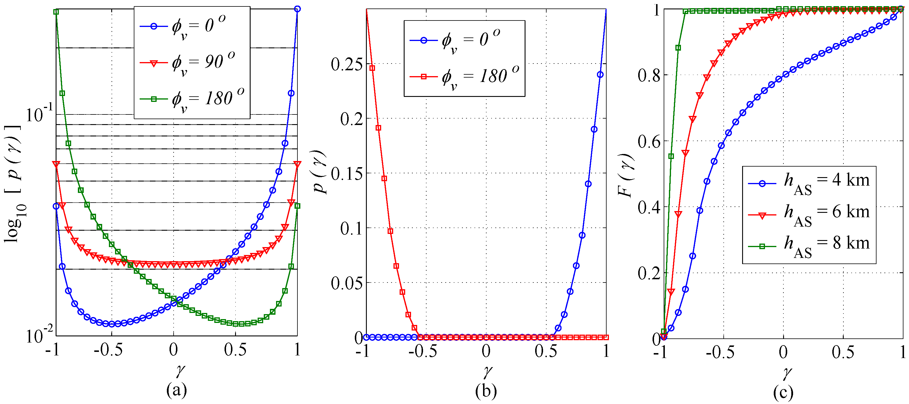
The results for the marginal PDF of the Doppler spectrum are obtained by numerically integrating the trivariate density function in (29) over elevation AoA and power for appropriate limits. These results are obtained in relation to the direction of motion in the azimuth and the elevation plane. The impact of the important parameters of the proposed channel model, such as the height of AS and the longest path’s delay, is also studied on the Doppler spectrum. The scatterers are assumed as uniformly distributed for obtaining these results. The effect of the direction of the motion of AS in the azimuth plane (${\varphi }_v$) on the marginal PDF of the Doppler spectrum is shown in Figure 2a,b. When the geometric scenario is such that the projection of AS on the x-y plane lies within the scattering region, the probability of the arrival of multipath waves at AS is the same from all of the directions in the azimuth plane. It can be seen that for ${\varphi }_v={90}^{\circ }$, the PDF is observed as U-shaped and symmetric around $\gamma =0$. This is due to the fact that multipath components contributing to the maximum and minimum Doppler shift are present in an equal amount. For ${\varphi }_v=0^{\circ }$ and ${\varphi }_v={180}^{\circ }$, the PDF is seen tilted towards the lower and higher frequencies, respectively. Moreover, when the image of AS on the x-y plane is away from the scattering region and the elevation of AS is set as $h_{\mathrm{AS}}$ = 7 km, this can be an en-route scenario; the spatial distribution of the scatterers is non-isotropic. This leads to the selection of only a part of the band from the whole U-shaped PDF of the Doppler shift depending on the direction of the AS’s mobility, which is evident in Figure 2b. The effect of the change in the elevation of AS on the CDF of the Doppler spectrum is shown in Figure 2c, plotted for the different values of $h_{\mathrm{AS}}$. It can be observed that with an increase in the height of AS, the angular spread decreases, which further leads to an increase in the slope of CDF.

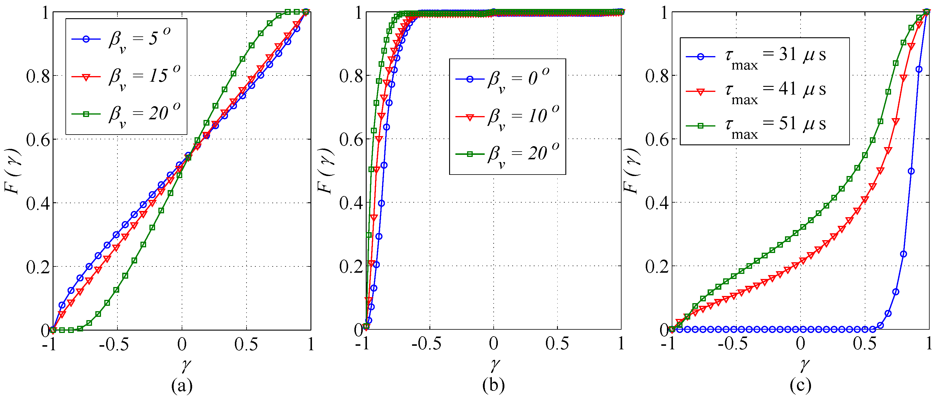
The effect of the direction of the motion of AS in the elevation plane (${\beta }_v$) on the CDF of the Doppler spectrum is shown in Figure 3a,b. When the projection of AS on the x-y plane lies inside the scattering region, the CDFs are symmetric around $\gamma =0$. It can be observed that with an increase in the angle for the elevational direction of motion, the slope of CDF slowly decreases up to $\gamma =0$ and then increases slowly, and CDF approaches one when γ approaches one.

When distance between nodes is increased, and the shadow of AS on the x-y plane is outside the scattering region; the spread in angular data observed at AS decreases to a smaller number from $2\pi$. Therefore, CDFs are approaching one very quickly. The increase in delay span defines an increase in the horizontal dimensions of TESR. This effect of increasing the delays of the longest paths on the Doppler spectrum is demonstrated in Figure 3c. It can be observed that for large values of the delays of the longest paths, the dimension of the TESR is large enough to have the projection of AS on the x-y plane inside the scattering region; therefore, the signals are received from all around, so the CDFs of the Doppler shift are almost symmetric around $\gamma =0$. 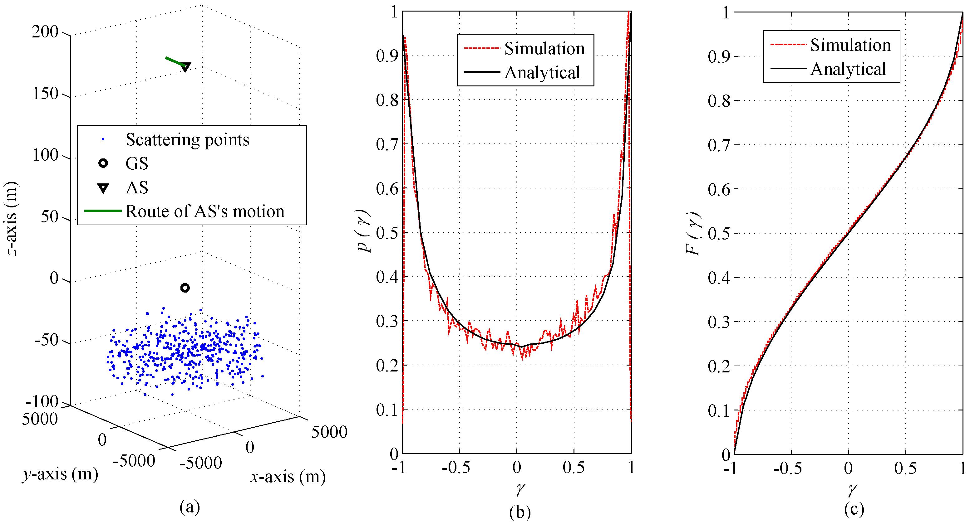The obtained analytical results are also validated through the comparison with the performed simulation results. The computer simulations are performed by adopting the approach presented in detail in [41]. The scatterers are generated in the defined TESR, as shown in Figure 4a. The positions of AS and GS are also shown in Figure 4a. The direction of the motion of AS in the azimuth plane is taken as ${\varphi }_v={90}^{\circ }$. The heights of AS and GS are assumed such that AS is close to the ground level. Using the simulation setup, the simulated results for the PDF of the Doppler spectrum are compared to the proposed analytical results shown in Figure 4b, where PDF is U-shaped because the multipath components contributing in the positive and negative Doppler are in equal amounts. The simulated results for the CDF of the Doppler spectrum are compared to the proposed analytical results in Figure 4c. For ${10}^3$ uniformly distributed scattering points and averaging over 2000 Monte Carlo runs, a good match is observed between simulation and analytical results.

4. Shape Factors

The SFs proposed in [28] are the favourable parameters for the quantification of spatial spread. The joint PDF of AoA, the marginal PDF of azimuth AoA and the marginal PDF of elevation AoA can be represented by $p({\varphi }_m,{\beta }_m)$, $p\left({\varphi }_m\right)$, $p\left({\beta }_m\right)$, where the subscript m may be replaced by a or b for the statistics of the AS and GS sides, respectively. The joint and marginal PDFs of AoA for such A2G/G2A scenarios w.r.t. the azimuth and elevation angles observed from both ends of the link are derived in [21]. The methodology used for computing the SFs is consistent with the methods proposed in [28,29]. Fourier coefficients or trigonometric moments are used for analysing the PDF of AoA. These two methods are similar in definition; however, the approach given in [29] is applicable for discrete measurements of angular data.

The n-th complex trigonometric moment of any angular distribution is ${\overline{R}}_n$. For example, for $p\left(\phi \right)$ (i.e., where φ may be ${\varphi }_m$ or ${\beta }_m$ for the azimuthal and elevational AoA), whose total power is equal to $P_o={\int }_0^{2\pi }p\left(\phi \right)\mathrm{d}\phi$, ${\overline{R}}_n$ is defined as,

$${\overline{R}}_n={\overline{C}}_n+j{\overline{S}}_n,$$

(36)

where,

$${\overline{C}}_n=\frac{1}{P_o}{\int }_0^{2\pi }p\left(\phi \right)cos\left(n\phi \right)\mathrm{d}\phi$$

(37)

and,

$${\overline{S}}_n=\frac{1}{P_o}{\int }_0^{2\pi }p\left(\phi \right)sin\left(n\phi \right)\mathrm{d}\phi .$$

(38)

In the case of discrete data, the definition for trigonometric moments can be modified. Only first and second moments are used in the characterization of the SFs. $|{\overline{R}}_1|$ is the magnitude of the first trigonometric moment. It can take values between zero and one. A close to zero value means the receiver is receiving signals from a wider range of angles, and close to one means a small angular width of AoA. The SF angular spread, ${\mathsf{\Lambda }}_{{\phi }_m}$, is given as below,

$${\mathsf{\Lambda }}_{{\phi }_m}=\sqrt{1-|{\overline{R}}_1{|}^2}.$$

(39)

The other two SFs, angular constriction ${\gamma }_{{\phi }_m}$ and orientation parameter ${\phi }_m^{MF}$, are defined by Durgin et al. in [28]. ${\gamma }_{{\phi }_m}$ gives the concentration of the multipath about two directions, and ${\phi }_m^{MF}$ provides the direction of maximum fading. Their relation with trigonometric moments is given below,

$${\gamma }_{{\phi }_m}=\frac{|{\overline{R}}_2-{\overline{R}}_1^2|}{1-|{\overline{R}}_1{|}^2},$$

(40)

and:

$${\phi }_m^{MF}=\frac{1}{2}\mathrm{phase}\{{\overline{R}}_2-{\overline{R}}_1^2\}.$$

(41)

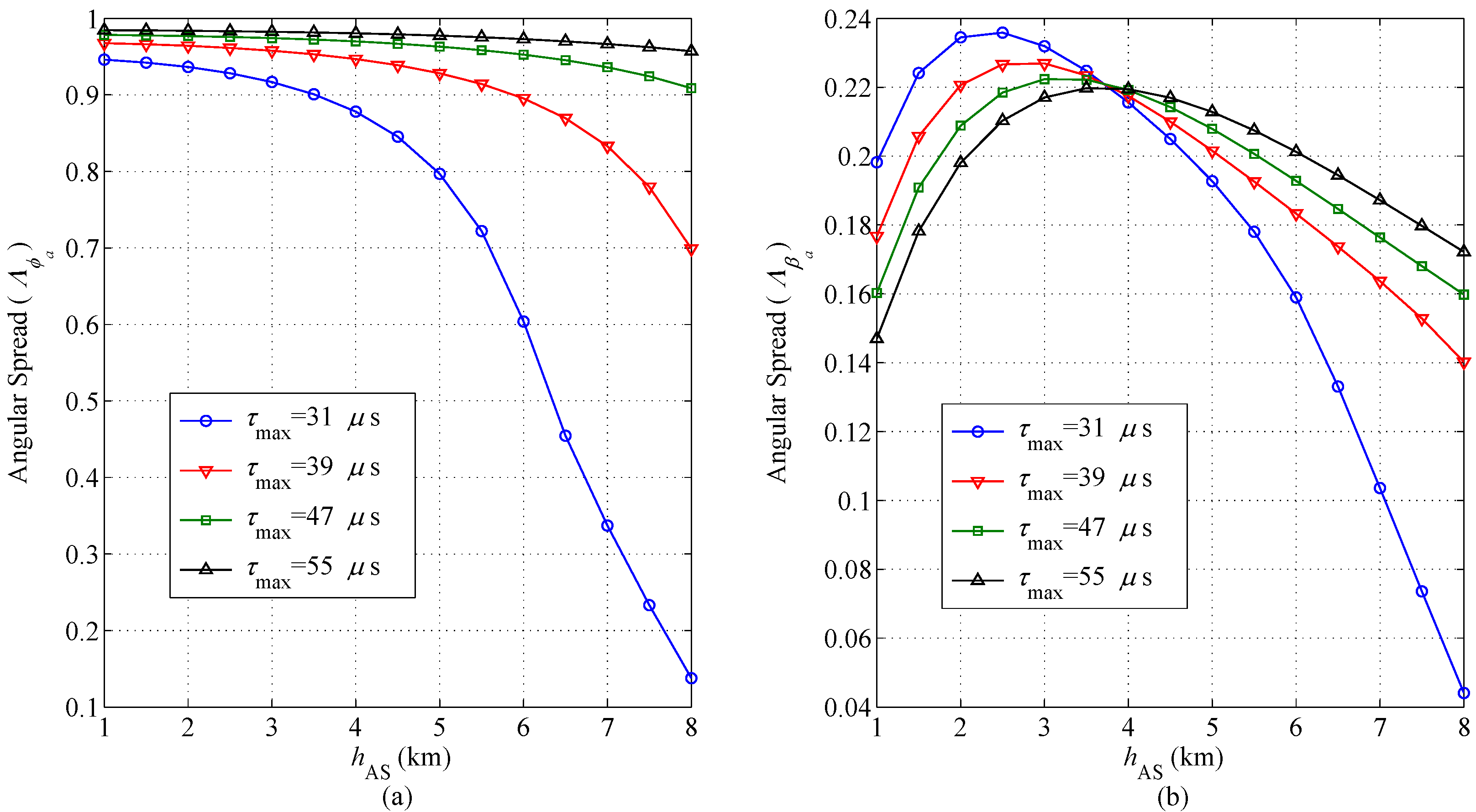
A thorough analysis on the results of the SFs for the A2G/G2A communication channel is presented. The SF angular spread ${\mathsf{\Lambda }}_{{\phi }_m}$ gives the measurement of the concentration of multipaths around a single direction by using the range zero to one. The azimuthal and elevational angular spread observed from AS with respect to the height of AS for different delays of the longest propagation path is shown in Figure 5a,b, respectively. The azimuthal angular spread decreases with an increase in the height of AS. However, the rate of decrease increases rapidly with respect to the increase in the height of AS by reducing the ${\tau }_{\max }$. The elevational angular spread observed from AS increases gradually with the increase in height of AS up to the height when the projection of AS on the x-y plane lies within the scattering region, and it decreases with the further increase in the height of AS. Moreover, the elevational angular spread shows a converse trend with respect to ${\tau }_{\max }$. The elevational angular spread with an increase in ${\tau }_{\max }$ decreases up to a certain height of AS: whereas, with the further increase in the height of AS, it increases.

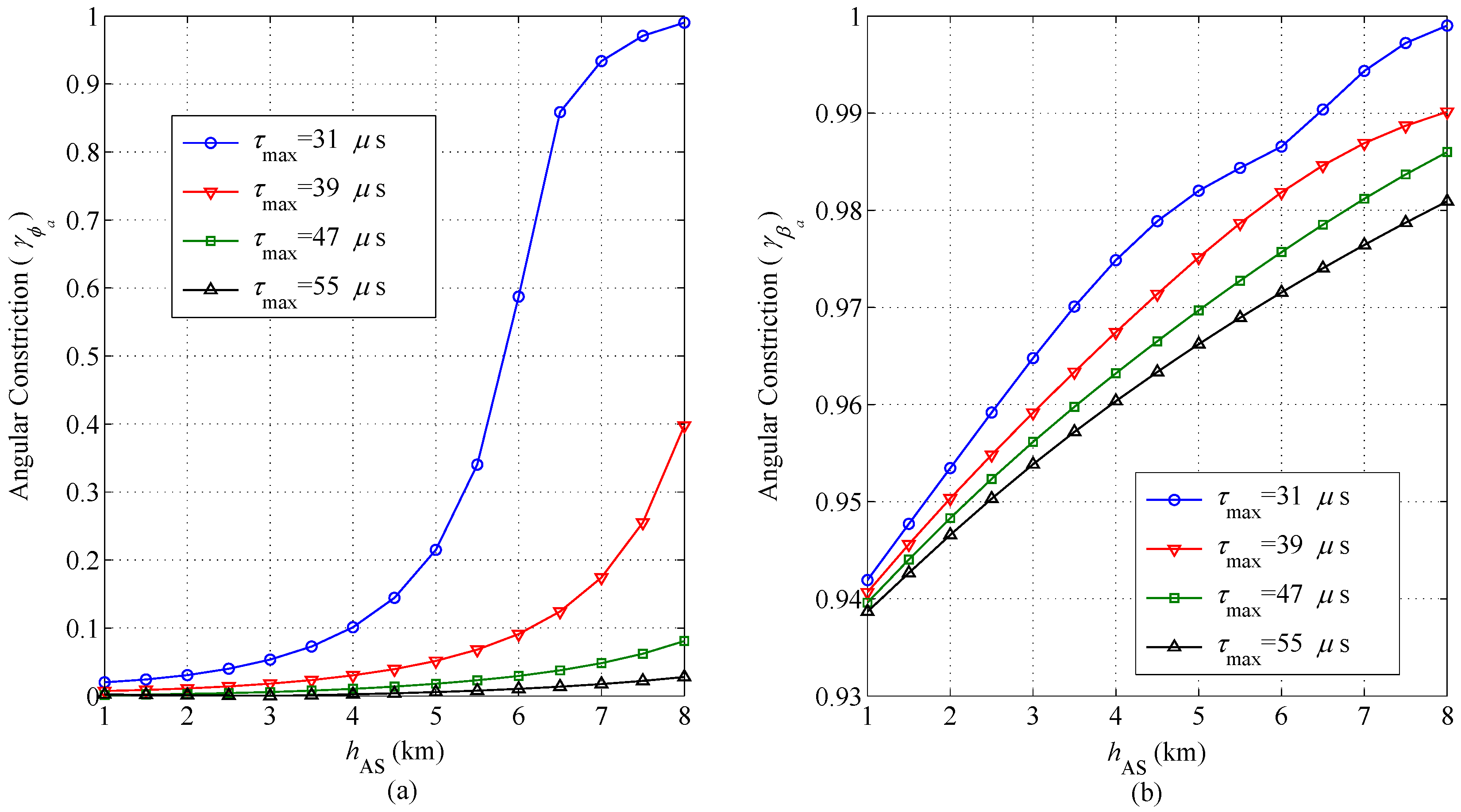
The SF angular constriction ${\gamma }_{{\phi }_m}$ gives a measure of the concentration of multipaths around two directions. The value for ${\gamma }_{{\phi }_m}$ ranges from zero to one, with one denoting the arrival of exactly two multipath components from different directions and zero denoting no clear bias in two arrival directions [28]. The angular constriction for the azimuth and elevation angles observed from AS with respect to the height of AS is plotted in Figure 6a,b, respectively.

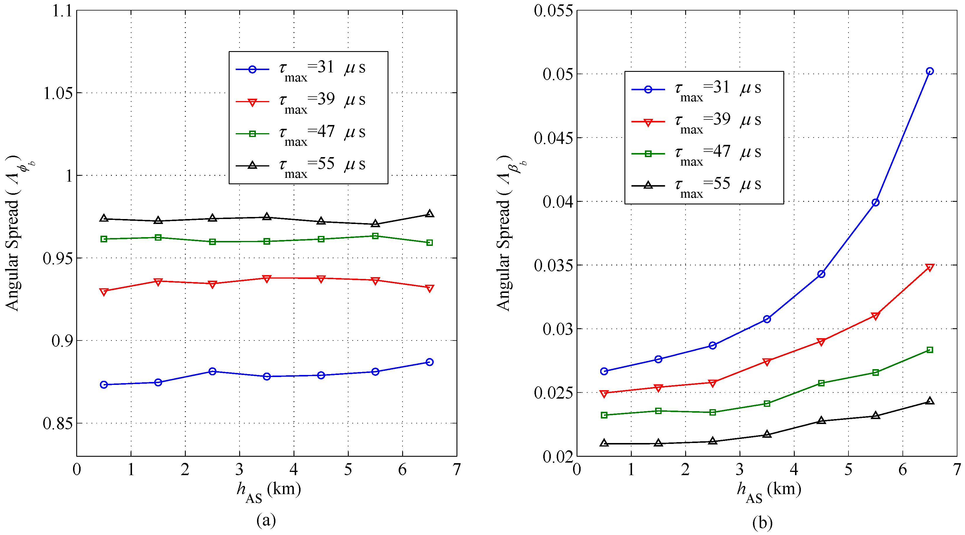
The angular constriction w.r.t. the azimuth angles increases with the increase in the height of AS; however, the rate of increase decreases with the increase in ${\tau }_{\max }$. The angular constriction w.r.t. the elevation angles gradually increases with the increase in the height of AS. Moreover, with the increase in ${\tau }_{\max }$, it decreases. The azimuthal and elevational angular spread observed from GS with respect to the height of AS for different values of ${\tau }_{\max }$ is shown in Figure 7a,b, respectively. The azimuthal angular spread is observed to be constant (approximately) with respect to the increase in height of AS; however, it increases with the increase in ${\tau }_{\max }$. An exponential increase is observed in the angular spread in the elevation plane seen at GS with the increase in the height of AS. Furthermore, the rate of the increase in the angular spread decreases with the increase in ${\tau }_{\max }$. 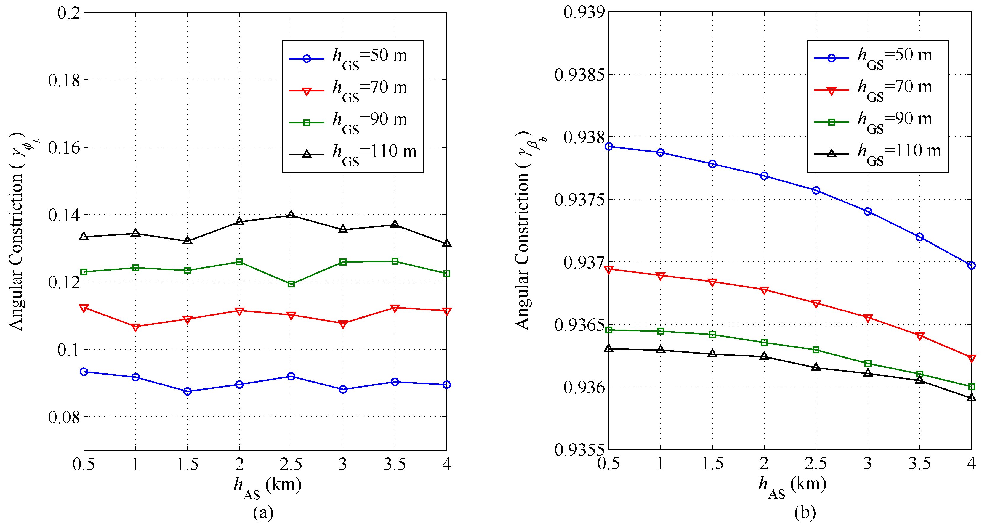The angular constriction for the azimuth and elevation angles for different values of the height of GS observed from GS with respect to the height of AS is plotted in Figure 8a,b, respectively. The angular constriction remains almost constant with respect to the azimuth angles with the increase in the height of AS as long as AS lies inside the scattering region; however, it increases with the increase in $h_{\mathrm{GS}}$. The angular constriction with the elevation angles has a gradual decrease with the increase in the height of AS. However, conversely with the azimuthal side, it decreases with the increase in $h_{\mathrm{GS}}$.

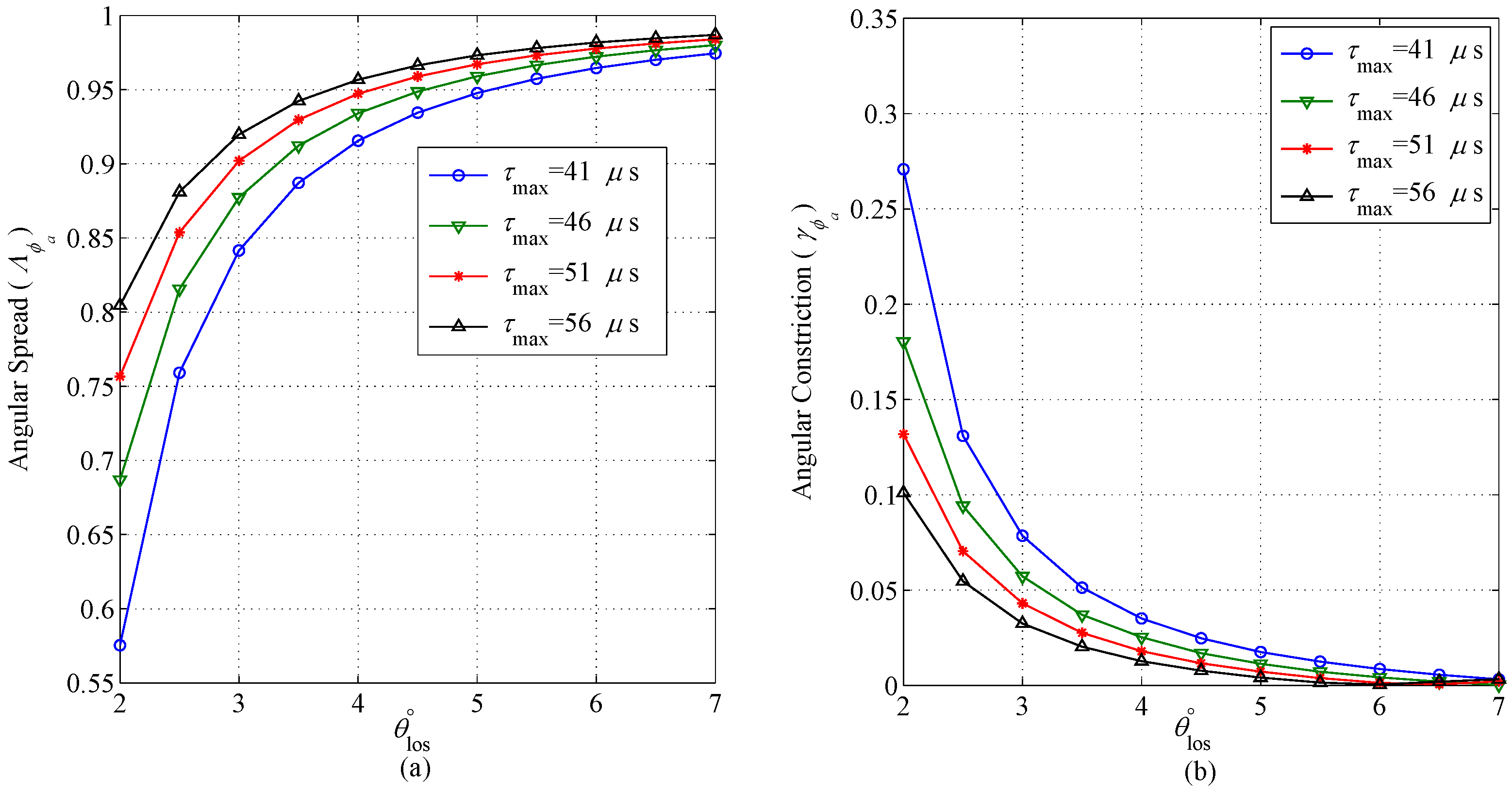
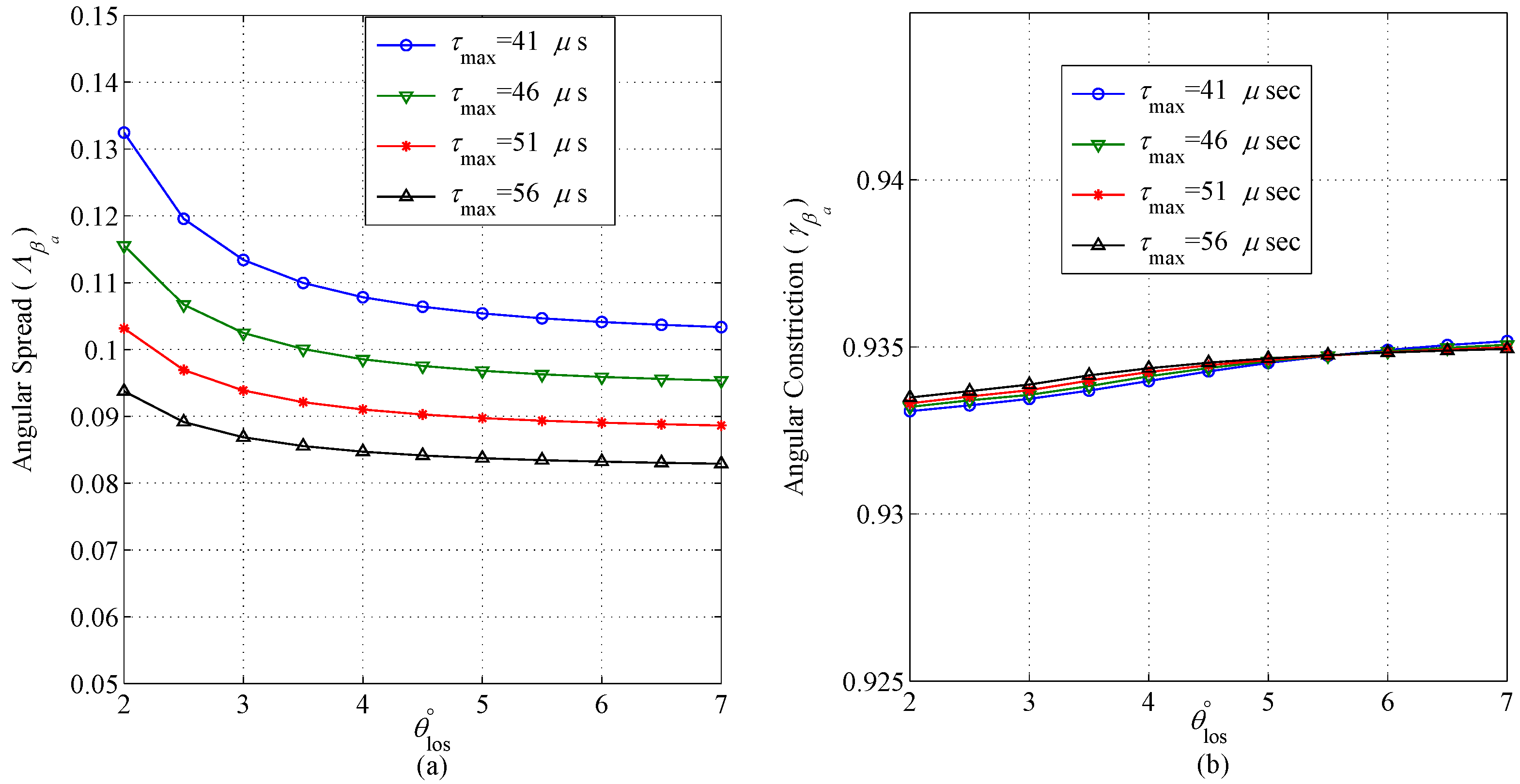
The azimuthal and elevational angular spread observed at the AS side of the link with respect to the variations in the elevational LoS angle ${\theta }_{\mathrm{los}}$ and the delay of the longest propagation path ${\tau }_{\max }$ is shown in Figure 9a and Figure 10a, respectively. When AS moves away from GS, the elevation LoS angle reduces. Subsequently, the azimuthal angular spread increases, and the elevational angular spread reduces. This is true for all of the values of ${\tau }_{\max }$; however, the rate of change is different for different values of ${\tau }_{\max }$. The concentration of energy about exactly two physical directions (angular constriction) observed at the AS side independently in both the azimuth and elevation planes is shown in Figure 9b and Figure 10b, respectively. In the azimuth plane, the distribution of energy has a higher bias towards two physical angles for lower values of both the elevation LoS angle and delay span. For elevation LoS angles, ${\theta }_{\mathrm{los}}>6^{\circ }$, there is almost no bias in the distribution of energy towards two azimuthal angles. On the other hand, the change in elevation LoS angle and delay span has a very marginal impact on the elevational angular constriction; see Figure 10b. This is because the impact of these two parameters on changing the dimensions of the scattering region along the vertical axis is very marginal; rather, the dimensions of the scattering region along vertical axis depend on the vertical size of the scattering structures (buildings, etc.) in the vicinity of GS. The delay of the longest path and the height of AS does not impact the symmetry of the scattering region with respect to the observing end in the azimuth plane; therefore, the azimuthal direction of maximum fading is observed as a constant value for all of the values of ${\tau }_{\max }$ and $h_{\mathrm{AS}}$; i.e., ${\varphi }_a^{MF}=\pm {90}^{\circ }$ and ${\varphi }_b^{MF}=0^{\circ }$.

5. Second Order Fading Statistics

SFs can further be used to study the second order fading statistics, like LCR, AFD, auto-covariance and the coherence distance of the propagation channel. These statistics are defined in terms of angular spread, angular constriction and the direction of maximum fading, as in [28,35]. Azimuthal SFs are used in the analysis of the second order fading statistics. The LCR, ${\mathit{N}}_{\mathit{R}}$, quantifies how often a threshold is crossed by a fading and is defined as,

$$N_R=\sqrt{2\pi }{\mathsf{\Lambda }}_{{\varphi }_m}{f}_m\rho \sqrt{1+{\gamma }_{{\varphi }_m}cos\left(2({\varphi }_v-{\varphi }_m^{MF})\right)\exp (-{\rho }^2)},$$

(42)

where ρ is the normalised threshold level.

The AFD, $\overline{\tau }$, quantifies the time spent by a signal below the threshold level and can be defined by the relation given below,

$$\overline{\tau }=\frac{(\exp (-{\rho }^2)-1)}{\sqrt{2\pi }{\mathsf{\Lambda }}_{{\varphi }_m}{f}_m\rho \sqrt{1+{\gamma }_{{\varphi }_m}cos\left(2({\varphi }_v-{\varphi }_m^{MF})\right)}}.$$

(43)

Auto-covariance is another important statistic, which determines the correlation of the received voltage envelope as a function of the change in the receiver position and is useful for studies in spatial diversity [28,42]. An expression of auto-covariance based on SFs is given in [43], which can be approximated as below,

$$p(r,{\varphi }_v)\approx \exp \left[-23{\mathsf{\Lambda }}_{{\varphi }_m}^2\left(1+{\gamma }_{{\varphi }_m}cos\left(2({\varphi }_v-{\varphi }_m^{MF})\right)\right){\left(\frac{r}{\lambda }\right)}^2\right].$$

(44)

This equation provides the envelop correlation between two points separated by distance $\mathit{r}$. The coherence distance, ${\mathit{D}}_{\mathit{c}}$, is the separation in space over which channel response is unchanged. It is important for spatial diversity in the design of wireless receivers. The coherence distance can be defined as,

$$D_c\approx \frac{\lambda \sqrt{ln\left(2\right)}}{{\mathsf{\Lambda }}_{{\varphi }_m}\sqrt{23\left(1+{\gamma }_{{\varphi }_m}cos\left(2({\varphi }_v-{\varphi }_m^{MF})\right)\right)}}.$$

(45)

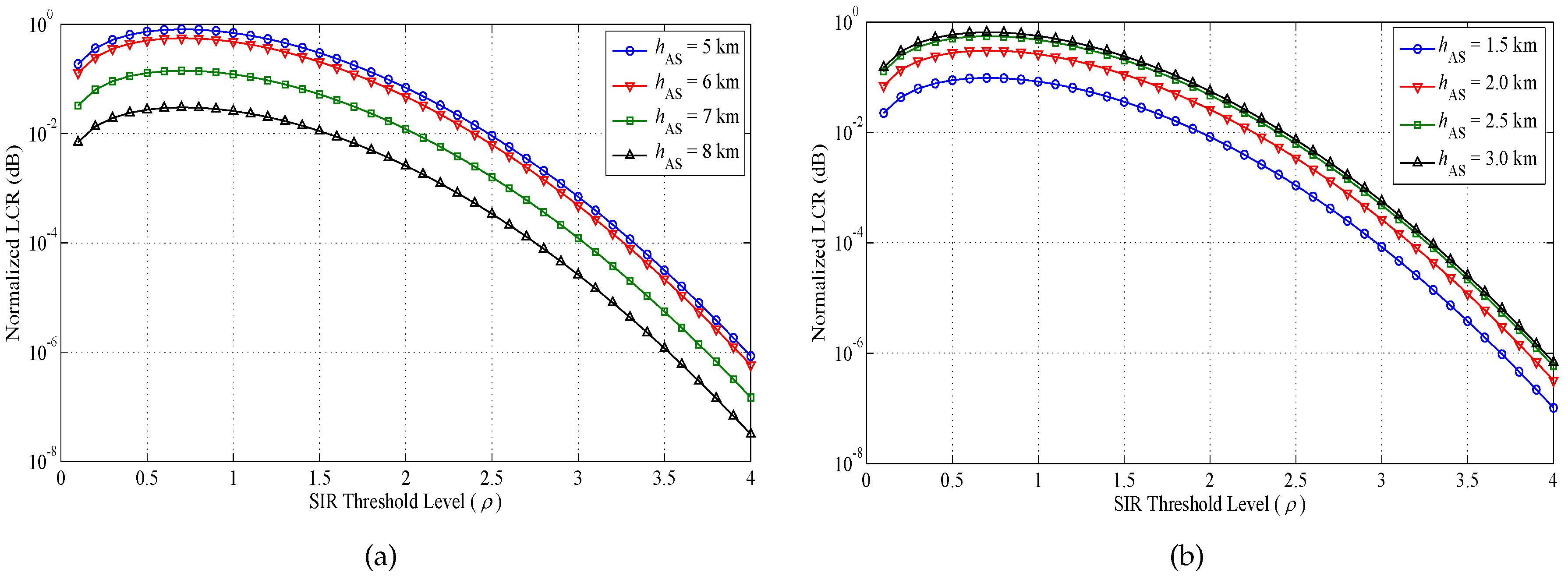
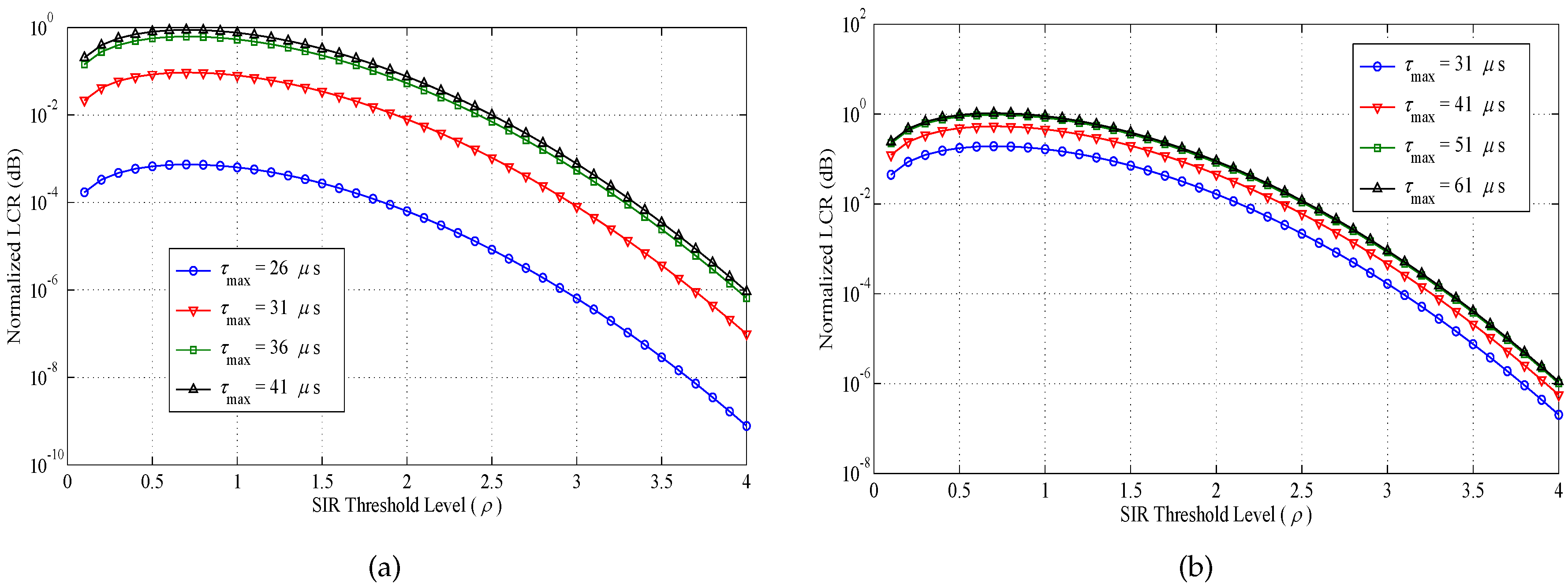
A detailed analysis on the second order statistics of the A2G channel is presented. The impact of major parameters, such as the height of AS, the longest propagation path’s delay and maximum Doppler frequency on these fading statistics, is analysed. The plots of the normalised LCR against the threshold level observed from AS and GS for different heights of AS are shown in Figure 11a,b, respectively. The LCR observed from AS increases gradually with the increase in the threshold level up to a certain level, and then, it decreases with the further increase in the threshold level. However, LCR decreases by increasing the height of AS, because LCR is sensitive to the density of scatterers, and AS is assumed as a scattering-free region. The LCR observed from GS is showing the same behaviour with respect to the threshold level as observed from AS, but it shows a converse trend with respect to the height of AS. The plots of the normalised LCR against the threshold level observed from AS and GS for different values of ${\tau }_{\max }$ are shown in Figure 12a,b, respectively. The LCR observed from AS increases gradually with the increase in the threshold level up to a certain level, and then, it decreases with the further increase in the threshold level. However, LCR decreases by reducing ${\tau }_{\max }$, and the rate of decrease is changed rapidly by reducing the ${\tau }_{\max }$, because AS moves away from GS. The LCR observed from GS is showing the same behaviour with respect to the threshold level, as well as with respect to ${\tau }_{\max }$. However, when the projection of AS on the x-y plane lies inside the TESR, LCR increases up to a level because of the density of scatterers and then almost remains constant for the further increase in ${\tau }_{\max }$. 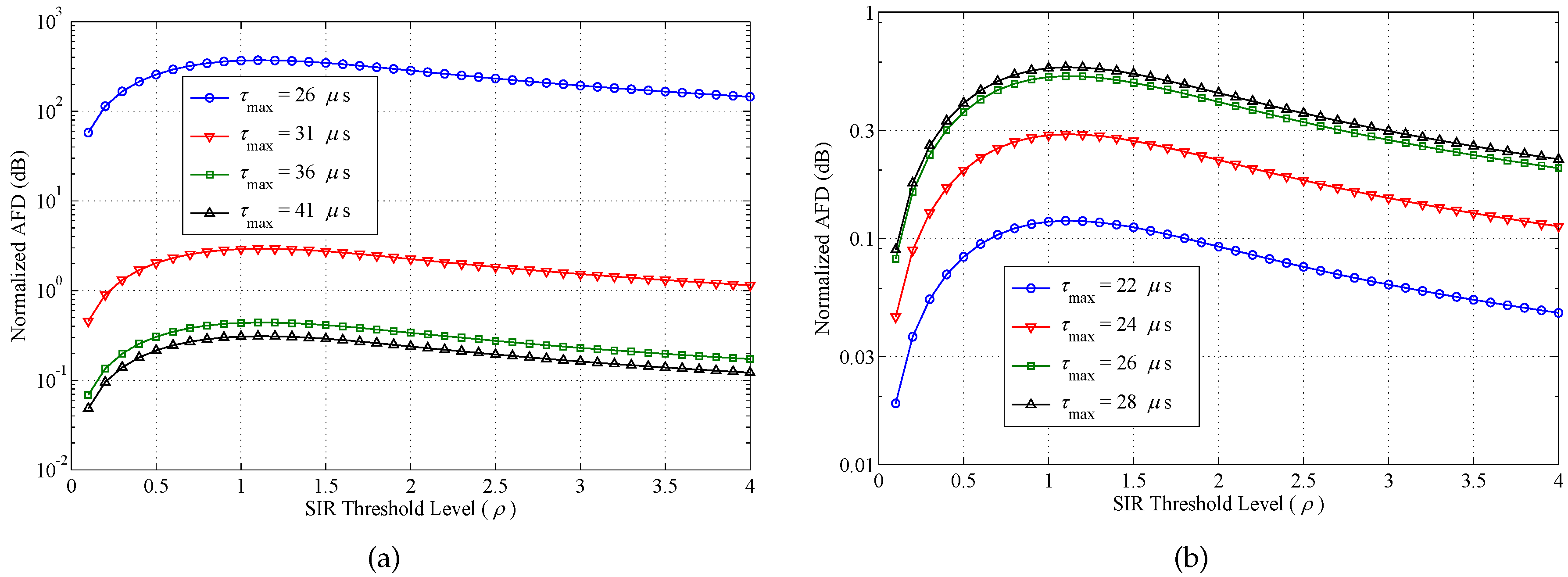The plots of the normalised AFD against the threshold level observed from AS and GS for different values of ${\tau }_{\max }$ are shown in Figure 13a,b, respectively. When observed from AS, AFD increases gradually with the increase in the threshold level up to a certain level, and then, it slightly decreases with the further increase in the threshold level. However, AFD increases by reducing ${\tau }_{\max }$, and the rate of increase is changed rapidly by reducing the ${\tau }_{\max }$ because AS moves away from GS. The AFD, when observed from GS, is showing the same behaviour with respect to the threshold level when observed from AS. However, when the projection of AS on the x-y plane lies inside the TESR, AFD increases with the increase in ${\tau }_{\max }$ up to a level because of the density of scatterers and then almost remains the same for the further increase in ${\tau }_{\max }$. 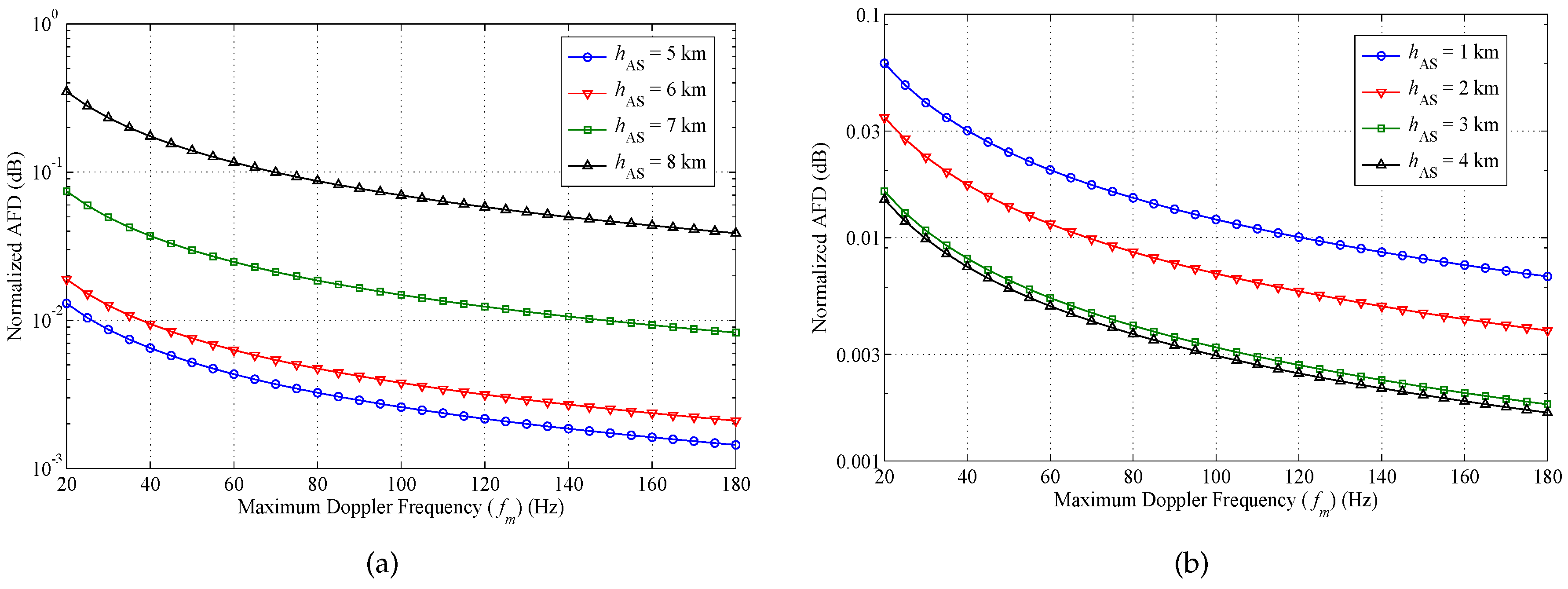The the plots of the normalised AFD against different values of the maximum Doppler frequency observed from AS and GS showing the effects of the height of AS are shown in Figure 14a,b, respectively. When observed from AS, AFD decreases smoothly with the increase in Doppler frequency. However, AFD increases by increasing the height of AS, and the rate of increase is higher with respect to the increase in the height of AS. Therefore, by increasing the height of AS, the projection of AS on the x-y plane moves out of the scattering region for a given delay; therefore, the number of multipaths is reduced, which results in the increase of AFD. The AFD, when observed from GS, is showing the same behaviour with respect to Doppler frequency, as observed from AS, but it shows the converse trend with respect to the height of AS.

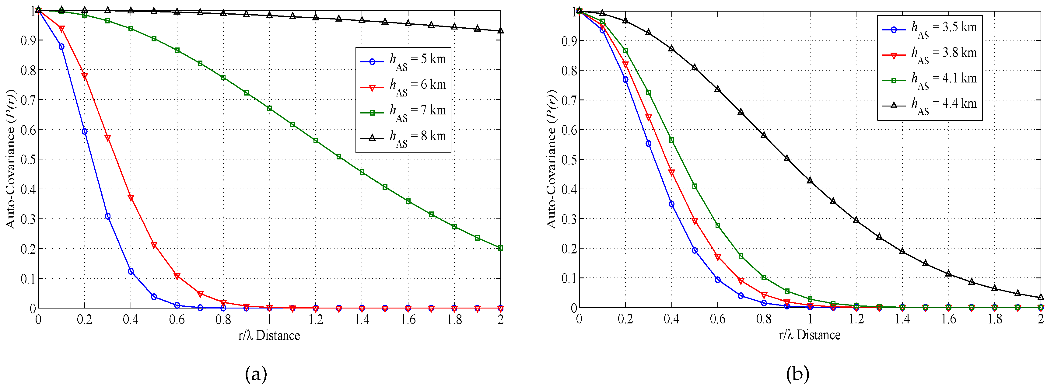
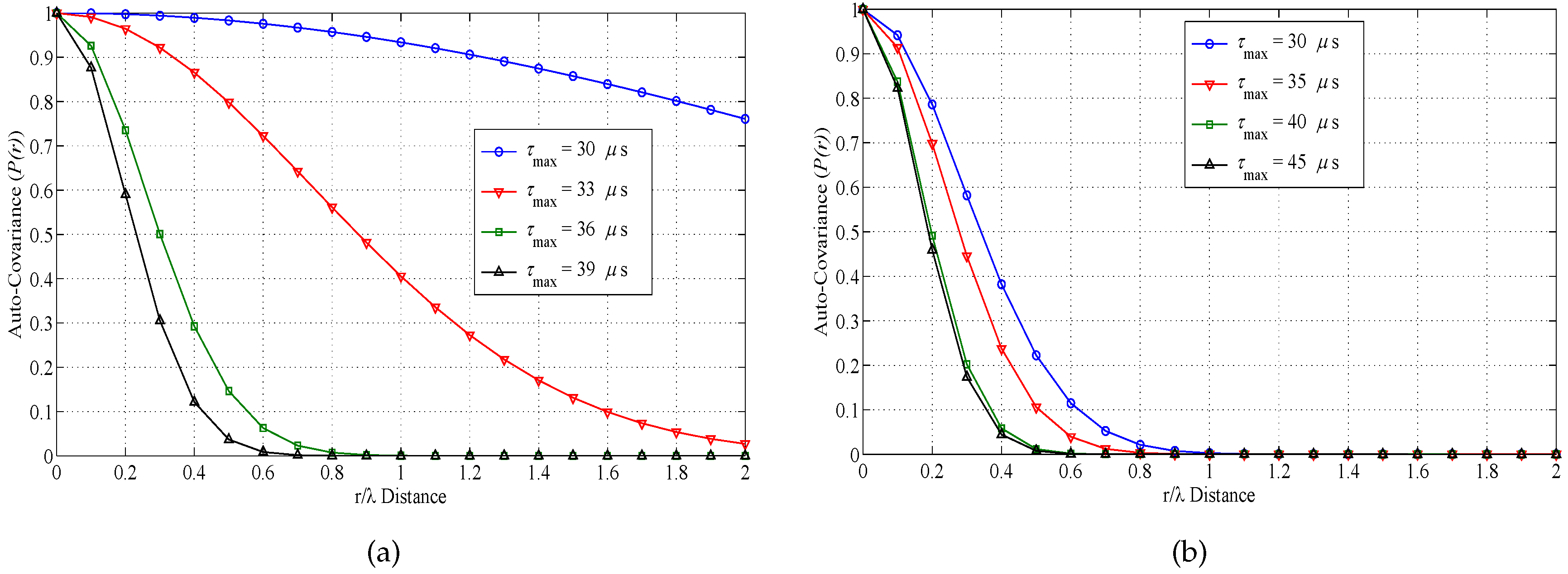
The results for auto-covariance against $r/\lambda$ observed from AS and GS for different heights of AS are plotted in Figure 15a,b, respectively. The auto-covariance decreases from one to zero with the increase in $r/\lambda$ distance, and it increases by increasing the height of AS because AS is moving away from GS for a given delay. The rate of increase changes rapidly with the increase in height of AS. For the height of AS at 8 km, it decrease from one to 0.9 only because for such an environment, the multipath components are received over a small angular range, which results in high correlation. However, for lower heights of AS, the projection of AS on the x-y plane lies inside the scattering region; multipath components arrive from a larger area, which results in lower correlation. When observed from GS, auto-covariance is showing the same behaviour as observed from AS. The results for auto-covariance against $r/\lambda$ observed from AS and GS for different values of ${\tau }_{\max }$ are plotted in Figure 16a,b, respectively. The auto-covariance decreases from one to zero with the increase in $r/\lambda$ distance and ${\tau }_{\max }$ because of the projection of AS on the x-y plane moves inside the TESR for a given height of AS. The rate of decrease changes rapidly with the increase in ${\tau }_{\max }$. When observed from GS, auto-covariance is showing the same behaviour as observed from AS.

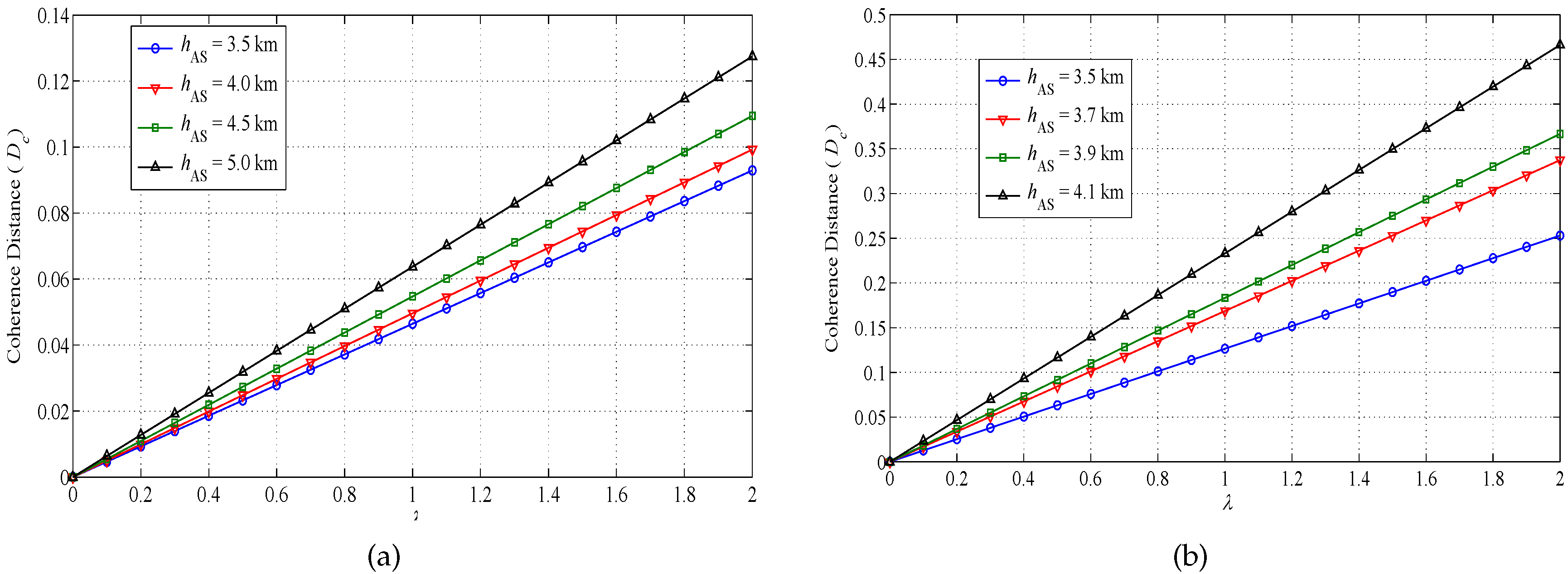
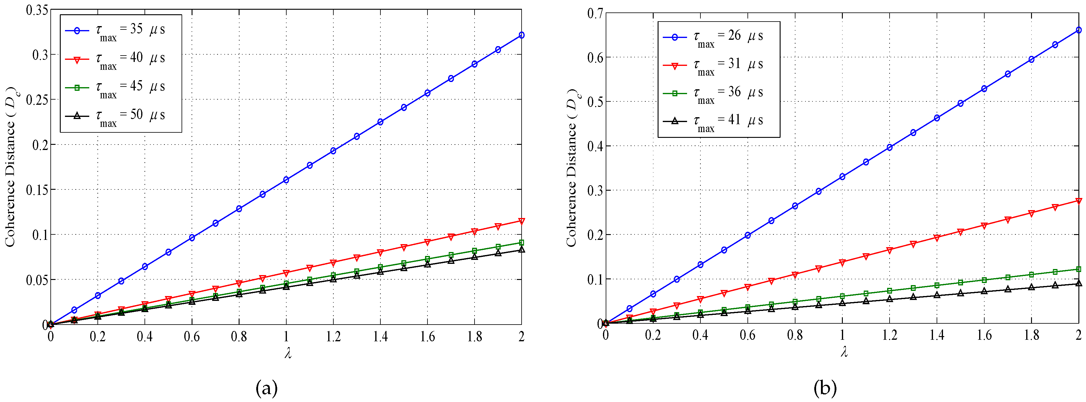
The results for coherence distance (${\mathit{D}}_{\mathit{c}}$), against λ observed from AS and GS for different heights of AS, are plotted in Figure 17a,b, respectively. The coherence distance gives information about the stability of the channel. The ${\mathit{D}}_{\mathit{c}}$ increases linearly with the increase in λ, and it is higher for high values of the height of AS because by increasing the height of AS, AS moves away from GS for a given delay. When observed from GS, ${\mathit{D}}_{\mathit{c}}$ is showing the same behaviour as observed from AS.

The results for ${\mathit{D}}_{\mathit{c}}$ against λ observed from AS and GS for different values of ${\tau }_{\max }$ are plotted in Figure 18a,b, respectively. The ${\mathit{D}}_{\mathit{c}}$ increases linearly with the increase in λ, but it decreases by increasing ${\tau }_{\max }$, because the shadow of AS on the x-y plane moves inside the TESR for a given height of AS. The rate of decrease changes rapidly with the increase ${\tau }_{\max }$. When observed from GS, ${\mathit{D}}_{\mathit{c}}$ is showing the same behaviour as observed from AS.

The proposed model is applicable for all of the altitudes of AS as long as $h_{\mathrm{AS}}$ > $h_{\mathrm{GS}}$ and $h_{\mathrm{AS}}$ > ${\sigma }_c$. The proposed analysis can be helpful in designing error control codes and diversity schemes required in future digital communication systems. LCR and AFD can also be used for the guidance of the selection of the packet length to minimize the packet error rate. The proposed analysis can be extended to devise AS’s velocity estimation algorithms by exploiting the relationship of LCR in (42), where it is evident that the maximum Doppler frequency is directly related to LCR, the spatial spread and other physical channel parameters. The proposed analysis on the coherence distance can be useful in studying the stability of the communication channels. The proposed analysis on the quantification of the spatial spread can be helpful in calculating the precise antenna correlations for designing efficient multi-antenna beamforming systems for future aeronautical communication networks.

6. Conclusions

A novel 3D geometric model has been proposed for the A2G/G2A radio propagation environments for the characterization of the Doppler spectrum and the spatial spread and the second order fading statistics. Mathematical expressions for joint and marginal PDFs of the Doppler shift, power and AoA have been derived. Furthermore, an analysis of SFs and second order fading statistics for A2G/G2A communication environments has been presented. The considered SFs are angular spread, angular constriction and the direction of maximum fading. The second order fading statistics considered in the presented analysis are LCR, AFD, auto-covariance and coherence distance. The SFs are computed using the knowledge of the PDFs of AoA and observed at both AS and GS in correspondence with both the azimuth and elevation planes. The second order statistics are computed using their relationship in terms of SFs. The impact of the azimuthal and elevational direction of AS’s motion, the height of AS, the height of GS and the delay of the longest propagation path on the distribution characteristics of the Doppler shift, SFs and second order fading statistics has been thoroughly analysed. To show the validity of the proposed model, a comparison of the proposed analytical results with the performed simulation results for the Doppler spectrum has been presented.

The proposed work can be used as a base to conduct a study for establishing a realistic choice of scattering objects’ distribution for spatial modelling of the vicinity of the ground station. The proposed work can also be used to study the impact of realistic antenna beam patterns on the channel characteristics.