1. Introduction
Fossil fuel is presently the major source for electricity production, and is believed to be a major contributor to greenhouse gas emissions. Burning of fossil fuel therefore has significant adverse environmental impacts. The general public and governments around the world are well aware of this. Enormous effort has therefore been put on the development and application of green energy sources. Wind is a promising alternative, which has the potential to be a major power source in future power systems. Huge investments are being made in this sector, which has led to considerable advancement in wind power technology. It is expected that wind power installations will grow substantially to produce clean energy in electric power systems. Another concern arises from the fact that the dwindling reserve of conventional fuel and increasing energy demand will eventually lead to rising prices of fossil fuel and other conventional energy generation. The installed capacity of wind farms in Canada is currently 6077 MW [
1]. Wind penetration, which is defined as the ratio of the installed wind capacity to the total installed capacity of a power system is currently about 2.3% in Canada. More than 6000 MW of additional wind capacity is expected to come into operation before 2015 [
1], increasing the penetration level to about 5%. It is a trend not only in Canada but all around the world. These statistics indicate that high levels of wind power penetration can be anticipated in the near future.
A wind turbine generator (WTG) converts wind energy into electric energy. Its operating characteristic is remarkably different than that of conventional electric energy sources. The output power of a WTG can vary over a wide range between zero and the rated capacity value, in a random but continuous fashion. The variation in power generation, and the uncertainty associated with the power output levels causes significant challenges in planning and operating a power system to meet the projected demand with an acceptable level of reliability. Different techniques have been used to model wind generation and integrate them to evaluate the reliability of wind-integrated power systems (WIPS).
There are basically two approaches for the quantitative reliability evaluation of a power system: Analytical techniques and Simulation techniques [
2]. Analytical technique [
2] is an approach to evaluate risk indices using mathematical models of system components with direct numerical solutions. References [
3,
4,
5] use analytical techniques for reliability evaluations. Simulation technique on the other hand, uses computer generated random numbers to represent system states. Risk indices are then calculated using the simulated system states over a long horizon of simulation time. Simulation techniques were used in [
6,
7,
8] for the reliability evaluation of WIPS.
Wind Power fluctuation is a major concern in maintaining system reliability as mentioned earlier. In WIPS connected to multiple wind farms, the correlations of wind speeds between different wind farms affect the variability of the overall wind power generation. A low wind speed correlation between the wind farms tends to result in reduced variability in combined power output characteristics, and vice versa. Correlation has a big impact on the fluctuations and should therefore be an important consideration in reliability modeling and evaluations. Some papers have incorporated the effect of correlations between multiple wind farms in reliability studies [
4,
5,
6,
7,
8,
9]. An auto-regressive time series based mathematical model for wind speeds of correlated wind farms was introduced in [
9]. Reference [
6] used auto regressive and moving average (ARMA) model to generate wind speeds of correlated wind farms by using correlated random number seeds and studied the impact of correlations on the adequacy indices of a WIPS using sequential Monte Carlo Simulation (MCS). The results showed that correlation has considerable impact in adequacy indices of a WIPS. Reference [
7] presented a genetic algorithm to obtain optimum random number seeds to generate wind speeds of correlated wind farms and used MCS to study the effect of wind penetration and correlation on system risk. Customized simulation programs and expertise in the field would generally be required to implement simulation techniques in practice, and therefore, would not be readily applied. The analytical method, on the other hand, is a relatively simple method, and should therefore be more attractive to system operators and planners. Reference [
4] introduced an analytical model of a WECS using conditional probabilities to obtain joint model of correlated WECSs. References [
7] and [
8] used this conditional method to build an analytical wind model. It becomes important to develop simple models to be readily acceptable in real world reliability evaluation applications. There have been studies done to reduce the number of states in multi-state models to simplify the evaluation. Reference [
10] suggested a simple seven-state analytical wind model. The correlation between multiple wind farms was, however, not considered in the study. The methods used in [
6,
7,
8,
9] to generate correlated random number seeds are quite complex. This paper uses a simple algorithm using Cholesky decomposition [
11] for the generation of correlated random numbers for recognizing correlation between two wind farms. This paper then focuses on simplifying the wind models incorporating the wind correlations and wind penetration levels.
2. Wind Data Modeling
It is very important to have a wind speed model that adequately represents the wind characteristics of a wind farm for wind energy studies. It has been shown in [
12] that the long term wind characteristics of a particular site can be represented by an ARMA model that can be written in the form of Equation (1):
where
Фi (
i = 1, 2, 3…s) and θ
j (
j = 1, 2, 3…m) are autoregressive and moving average coefficients of the wind model respectively. These coefficients can be calculated using the historical data of a site [
12].
αt is a Normally and Independently Distributed(NID) white noise process with zero mean and σ
2 variance generally expressed in the form
αt ∈NID (0, σ
2). Equation (1) represents a time series for
y, which can be generated using value of
αt randomly generated each time interval and previous values of
y and
α. An hourly time interval is used in this study. The time series of y obtained using Equation (1) can then be used to calculate the simulated hourly wind speeds using Equation(2).
where
SWt = Simulated wind speed for hour
t. µ
t = Hourly mean wind speed for hour
t. σ
t = Hourly standard deviation of wind speed for hour
t.
It should be noted that there are each of 8760 hourly mean and standard deviation values for a wind site obtained from its historical data. An ARMA model for Swift Current site, which is located in Saskatchewan, Canada is presented in [
12] and expressed in Equation (3).
αt can be generated using a suitable normally distributed random number generator. For the initial four calculations,
i.e.,
y1 to
y4, the preceding values of y and
α that at the right hand side of Equation (3) were assumed to be zero if they were not yet obtained.
Two sites each having the wind characteristics of Swift Current as represented by Equation (3) are considered in this work. Independently simulating the two sets of wind speed data using Equation (3) resulted in correlations being close to zero. The two sets of wind speed data are therefore simulated with random numbers in such a way to obtain a desired correlation between the two sites. The impact of wind correlation on the system reliability is then investigated. Correlation between two sets of simulated wind speed data can be established by using correlated random numbers during the hourly simulation [
6]. The correlation between the two sets of simulated wind speed data thus obtained is close to the correlation between the random numbers used. Various methods are available that can be used for the generation of correlated random numbers. The Cholesky Decomposition [
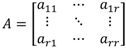
11] method is used in this paper. Cholesky Decomposition is the process of decomposing any symmetric and positive definite matrix into the product of two triangular matrices as represented by Equation (4).
where, A = A symmetric positive definite matrix, G = An upper triangular matrix with positive diagonal entries. G
T = Transpose of matrix
G.
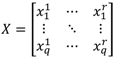
A set of
r uncorrelated random number series may be represented by matrix
X shown in Equation (5).
where, each column of matrix
X is an uncorrelated random number series with
q members. The desired correlation between any two sets of series may then be represented by Equation (6).
where,
aij is the desired correlation between
ith and
jth column of matrix
X. Upper triangular matrix
G can then be calculated using Cholesky Decomposition. Matrix
Xc which contains p correlated random number series as defined in matrix A can be deduced using Equation (7).
This method can be simplified when only two random number series are present as shown in Equation (8).
where,
X1 and
X2 are series of uncorrelated random numbers.
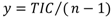
ζ is the desired correlation coefficient. Series
Xc calculated using Equation (8) has a correlation of
ζ with series
X1. A particular case was considered taking
ζ = 0.5. The scatter plots of 1000 pairs of uncorrelated and correlated random numbers thus obtained are compared in
Figure 1.
Figure 1.
Generation of correlated random numbers using Cholesky decomposition, (A) Uncorrelated random numbers; (B) Correlated random numbers with ζ= 0.5.
Figure 1.
Generation of correlated random numbers using Cholesky decomposition, (A) Uncorrelated random numbers; (B) Correlated random numbers with ζ= 0.5.
Two separate wind speed series can be synthesized using correlated random numbers
X1 and
Xc in Equations (2) and (3). The hourly mean and hourly standard deviation values of Swift Current site were obtained from Environment Canada. Two pairs of wind speed data series were simulated using
ζ = 0 and
ζ = 0.5. The scatter plots for 1000 data pairs for two cases are shown in
Figure 2.
Figure 2.
Simulated wind speeds using uncorrelated and correlated random numbers. (A) Using uncorrelated random numbers; (B) Correlated random numbers with ζ= 0.5.
Figure 2.
Simulated wind speeds using uncorrelated and correlated random numbers. (A) Using uncorrelated random numbers; (B) Correlated random numbers with ζ= 0.5.
It can be seen from
Figure 1 and
Figure 2 that the pairs of wind speed series simulated using Equations (2) and (3) have a correlation close to the correlation of the random numbers used. The actual correlation between the two pairs of simulated wind speed series using random numbers with
ζ = 0 and
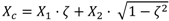
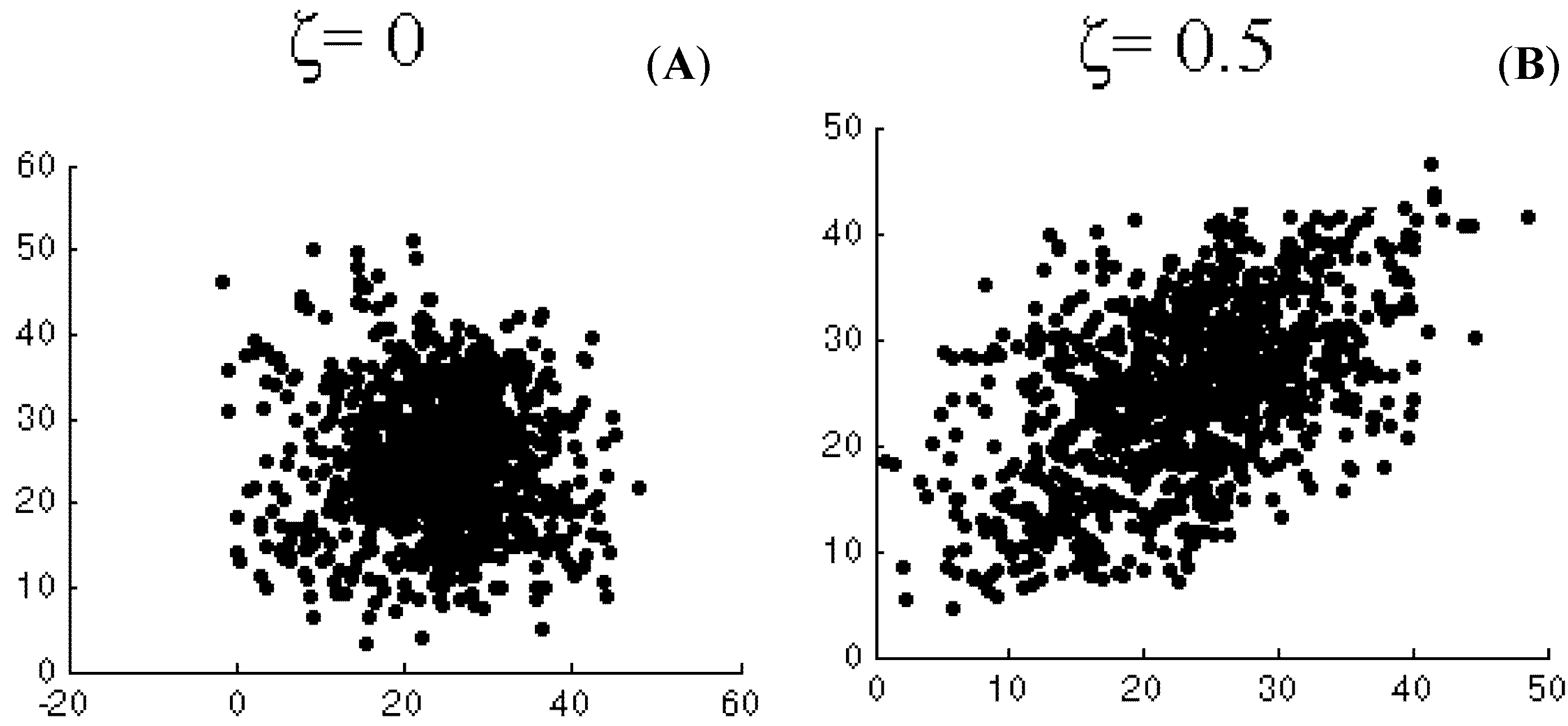
ζ = 0.5 were 0.11 and 0.56 respectively. The wind speed profile for the 21st and 22nd day are shown in
Figure 3 and
Figure 4 respectively for the two cases to illustrate how the wind speeds follow each other at the two correlation levels.
Figure 3.
2-day sample simulation of wind speeds for two sites with correlation of 0.11.
Figure 3.
2-day sample simulation of wind speeds for two sites with correlation of 0.11.
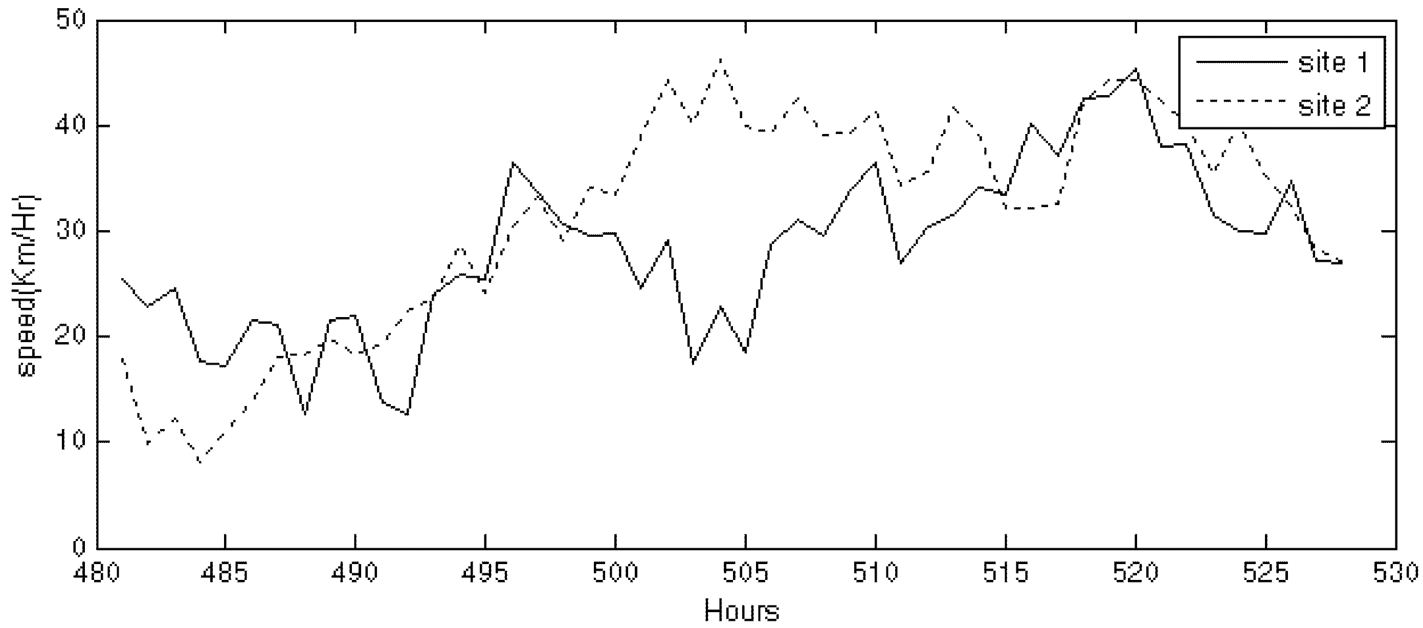
Figure 4.
2-day sample simulation of wind speeds for two sites with correlation of 0.56.
Figure 4.
2-day sample simulation of wind speeds for two sites with correlation of 0.56.
Wind speeds in
Figure 4 follow each other more closely than the ones in
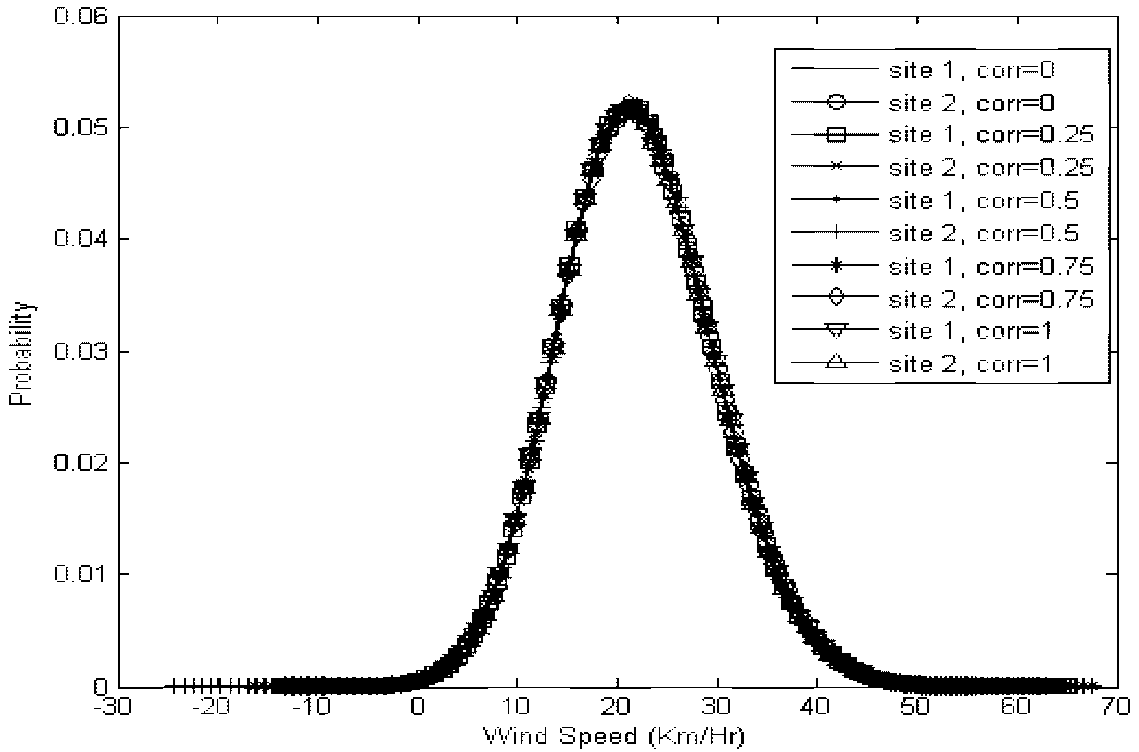
Figure 3 due to the induced correlations. The actual correlations obtained in simulated wind speeds of two sites were very close to the correlations of random numbers used. Pairs of correlated wind speed data were simulated with correlations 0, 0.25, 0.5, 0.75 and 1 using the same ARMA model of Swift Current for 8000 sample years. The probability distribution of wind speed for all of the generated series with varying correlation is given in
Figure 5.
Figure 5.
Probability distribution of wind speeds simulated at different correlations.
Figure 5.
Probability distribution of wind speeds simulated at different correlations.
It can be seen in
Figure 5 that the simulated wind speeds for two sites have almost identical probability distributions even if they have different correlations because of the use of same wind characteristic for both sites. Some of the simulated speeds obtained from above method are negative in magnitude, which cannot be defined. Different methods to deal with negative values produced during simulation are presented in [
10]. A straight forward method proposed by [
10] is to set all the negative values to zero after the completion of simulation process that has been used in this paper.
3. Wind Power Modeling
The output power of a WTG at any time depends on wind speed of the site at the time, forced outage rate (FOR) and the characteristics of the WTG influenced by the cut in, rated and cut out speed. Cut-in speed (
Vci) is the minimum wind speed that is required for a WTG to generate any power. Rated speed (
Vr) is the wind speed required for a WTG to generate maximum or rated power. Cut-out speed (
Vco) is the maximum wind speed that the WTG can safely handle,
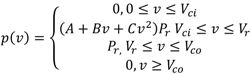
i.e., the WTG is shut down for safety reason at the cut-out speed. The relationship between wind speed (
v) and the corresponding output power of a WTG is presented in [
3] and can be expressed as Equation (9).
where
Pr is the rated capacity of the WTG, and constants A, B and C depend on
Vci,
Vr and
Vco [
3]. The
Vci,
Vr and
Vco of 14.4 km/h, 46.8 km/h, and 90 km/h respectively were used in this study. The simulated hourly wind speeds were converted to hourly power output values using (9). The effect of the FOR of the WTGs in a wind farm can be considered in the evaluation of the power output model of the wind farm. It has however been shown in [
13] that the FOR of a WTG can be neglected during reliability evaluation of WECS without losing reasonable accuracy. The effect of FOR has therefore been neglected in this study to simplify the wind model. Another assumption that has been made in this study is that all the WTGs in a wind farm experience same amount of wind speed in any particular hour. Five pairs of hourly power output series were developed using the above mentioned procedure for correlations of 0, 0.25, 0.5, 0.75 and 1. Both the wind farms were assumed to have equal installed capacities for all the cases in this study. The total hourly power generated by two wind farms denoted by
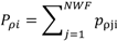
Pρi can be calculated using Equation (10).
where
pρji = power output of wind farm
j at hour
I;
i = 1 to 8760 ×
N;
N = number of simulated years.
NWF = number of wind farms considered.
ρ = correlation between wind farms which can be in the form a correlation matrix if more than two wind farms are considered.
The wind power series for multiple sites can be obtained using this process in which the time chronology and the cross-correlation between wind power outputs are maintained. Hourly power generation obtained by above method can then be grouped into suitable number of class intervals in ascending or descending order to obtain the wind capacity model. This model is a probability distribution of different capacity output states which is generally expressed as a capacity outage probability table (COPT) [
2]. Sturges’ Rule [
14] can be used to determine the appropriate number of class intervals, NoCI while grouping these data calculated using Equation (11).
where, (8760 ×
N) is the number of data points considered.
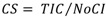
The number of class intervals for 8000 sample years calculated from Equation (11) is therefore 27. The class size CS is calculated using Equation (12):
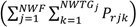
where, TIC =
![Applsci 03 00107 i016]()
is the sum of the installed capacities of all the wind farms connected to a power system;
Prjk = installed capacity of
WTG k in wind farm
j;
NWTGj = number of
WTG in wind farm
j.
The wind capacity model is represented by a COPT with NoCI capacity states. The capacity outage,
COi for a state
i is given by Equation (13). The probability of
COi outage state,
P (
COi) is given by Equation (14):
where
DPi is the number of wind power data points in the interval
i.
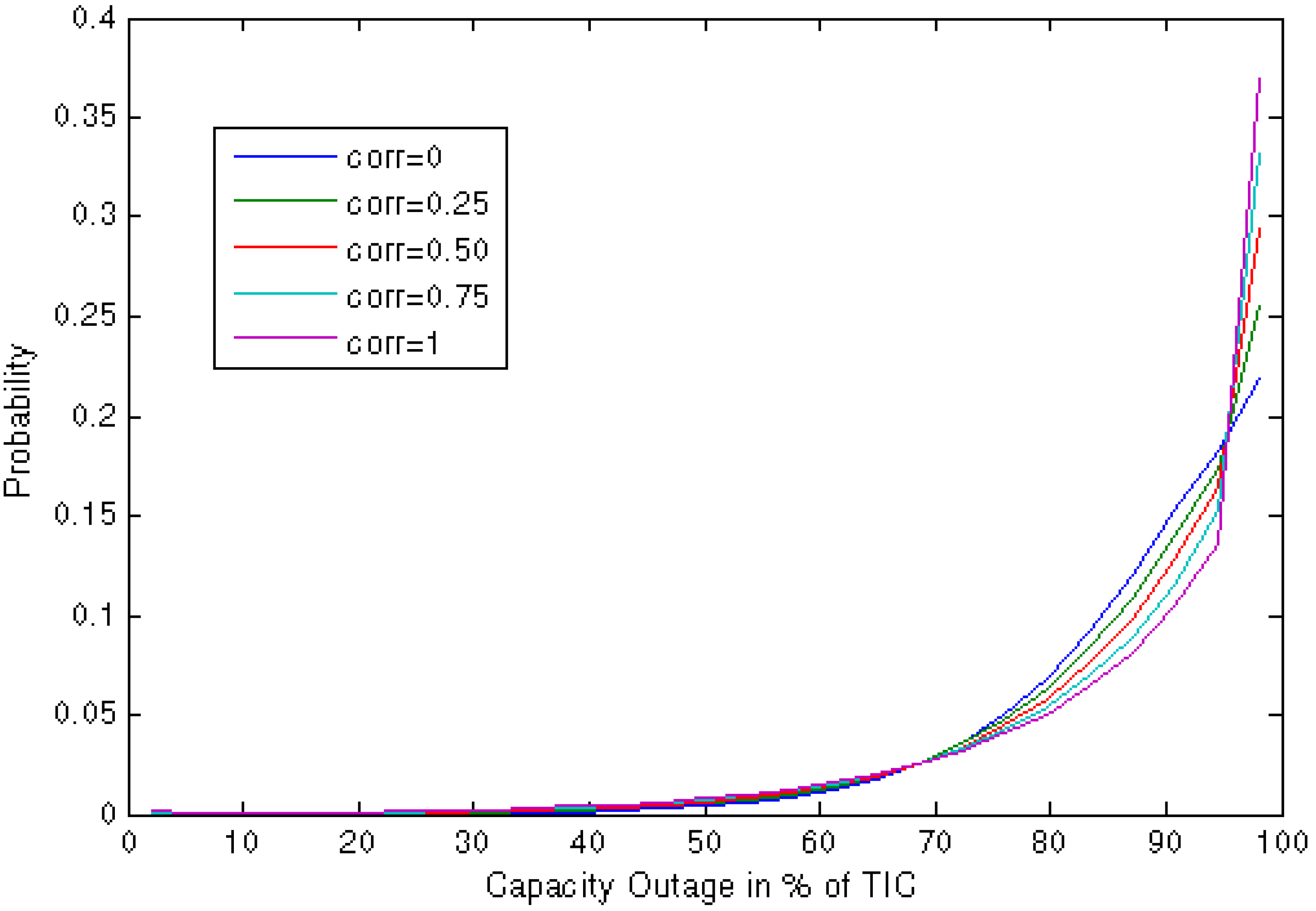
A 27-state wind capacity model for a WIPS containing two wind farms each rated at 425 MW was obtained using Equations (13) and (14). Both the sites were assumed to have wind profiles represented by the Swift Current, Saskatchewan wind data.
Figure 6 shows the wind capacity models considering five different correlations of 0, 0.25, 0.5, 0.75 and 1 between the two wind farms. The different correlations between the two sites were created using the method in Equation (8)
Figure 6.
27 state COPT for different wind speed correlations.
Figure 6.
27 state COPT for different wind speed correlations.
The 27-state capacity model can be simplified by reducing the number of capacity states using an apportioning method presented in [
15]. The step size of the reduced capacity model,
y is given by Equation (15).
where,
n is the number of states (NoS) of the reduced COPT.
The denominator in equation (15) is taken as (n−1) so as to include 0% and 100% of TIC in n-state COPT. The capacity outage levels of the reduced COPT are thus the multiples of y from zero to (n−1). The 27-state capacity model was reduced by successively decreasing n from 27 up to 5.
4. Impact of Wind Penetration and Correlation
The IEEE Reliability Test System (IEEE-RTS) [
16] was used in this study to investigate the effect of various factors on the reliability indices of a WIPS obtained using multi-state wind models. The IEEE-RTS has 32 generating units ranging from 12 MW to 400 MW capacities with a total installed capacity of 3405 MW. The system LOLE of IEEE-RTS is 9.44 h/year. The system peak load is 2850 MW. The details of load data are provided in [
16] from which the daily and hourly load models can be obtained. A Computer program called SIPSIREL [
17] was used to calculate LOLE values in this study. The LOLE of the IEEE-RTS decreases after adding wind generation to the system. The LOLE values obtained for the various correlation between the two wind farms, and to different wind penetration levels are summarized
Table 1.
Table 1.
LOLE values for RTS varying correlation and penetration.
Table 1.
LOLE values for RTS varying correlation and penetration.
| Correlation | Penetration |
|---|
| 5% | 10% | 15% | 20% |
|---|
| 0 | 8.1065 | 6.9114 | 5.9108 | 5.0427 |
| 0.25 | 8.1121 | 6.9442 | 5.9772 | 5.1453 |
| 0.5 | 8.1186 | 6.9803 | 6.049 | 5.2543 |
| 0.75 | 8.1231 | 7.0133 | 6.1161 | 5.3572 |
| 1.0 | 8.1263 | 7.044 | 6.1798 | 5.4549 |
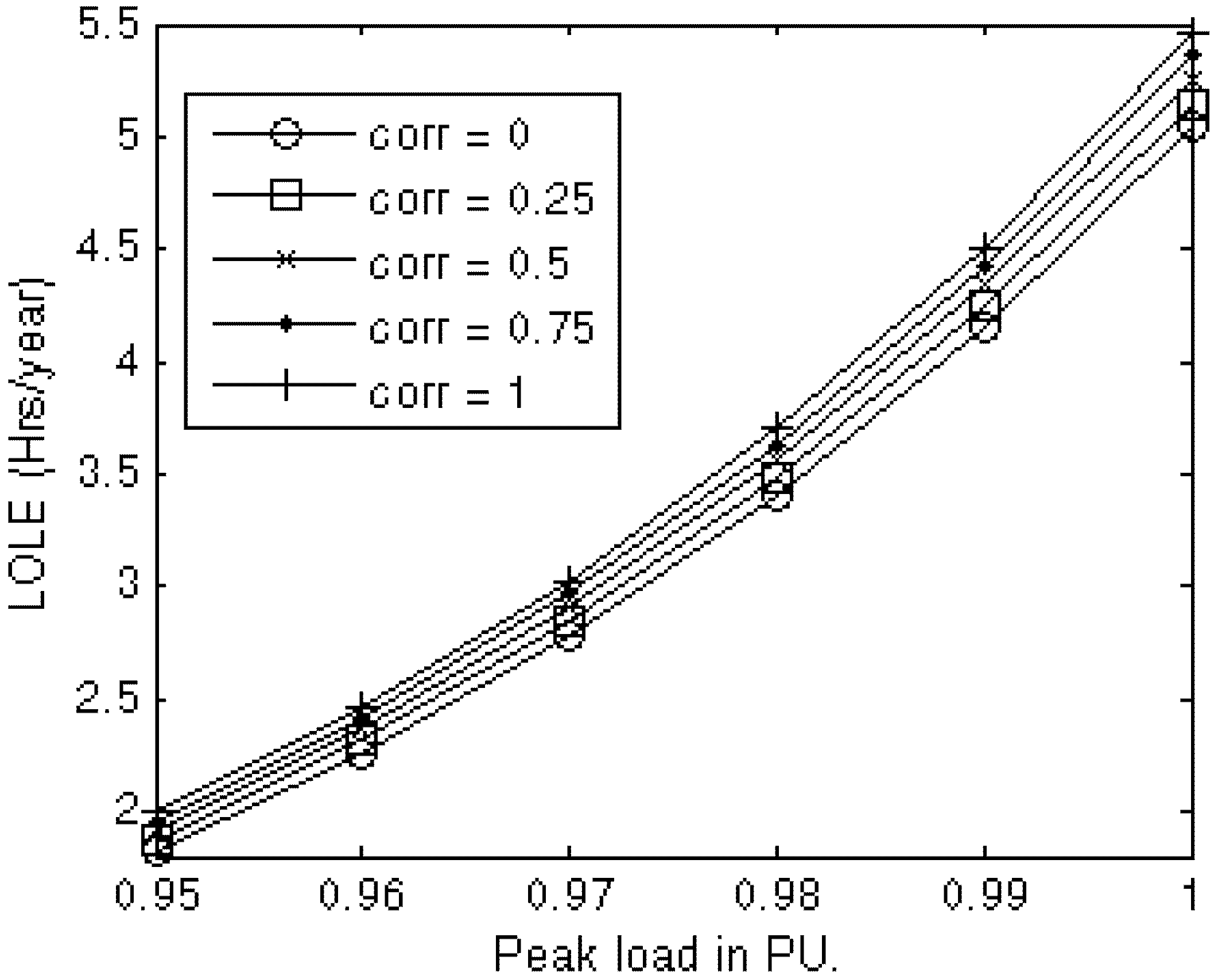
The impact of wind correlation on the WIPS reliability is shown in
Figure 7 by applying a 27-state wind capacity model to the IEEE-RTS with 20% wind penetration. The total wind capacity in this case is 850 MW from two wind farms of equal installed capacities connected to the system.
It can be seen in
Figure 7 that the system LOLE increases with the value of the correlation coefficient between the two wind farms, and vice-versa. Correlation between wind farms is therefore an important consideration in developing an appropriate wind model for reliability studies.
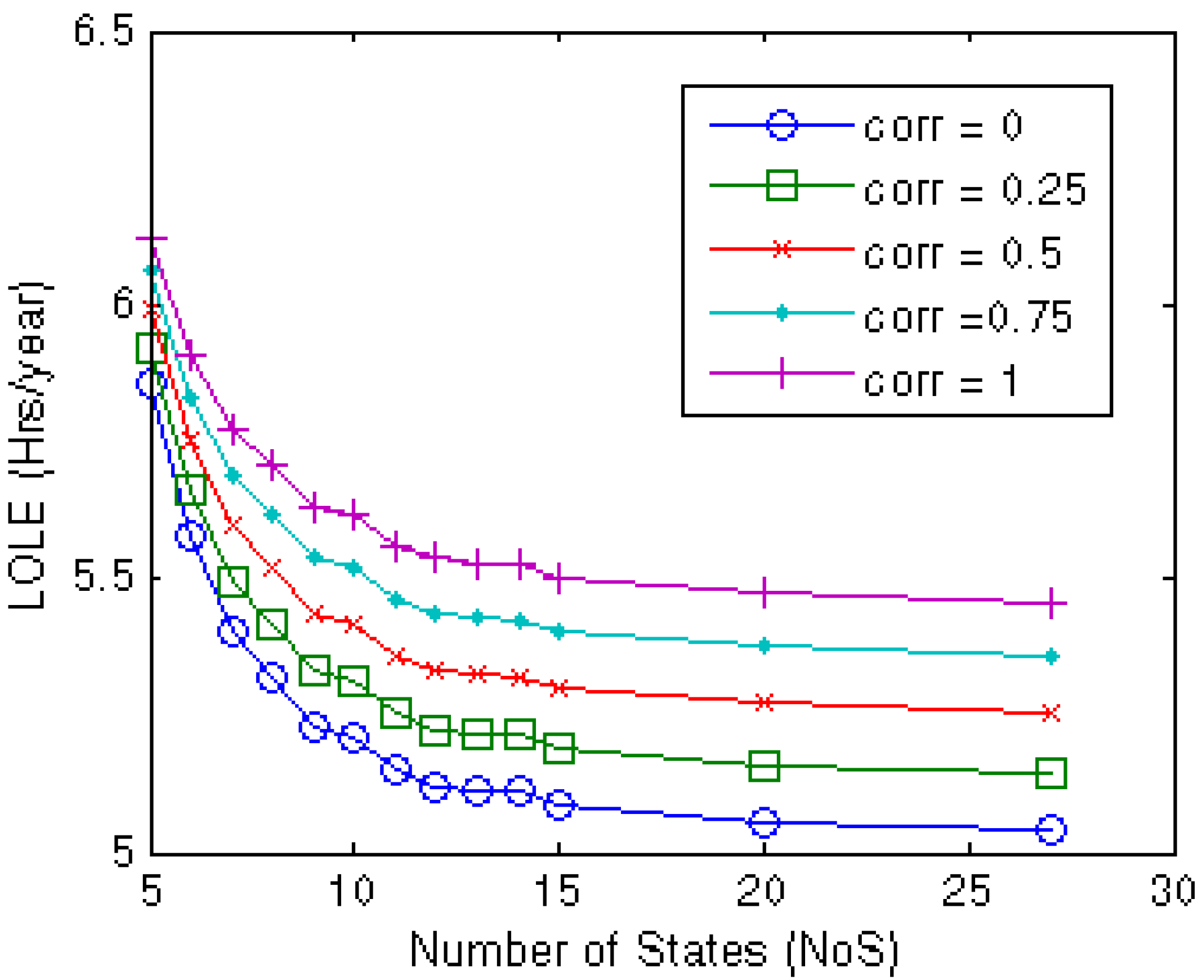
The multiple-state wind capacity model was simplified by gradually reducing the number of states from 27 to 5. The LOLE for the same system was evaluated for the different wind correlation values as described in the previous study. The WIPS LOLE for different number of states in the wind capacity model are shown in
Figure 8. It can be observed from
Figure 8 that he LOLE results obtained using a reduced number of states in the wind model can have remarkable error. The error rapidly increases as the NoS is reduced below 10 in this study. The results obtained from 27-state model are considered to be the most accurate in this study.
Figure 7.
Variation in LOLE with peak load for different correlations.
Figure 7.
Variation in LOLE with peak load for different correlations.
Figure 8.
Variation in LOLE results with the NoS in the wind model at different wind correlations.
Figure 8.
Variation in LOLE results with the NoS in the wind model at different wind correlations.
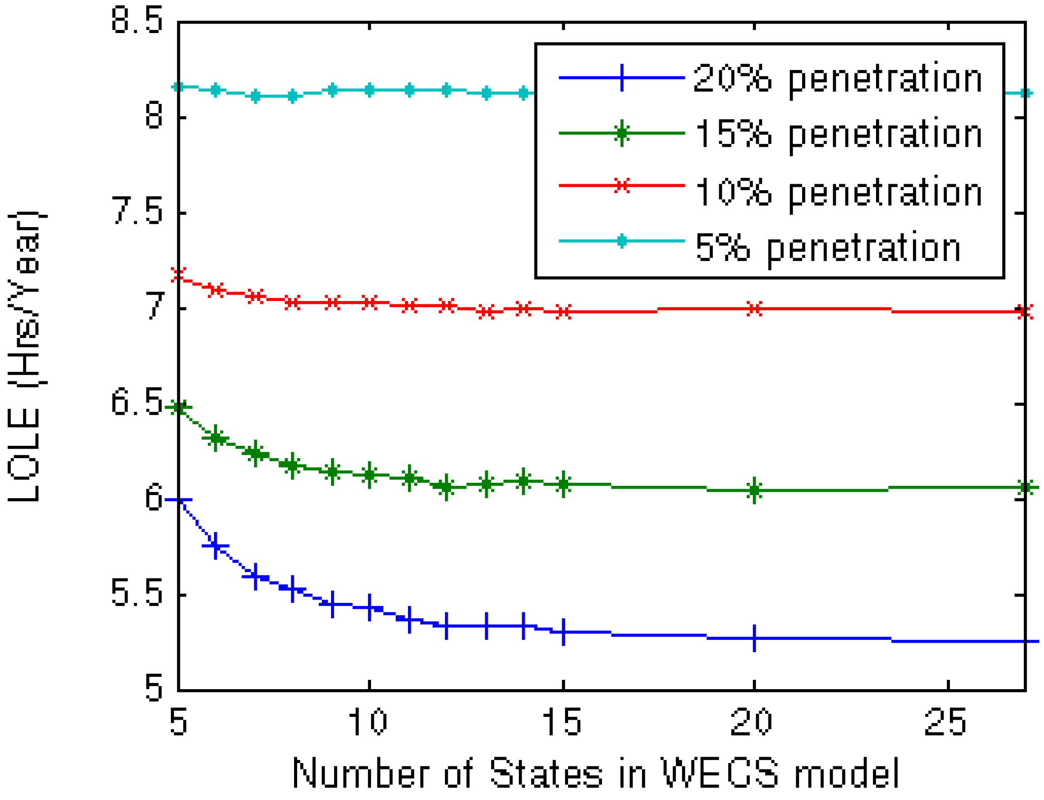
The impact of wind penetration on the LOLE accuracy obtained using different number of states in the wind model was also studied considering 5%, 10%, 15% and 20% wind penetration in the IEEE-RTS. The correlation between the wind farms was taken to be 0.5 in this case. The WIPS LOLE for the varying number of states in the wind capacity model at the different wind penetration levels are shown in
Figure 9.
It can be seen from
Figure 9 that the error in LOLE increases as the NoS is reduced. The increase in error is less significant at low wind penetration, and very significant at high penetration. It can be inferred from
Figure 9 that the determination of an appropriate NoS in the wind capacity model also depends upon the wind penetration level in a power system.
Figure 9.
Variation in LOLE results with the NoS in the wind model at different wind penetrations.
Figure 9.
Variation in LOLE results with the NoS in the wind model at different wind penetrations.
5. Appropriate Wind Capacity Model Considering Wind Correlation and Penetration
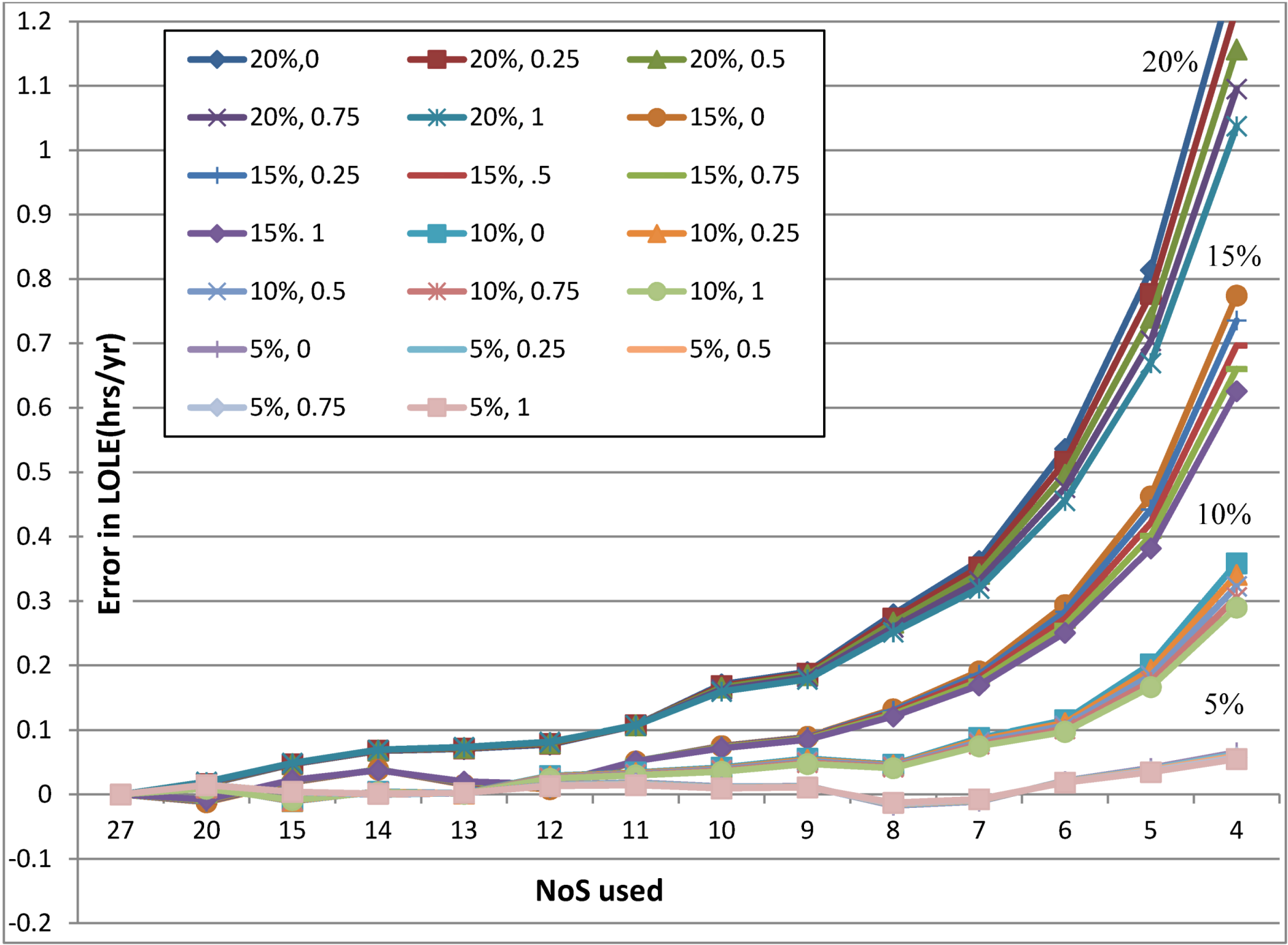
Table 1 presented the reliability evaluation results considering different wind penetrations in the IEEE-RTS at different correlations between the two wind farms connected to the system. The results were obtained using a 27-state wind capacity model. Similar studies were carried out using wind capacity models with reduced number of states. Reducing the number of states in the wind model simplifies the evaluation process at the cost of accuracy in the results. The errors in the WIPS LOLE obtained using reduced wind models at different wind penetrations and wind farm correlations were calculated using the
Table 1 results obtained from the 27-state model as the reference. The results are shown in
Figure 10.
It can be seen in
Figure 10 that the error in LOLE results generally increases as the number of states in the wind capacity model is reduced. The error is insignificant up to a certain NoS reduction, and then increases sharply as the NoS are further reduced. The error resulting from a reduced NoS is very sensitive to the wind penetration level. The errors increase rapidly as wind penetration increases and the number of states are reduced for model simplification. This is an important observation since the wind penetration in many WIPS around the world is expected to substantially increase within the next decade.
Figure 10 also shows the impact of wind correlation on the LOLE errors obtained by using a reduced wind capacity model. At low wind penetration, the wind farm correlation does not really affect the LOLE errors as the NoS is reduced to simplify the wind model. The effect of correlation on the errors produced by NoS reduction is however significant at high wind penetration. The error increases as the correlation coefficient between the wind farms is decreased, and vice versa. The effect of correlation on the LOLE errors can be significant if relatively low NoS are used in the wind model at reasonable wind penetrations in the foreseeable future.
Figure 10.
Error produced by using reduced number of states in the Wind Capacity model.
Figure 10.
Error produced by using reduced number of states in the Wind Capacity model.
Highly accurate results are usually not desired in a practical world if the methodologies to obtain the results are difficult to apply. An easy to use method that provides results with reasonable accuracy is more suitable for real life application. A wind capacity model with the minimum number of states that produces reasonable accuracy should therefore be used in WIPS reliability evaluation. An evaluation model that can provide system LOLE results within an error of 0.1 h/year would be considered appropriate model in practice. The minimum NoS to simplify a wind capacity model can therefore be deduced from
Figure 10.
Table 2 shows the appropriate wind capacity model at three different wind penetration levels.
Table 2.
NoS for wind capacity model.
Table 2.
NoS for wind capacity model.
| Penetration Level | Minimum NoS |
|---|
| up to 10% | 7 states |
| up to 15% | 9 states |
| up to 20% | 11 states |
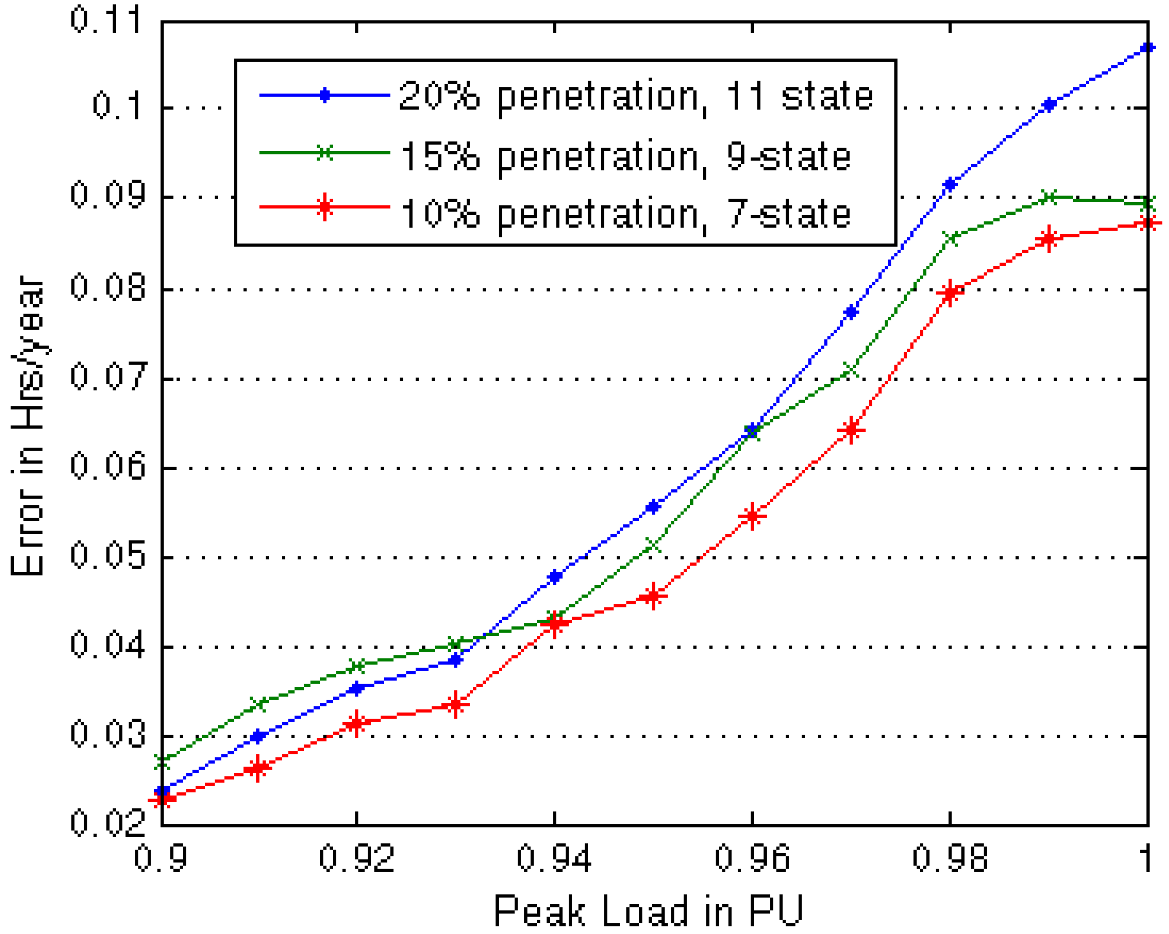
The wind capacity models recommended in
Table 2 were applied to the IEEE-RTS considering wind penetrations of 10%, 15% and 20% from two wind farms with zero wind correlation. It is shown in
Figure 10 that the error is highest when correlations between sites are zero. The LOLE of the IEEE-RTS without considering wind penetration is 9.44 h/year, which is relatively higher than the NERC recommended criterion of 0.1 day/year. This criterion is equivalent to about 1 h/year [
18]. The peak load of IEEE-RTS was reduced up to 90% to get LOLE values close to 1 h/year. The WIPS LOLE at the three wind penetration levels were calculated for a range of system loads between 90% and 100% of the IEEE-RTS peak. The errors in the system LOLE were calculated by comparing with the results obtained from the 27-state model, and are shown in
Figure 11.
Figure 11.
LOLE errors at different peak loads obtained using the recommended wind capacity models.
Figure 11.
LOLE errors at different peak loads obtained using the recommended wind capacity models.
It can be seen from
Figure 11 that the recommended wind capacity models provide results with acceptable accuracy at the different wind penetration levels. The error level is less than 0.03 h/year at a typical peak load level, which is 0.9 p.u. in the case of IEEE-RTS. This suggests that the wind models chosen are conservative for practical cases and may be used with confidence for reasonable accuracy.


 is the sum of the installed capacities of all the wind farms connected to a power system; Prjk = installed capacity of WTG k in wind farm j; NWTGj = number of WTG in wind farm j.

