Article

Biofuels and Land Use Change: Applying Recent Evidence to Model Estimates

Department of Agricultural Economics, Purdue University, 403 West State St. West Lafayette, IN 47907-2056, USA
*
Author to whom correspondence should be addressed.
Appl. Sci. 2013, 3(1), 14-38; https://doi.org/10.3390/app3010014
Submission received: 10 October 2012 / Revised: 4 December 2012 / Accepted: 6 January 2013 / Published: 11 January 2013
(This article belongs to the Special Issue Renewable Energy)

Abstract

:
Biofuels impact on global land use has been a controversial yet important topic. Up until recently, there has not been enough biofuels to have caused major land use change, so the evidence from actual global land use data has been scant. However, in the past decade, there have been 72 million hectares added to global crop cover. In this research we take advantage of this new data to calibrate the Global Trade Analysis Project (GTAP) model and parameters. We make two major changes. First, we calibrate the land transformation parameters (called constant elasticity of transformation, CET) to global regions so that the parameters better reflect the actual land cover change that has occurred. Second, we alter the land cover nesting structure. In the old GTAP model, cropland, pasture, and forest were all in the same nest suggesting, everything else being equal, that pasture or forest convert to cropland with equal ease and cost. However, we now take advantage of the fact that pasture converts to cropland at lower cost than forest. The paper provides the theoretical and empirical justification for these two model improvements. Then it re-evaluates the global land use impacts due to the USA ethanol program using the improved model tuned with actual observations. Finally, it shows that compared to the old model, the new model projects: (1) less expansion in global cropland due to ethanol expansion; (2) lower U.S. share in global cropland expansion; (3) and lower forest share in global cropland expansion.

Graphical Abstract

1. Introduction

Land use change induced by human activities is a major source of greenhouse gases (GHGs). Houghton [1] estimated that about 1/3 of carbon emissions released to the atmosphere since 1850 has resulted from land use change. Ramankutty and Foley [2] estimated that the average annual rate of deforestation was about 4.25 MH during the time period of 1850–1990. The annual rate of deforestation has increased to 8.3 MH in 1990s and then decreased to 5.2 MH during the past decade [3]. Expansion in cropland is the major source of land conversion and deforestation. Traditionally, the expansion in cropland has occurred to satisfy the need for higher demands for food and fiber products.
During the past decades several countries around the world have launched biofuel programs to produce renewable fuels from agricultural resources. Several papers have assessed the economic and environmental impacts of these programs. The early papers published in this area suggested that the USA corn ethanol program could cause major land use implications [4,5,6]. However, the more recent studies find that the early estimates have overstated the land use implications of this program [7,8,9,10,11,12,13].
While research studies in this area have distinguished and examined the important factors which determine the land use impacts of biofuels and their geographical distributions no attempt has been made to validate the land use estimates due to biofuels in the face of actual observations [14]. The reason is simple. Prior to the last couple of years, there was insufficient data on global land use change during the biofuels boom era. However, now we have that data, and it can be used to better calibrate prior estimates of land use change, which is the objective of this paper. The global biofuel programs, particularly the USA and EU mandates, took off in the early 2000s. However, prior to the past 5–6 years the level of biofuel production was very low and there was no way to get any idea of land use changes that might come about due to the much higher mandated levels of biofuels. In 2011, USA corn ethanol production was over 14 billion gallons, near the Renewable Fuel Standard (RFS) level of 15 billion gallons stipulated for 2015. In this year Brazil also produced about 6 billion gallons of sugarcane ethanol, and the EU members jointly produced more than 4 billion gallons of ethanol equivalent of biofuels (including ethanol and biodiesel). Thus, with these large magnitudes of biofuel production we should be able to see some impacts of land use change even if we still cannot isolate the biofuels induced part of that change with precision.
The existing estimates for the indirect land use change (iLUC) emissions due to biofuels are usually obtained from economic partial or general equilibrium models. To estimate iLUC emissions economic models, one way or another, estimate induced land use changes due to biofuel production. A land supply system which relates supply of different land types to their return or their land conversion costs is a key and common component of economic models used in this area. The existing Computable General Equilibrium (CGE) models usually use Constant Elasticity of Transformation (CET) functional forms to define their land supply system. Land transformation elasticities are needed to define a land supply system. These elasticities are difficult to directly estimate using econometric methods due to lack of sufficient quality data. In some circumstances the land transformation elasticities can be retrieved from the exiting land supply elasticity estimates [15] or can be estimated using simulated pseudo data [16]. A calibration or tuning practice is an alternative method which can be applied to tune land transformation elasticities for large and global CGE models [13]. In this paper we use observed information to tune the land transformation elasticities for the GTAP-BIO model.
This global CGE model, developed at the Center for Global Trade Analyses, has played a leading role in estimating biofuel induced land use changes. Several studies have used this model to evaluate iLUC emissions due to biofuels [7,10,11,12,17,18]. This model uses two different land transformation elasticities to govern the supply of land in each region. The first transformation elasticity (named ETL1) governs land allocation among managed forest, cropland, and pasture land. The second transformation elasticity (named ETL2) distributes available croplands among alternative crops. In the absence of regional empirical estimates for these elasticities, the model uses the same value for each of these parameters for all regions presented in the model.
Using similar land transformation elasticities for all regions presented in the model cannot be justified based on actual observations. As explained later on in this paper, historical observations confirm that regional land use changes followed different patterns during the past two decades. For example, historical data confirms the area of USA cropland remained constant during the past two decades, but its distribution among crops has changed significantly during the same time period. This indicates that no movement along land cover frontier has accrued in the USA during the past two decades, but movement along the cropland frontier occurred frequently in this economy. On the other hand, the area of cropland has expanded significantly in Sub Saharan Africa with relatively minor changes in its distribution among crops over the past two decades. Clearly these two patterns are not consistent with using the same land transformation elasticities for these two regions.
Furthermore, as shown in the top panel of Figure 1, the GTAP-BIO model puts three types of land cover items (forest, pasture, and cropland) in one nest and implicitly assumes that the economic costs of converting one hectare of forest to cropland is similar to the economic costs of converting one hectare of pasture land to cropland and vice versa. This set up is another key deficiency of the GTAP-BIO model. Including cropland, forest, and pasture land in the same nest could cause systematic bias in land conversion processes among land cover types due to biofuel production. In general this is not the case and often the opportunity costs of converting forest to cropland is higher than the economic costs of converting pastureland to cropland.
In this paper we remove these two deficiencies. We tune the regional land transformation elasticities based on actual historical observations on changes in land cover and distribution of cropland among alternative crops during the past two decades. To accomplish this task we use published data on cropland use around the world by the Food and Agricultural Organization (FAO) of the United Nation over the period 1990–2010. We alters the land cover component of the land supply tree, see the bottom panel of Figure 1, to have forest and pasture land in two different nests as described later in this paper. Then we re-evaluate the global land use impacts due to the USA ethanol program using the improved model tuned with actual observations. Finally, we show that compared to the old model the new model projects: (1) less expansion in global cropland; (2) lower share for the USA economy in global cropland expansion; (3) and lower forest share in global cropland expansion.
Figure 1. New and old land supply trees in GTAP-BIO model.
Applsci 03 00014 g001
In what follows, we first review the regional historical observations on cropland changes to distinguish regional land allocation patterns. Then we use the distinguished regional land allocation patterns to tune the GTAP-BIO land transformation elasticities based on actual observations. In the next step we alter the land cover frontier of the model. The next section defines our experiments to evaluate iLUC due to ethanol expansion using the new and old model. Then we present the simulation results. The last section provides conclusions.

2. Experimental Section

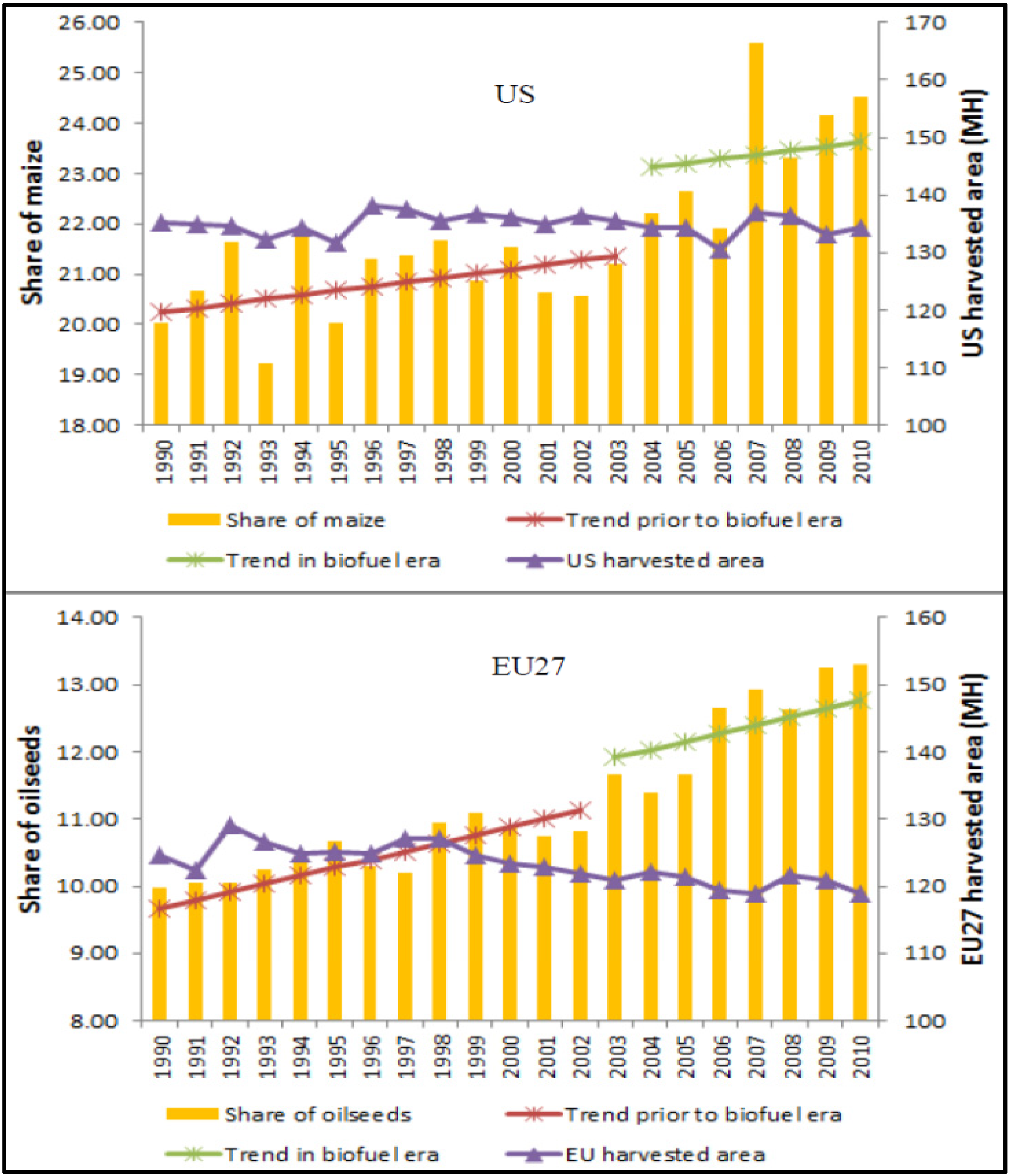
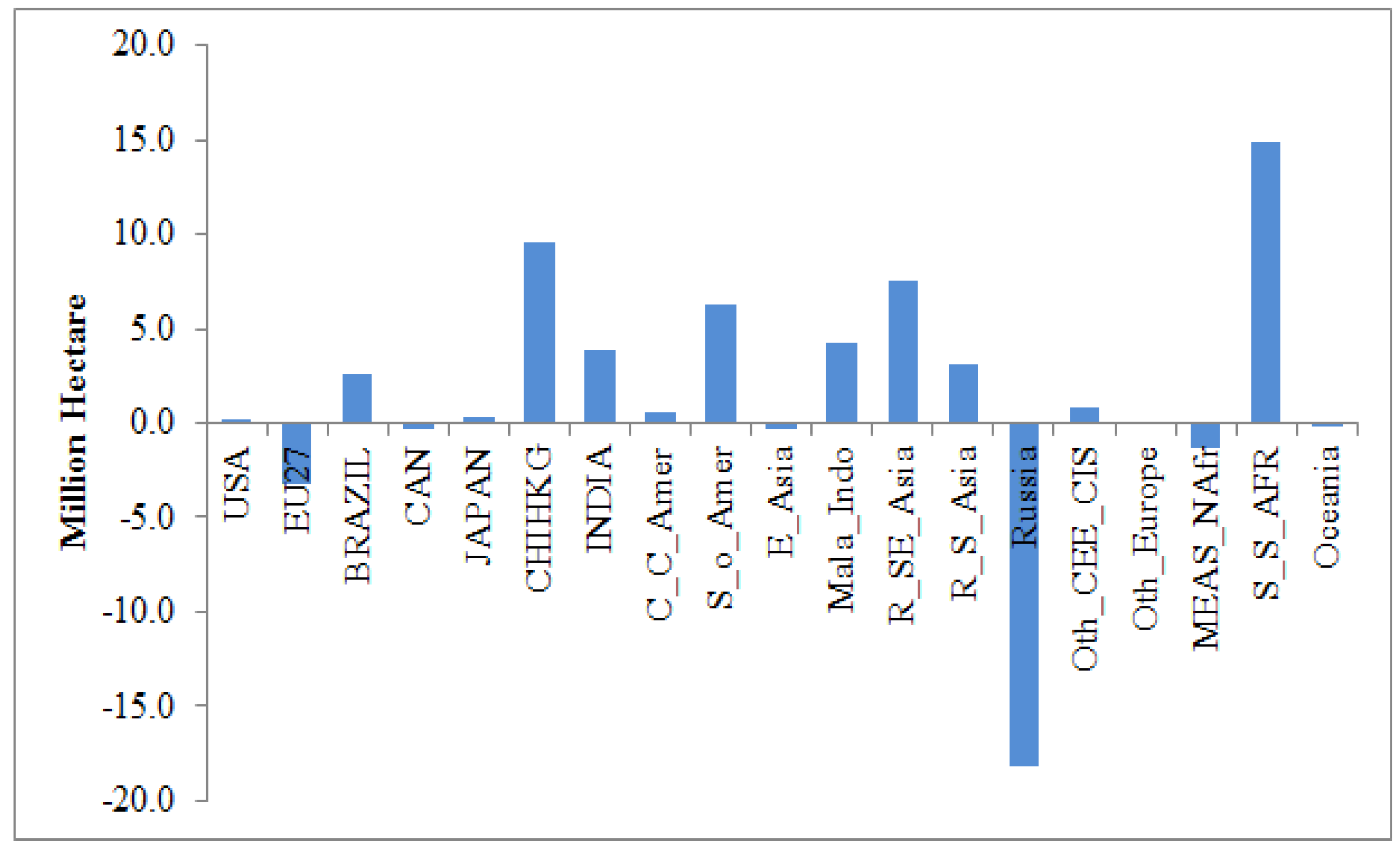
2.1. Evolution in Agricultural Land Use and Major Land Allocation Patterns in 1990–2010

This section uses two FAO data sets to examine global land use changes by region to reveal regional common land allocation patterns in response to changes in markets for agricultural commodities. The first set represents expansion and/or contraction in agricultural land (representing changes in cropland cover). In FAO data, pasture is included in cropland, so an expansion in cropland cover indicates deforestation and a reduction in cropland cover could represent reforestation and or conversion of agricultural land to other uses (e.g., expansion in urban areas). The second data set characterizes changes in harvested areas. An expansion in total harvested areas could be due to many factors. The harvested areas of a region may increase due to deforestation (expansion in crop cover), returning idled croplands to crop production, increases in double cropping, or reduction in crop failures. On the other hand total harvested areas may decrease in a region due to reduction in demand for crops, drought or other catastrophic events. In general, over a long time period total harvested area and land cover move together. However in the short run they may diverge. In this section we also use harvested areas to analyze changes in supply of land to alternative crops.
During the time period of 1990–2000 commodity markets were relatively stable, and in many countries agricultural activities were under governmental support programs. The agricultural markets experienced major changes in the next decade. Several countries (in particular, USA and EU members) reduced or modified their agricultural support programs during this decade. Biofuel production began to grow much faster around 2004 in many countries, especially USA, Brazil, and EU. Many counties, especially China and India, observed significant food demand expansion due to rapid economic growth. In addition, the crude oil price reached to its historical high with significant impacts on the production costs of agricultural products. In response to these changes, crop prices went up significantly and agricultural markets experienced major turbulences especially during the years 2008–2011. The higher commodity prices led to increases in cropland cover globally. The study of regional land use changes during these time periods, in particular after 2004, is the key to tuning the land transformation elasticities used in GTAP-BIO model.
The global area of agricultural land has increased by about 37.5 million hectares (MH) during the past two decades. During this time period the area of global forest has decreased by about 135 MH. These figures confirm land conversion along the land cover frontier at the global scale. On the other hand, the global harvested area followed a relatively flat trend in the 1990s, and then it sharply increased by about 71 MH during the next decades (from 1353 million hectares (MH) in 2000 to about 1424 MH in 2010 (Figure 2). This rapid growth in the global harvested area reflects major expansion in the demand for agricultural products during the time period 2000–2010.
Figure 2. Global harvested area 1990–2010.
Applsci 03 00014 g002
The allocation of cropland among alternative crops has changed significantly during the past two decades. Figure 3 summarizes changes in global harvested areas by crop for the past two decades (for the list of crop categories and their member see Table A1 in Appendix A). This figure indicates positive and large changes in the harvested areas of maize and oilseeds and negative and large changes in the harvested areas of crop categories of wheat, other coarse grains, and animal feed. From these observations we can conclude that global harvested area has increased significantly during 2000–2010. However, the rate of land conversion from forest to agricultural land has decreased in this time period compared to the time period of 1990–2000. Reduction in the area of global idled land, increase in double cropping, and reduction in crop failure could help explain the increase in harvested area while forest cover has decreased less.
Figure 3. Changes in global harvested area by crops (figures are in million hectares).
Applsci 03 00014 g003
Figure 4. Global harvested area by region trajectory.
Applsci 03 00014 g004
We now examine regional changes in agricultural land and harvested (the regional aggregation is taken from GTAP-GIO model and is presented in Table B1 in Appendix B). Figure 4 represents trajectories of harvested areas by region during the past two decades. In general, the 19 regions presented in this figure can be divided into three groups in terms of land conversion among land cover items and among alternative crops.
The first group includes regions or countries for which harvested areas have not changed extensively during the past two decades. However, in these countries allocation of cropland among alternative crops has typically changed over time. For example, during the past two decades the harvested area of USA has remained relatively flat around 135 MH, with minor fluctuations. During this time period (1990–2010) the agricultural land area of this county has decreased by about 5.5%, or about 0.27% per year. Land conversion in this region has happened in favor of reforestation at a small rate (about 0.4 MH per year) during the past two decades. Also, urbanization explains some of the loss in agricultural land. On the other hand, in the USA allocation of cropland among the alternative crops has significantly changed during the past two decades. During this time period the harvested areas of soybeans and maize have increased sharply, while the harvested areas of animal feed crops and wheat have decreased. This indicates that cropland has moved from one crop to another one easily in response to the market forces in the US. Several other countries or regions including EU27, R_S_Asia, and Oth_CES_CIS have followed this pattern.
This pattern of land use change can be interpreted as a negligible movement along the land cover frontier and a major move along the cropland frontier as represented in the panel I of Figure 5. The left side chart in this panel represents a typical land cover frontier with a small move from agriculture towards forest (which represents the case of USA). This causes an insignificant inward shift in the cropland cover on the right side chart in panel I. The right hand chart represents a major move along the cropland frontier from crop type 1 to the crop type 2 as relative prices of the crops change, represented by the two relative price lines.
The second group represents regions or countries for which harvested area has expanded significantly during the past two decades. For example, the harvested area of Sub Saharan Africa has increased at a rapid rate during the period of 1990–2010, from about 133 MH in 1990 to 165 MH in 2000 and 195 MH in 2010. Hence the harvested area of this region has increased by about 62 MH (46%) during the past two decades. During this time period (1990–2010) the agricultural land area of this region has increased by about 56 MH, and its forest area decreased by 75 MH.
In this region the harvested areas of crop categories of soybeans, animal feed, fiber, wheat, and paddy rice remained constant at their small initial values. However, the harvested areas of crop categories of other oilseeds, vegetable and fruits, other coarse grains (mainly sorghum), maize, and other crops have followed upward trends in 1990s and 2000s. In particular, the harvested areas of vegetable and fruits, other coarse grains, and other oilseeds have increased by 13, 10, and 6.6 MH in 1990s and by 10, 6.4, and 4.3 MH in 2000s.
The observed changes in the harvested area, expansions in agricultural land, and major deforestation in Sub Saharan Africa confirms that in this region a major land conversion has happened from forest to cropland, and the expanded croplands are used to expand production of certain crop categories. This pattern of land use change can be interpreted as large movement along the land cover frontier, for the case of this region in favor of cropland expansion. The expansion in cropland moves the cropland frontier to the right. The panel II of Figure 5 which represents a large movement along the land cover frontier demonstrates the pattern of land use changes in this region. Several regions or countries including S_o_America and Mala_Indo have followed this pattern.
Figure 5. Three patterns of land use changes.
Applsci 03 00014 g005
Finally, consider the third group of countries or regions which fall somewhere in between these polar cases. In this group some countries such as Canada, India, and C_C_Amer observed limited changes in both land cover and cropland frontiers. On the other hand some countries in this group observed land conversions along both frontiers. For example, the harvested area of Brazil has increased by about 14.1 MH during the past two decades. In this country the area of agricultural land has increased by 23 MH and the forest area decreased by about 55 MH in the same time period. These figures show that about 50% of deforestation in Brazil resulted in additions to the cropland area.
The harvested area of soybean has increased from 11.4 MH in 1990 to 13.6 MH in 2000 and 23.3 MH in 2010 in Brazil. The harvested area of maize has frequently fluctuated around 11 to 14 MH during the past two decades. The harvested area of other crops (including sugarcane) followed an upward trend during the past two decades and in particular in 2000s in this country. The harvested area of sugarcane has increased from 4.3 MH in 1990 to 4.8 MH in 2000 and 9.1 MH in 2010. In general, the harvested areas of paddy rice, wheat, fibers, and vegetable and fruits followed downward trends during the time period of 1990 to 2010.
The observed changes in the harvested area and agricultural land in Brazil and changes in the allocation of cropland among crops in this country demonstrate a mix of the first two extreme cases of land use change. This pattern of land use change can be interpreted as a mix of changes along the land cover and cropland frontiers. The panel III of Figure 5 which represents movements along the land cover and cropland frontiers demonstrate the pattern of land use changes in this region. Several regions or countries including Japan, E_Asia, and R_SE_Asia, followed this this pattern of land use changes.
The global harvested area has increased by about 30.6 MH since 2004, when biofuel began to expand rapidly. Several countries such as S_S_Afr, CHIHKG, R_SE_Asia, and S_o_Amer made major contributions to the expansion in global harvested area in this time period. On the other hand, regions such as Russia, EU27, and MEAS_NAfr (Middle East and North Africa) lost a portion of their harvested area since 2004. The reduction in the harvested area of Russia was about 18.1 MH in this time period. A large portion of this reduction was due to crop failure in 2010.
The historical observations confirm that the expansion paths of maize and oilseeds have shifted up in this time period in many regions. For example, the top panel of Figure 6 summarizes the increasing expansion path of the share of maize in the USA harvested area during the past two decades and in particular since 2004. This graph shows that share of maize in this region has jumped up significantly during the biofuel era. As mentioned earlier, the expansion in maize and soybean harvested areas in the USA caused reductions in harvested areas of other crops and did not lead to expanded cropland area. A similar pattern can be observed in the EU region for the case of biodiesel. The bottom panel of Figure 6 shows that in this region the expansion in biodiesel production led to a jump in the share of harvested areas of oilseeds, while total harvested area was fluctuating around 120 MH during the biofuel era.
In general since 2004 several countries such as S_S_Afr, CHIHKG, R_SE_Asia, and S_o_Amer made major contributions to the expansion in global harvested area in this time period (Figure 7). On the other hand, regions such as Russia, EU27, and MEAS_NAfr (Middle East and North Africa) lost a portion of their harvested area since 2004 (Figure 7). The reduction in the harvested area of Russia was about 18.1 MH in this time period. A large portion of this reduction was due to crop failure in 2010.
Figure 6. USA and EU27 harvested areas and their oilseeds area share.
Applsci 03 00014 g006
Figure 7. Change in harvested area by region, 2004–2010.
Applsci 03 00014 g007

2.2. Modifications in GTAP Land Transformation Elasticities

This section provides a framework to tune the GTAP land transformation elasticities with the historical observed land used patterns. As mentioned in section 3 the regional observed trends in land use patterns prior and after the boom in global biofuel industry are very similar, except that the area shares of maize and oilseeds tends to be higher since 2004. For this reason we tune the GTAP land transformation elasticities for the observed patterns during the time period of 2004–2010.
We begin the tuning process with the regional land cover elasticities. The historical changes in total harvested area of a region is a good indication of changes in cropland cover over time, in particular when they are in line with historical changes in forest area. The GTAP-BIO model assumes ETL1 = −0.2 everywhere across the world. As noted in the supporting documents of Hertel et al. [7], this relatively small value had been selected from the Ahmed et al. [15] calibration process. These authors developed a calibration process to estimate aggregated cropland transformation elasticities as a function of time based on Lubowski [19] who estimated land supply elasticities for the USA economy using county level data observed in 1982, 1987, 1992, and 1997. Ahmed et al. [15] have shown that the land cover transformation elasticity should be small for short to medium run time horizons. The choice ETL = −0.2 is clearly made based on observations on the historical land use changes in USA until 1997. While this figure fairly represents inflexibility in the USA land cover frontier, recent observations confirm more inflexibility in USA land cover frontier at the aggregate level in recent years. For example, recent evidence shows that cropland rent has increased faster than pasture rent in recent years in USA, but the area of cropland remained relatively unchanged. The ratio of cropland rent over pasture rent has increased gradually from about 8 in 2004 to 9.3 in 2010. This means that land owners/farmers had the incentive to move their land from pasture to cropland. However, recent observations indicate that the area of cropland has not increased in the USA in recent years. This confirms a very small land transformation elasticity for the USA land cover frontier.
While data suggest very small land transformation elasticity for US, exiting evidence indicates major movements in land cover in other regions. This means that a uniform and small value of land transformation elasticity does not reflect actual regional observations. To tune this value to the observed changes in land cover of each region, the 19 regions of GTAP-BIO model are ranked based on their absolute value of annual average changes in harvested area since 2004. The results are reported in Table 1. The 19 regions are divided into four categories based on the following schedule:
  • Regions with very low rate of land transformation: This category represents regions with very limited changes in land cover during the time period of 2004–2010. The absolute values of changes in the harvested areas of these regions were below 0.25% per year after 2004. To limit land conversion among forest, pasture, and cropland in these regions we assigned a value of ETL1=−0.02 to the lower level of the land supply nest.
  • Regions with low rate of land transformation: This category represents regions with relatively low annual rates of land transformation during the targeted time period. The absolute value of changes in the harvested areas of these region where higher than 0.25% and lower than 0.75% since 2004. For these regions we assigned a value of ETL1=−0.1 (half of the original value of GTAP-BIO model) to the lower level of their land supply nest.
  • Regions with high rate of land transformation: This group represents regions with relatively large changes in their harvested areas. The absolute values of changes in the harvested areas of these regions were larger than 0.75% and less than 1.5% per year since 2004. To facilitate land conversion among forest, pasture, and cropland in these regions we assigned a value of ETL1=−0.2 (the original value of GTAP-BIO model) to the lower level of the land supply nest.
  • Regions with very high rate of land transformation: The last category includes regions with high very high rates of land transformation. The absolute values of changes in the harvested areas of these regions were larger than 1.5% per year during the targeted time period. A relatively high value of ETL1=−0.3 is assigned to the lower level of land supply tree of these regions.
Table 1. Tuned regional land transformation elasticities.
RegionsAbsolute value of annual changes in harvested area (%) Rank in land cover change Tuned ETL1Tuned ETL2
Oth_Europe0.06Very Low−0.02−0.25
Oceania0.09−0.02−0.25
CAN0.10−0.02−0.25
USA0.10−0.02−0.75
MEAS_NAfr0.11−0.02−0.25
Oth_CEE_CIS0.14−0.02−0.75
C_C_Amer0.17−0.02−0.25
EU270.22−0.02−0.75
INDIA0.49Low−0.1−0.25
R_S_Asia0.73−0.1−0.25
Russia1.00High−0.2−0.75
JAPAN1.09−0.2−0.5
CHIHKG1.10−0.2−0.25
E_Asia1.11−0.2−0.5
BRAZIL1.54Very High−0.3−0.5
R_SE_Asia1.68−0.3−0.5
Mala_Indo1.82−0.3−0.25
S_o_Amer2.37−0.3−0.25
S_S_AFR2.50−0.3−0.5
We now turn to land transformation elasticity among crops. To tune this elasticity with historical observations all crop categories are collapsed into two groups. The first group covers maize and oilseeds and is named MO. The second group represents all other crop types and named OC. During the past decades and in particular since 2004 global demands for MO crops have increased significantly. The historical observations indicate that in response to the higher demands for MO crops several countries have shifted their cropland to produce these crops, some countries expanded their cropland to increase their MO production, and some other countries made no major changes in their land allocation in response to the changes in global market for these crops. To assess the flexibility of countries in their cropland frontier we rely on the regional changes in the harvested areas of MO and OC crops.
To establish a benchmark consider the USA economy which shifted a big portion of its existing cropland to produce more MO crops without expansion in its cropland area during the past two decades and in particular since 2004. It is straight forward to evaluate the cropland transformation elasticity for this economy using the concept of Arch Transformation Elasticity (ATE). To establish the theoretical base consider Figure 8 which represents moving over the cropland frontier from point A to point B to produce more MO crops. For this movement the size of ATE can be obtained from the following relationship Applsci 03 00014 i001
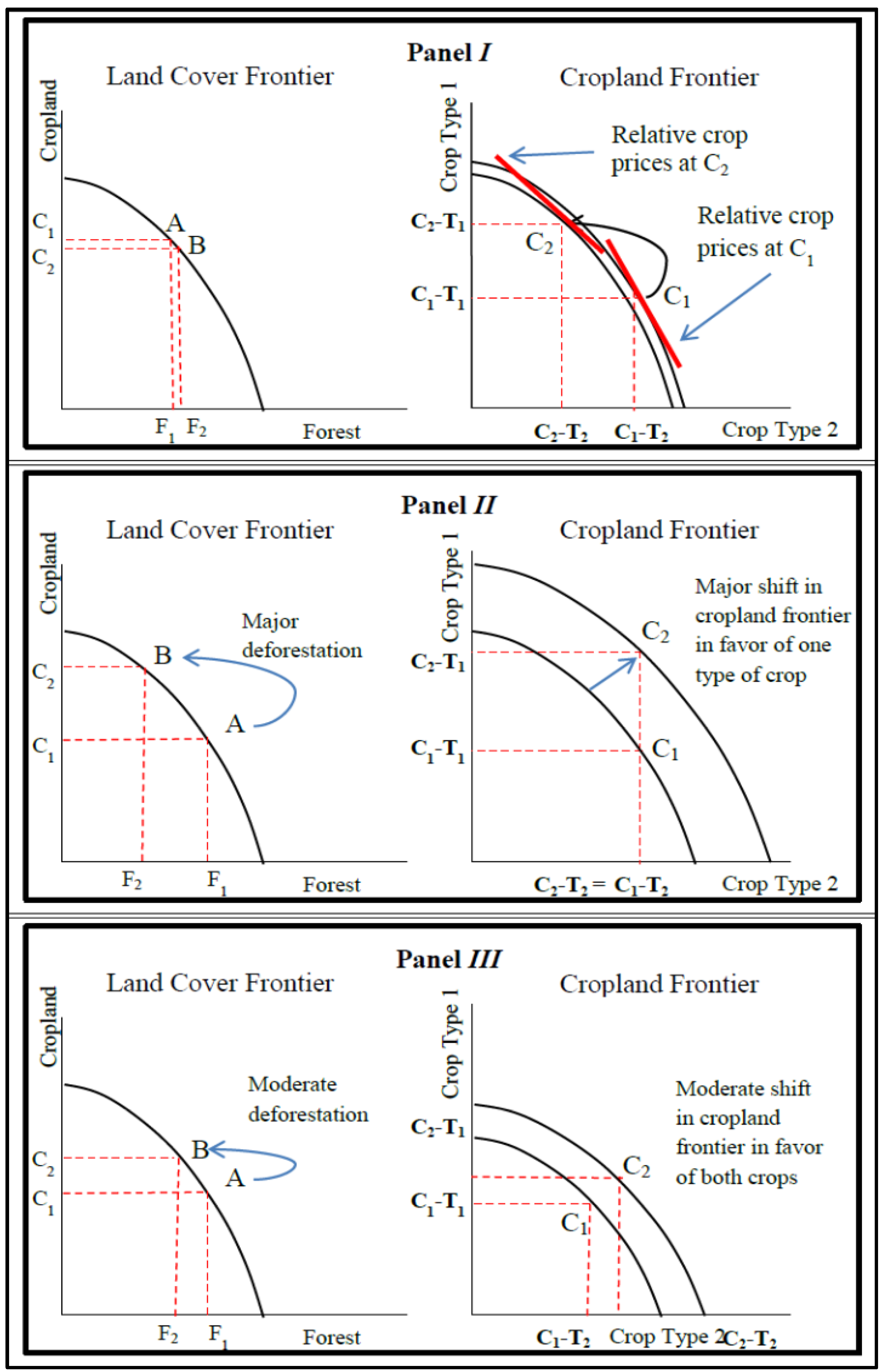
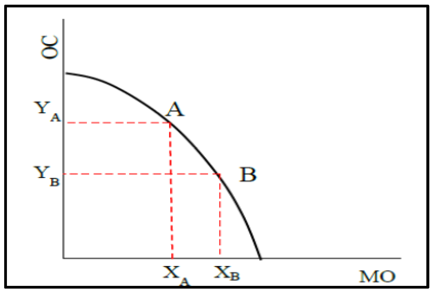
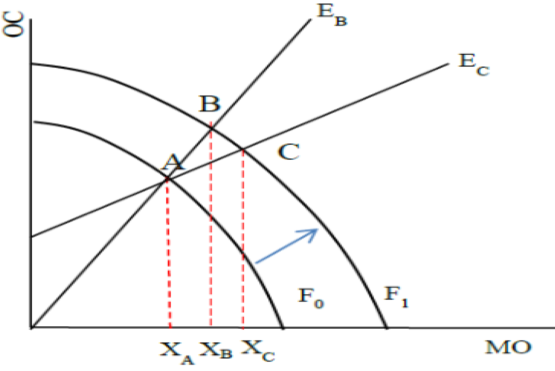
. For example, suppose point A represents the year 2003 (one year before biofuel boom) and point B represents 2010. Then ATE = −0.86 for the USA economy between 2003 and 2010. If we change the base to 2002 then ATE = −0.76 and if we change the end year to 2009 then ATE = −0.67. Note that in calculating these values we dropped the term Applsci 03 00014 i002 from the above formula because XB were equal YB in recent years. All of these numbers are indeed around ETL2 = −0.75 used in the latest versions of GTAP-BIO developed by Taheripour et al. [17] and Tyner et al. [18]. We considered this value of ETL2 as the highest rate of land transformation for the cropland cover. The cropland transformation elasticities of other regions are tuned with respect to this benchmark. To accomplish this task the same high value of −0.75 is assigned to the ETL2 for EU, Russia, and Oth_CEE_CIS regions, which observed limited or no expansion in their cropland and moved their existing cropland to MO crops since 2004. On the other hand, for those regions which experienced no major expansion in their cropland area and had no significant changes in their land allocation among crops, we assigned a low value of −0.25 to their ETL2 rate. Several regions including Canada, C_C_Amer, Oth_Europe, MEAS_NAfr, and Oceania fall in this group.
Figure 8. Moving towards MO crop without cropland expansion.
Applsci 03 00014 g008
Finally, a test is developed to decide about the size of ETL2 for other countries which experienced expansion in their cropland and observed changes in their cropland allocation among the MO and OC crops. The test which is explained in Appendix C determines the sources of changes in the area of MO crops in each region over time. The area of MO crop in each region could change due to two sources. It can change either due to expansion in cropland or a combination of expansion in cropland and switching from production of OC to MO crops. In each region, if the expansion occurred only due to cropland expansion, then a limited value of −0.25 is assigned to ETL2 of that region, otherwise a value of −0.5 is used. A full set of new regional ETL2 is presented in Table 1.

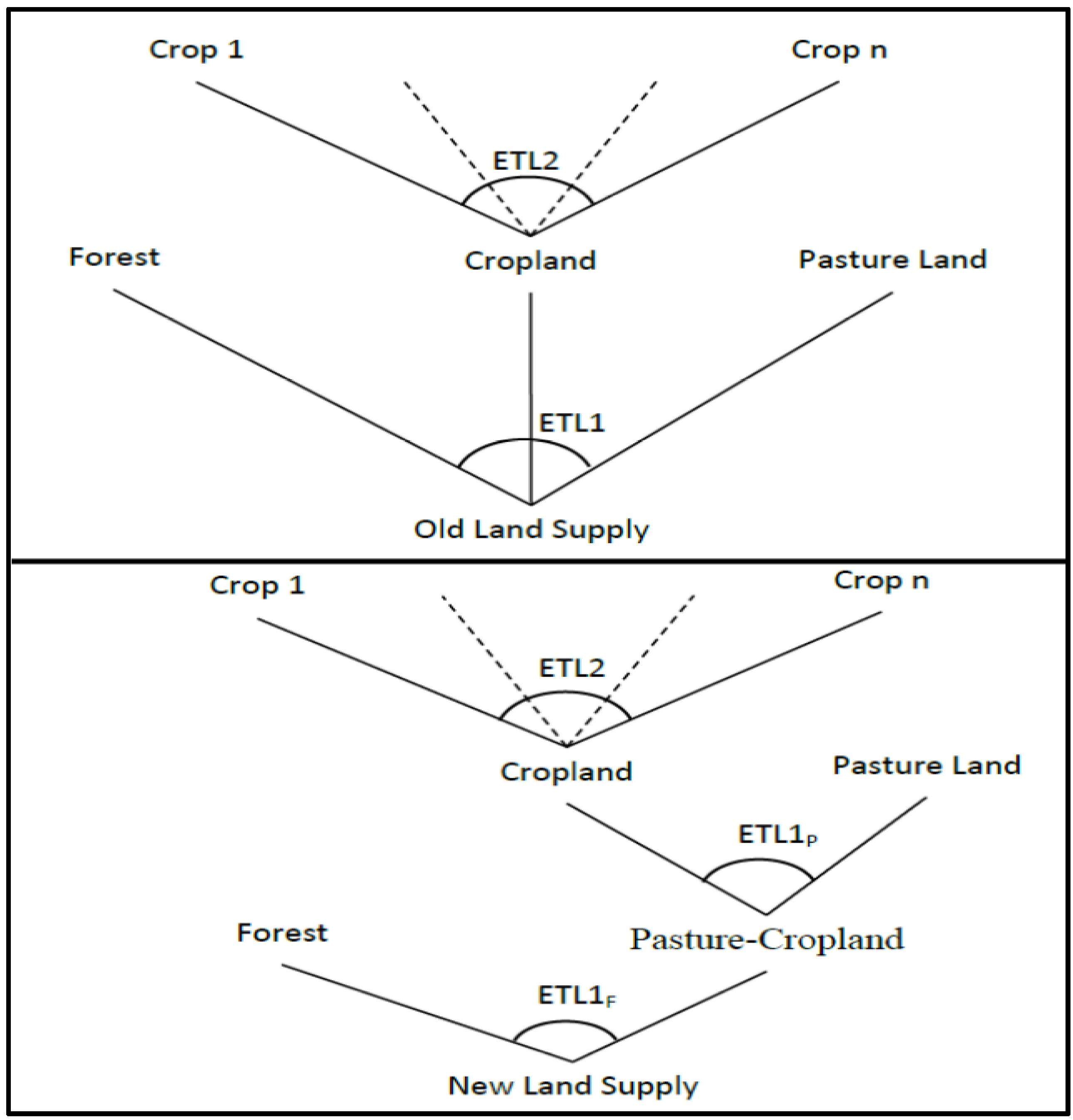
2.3. Change in the Land Cover Nesting Structure

The GTAP-BIO model divides the managed land cover of each region into three broad land categories of cropland, forest, and pasture by AEZ. Cropland denotes existing cultivated land. Managed forest represents all types of forests, and pastureland covers all types of range, grassland, and pasture. Pasture does not include shrubland, which cannot be converted to cropland in GTAP. In this model land can move from one type to another type subject to economic and biophysical constraints. For example, a low productivity pasture will not be converted to cropland when a more suitable land is available for conversion. The supply of and demand for land are modeled at the AEZ level. The derived demands for cropland, forest and pasture are determined from the production functions of crop, forest, and livestock sectors. The land supply side of the model represents a land allocation CET process. The implemented land supply structure of the earlier versions of the GTAP-BIO model put forest, pasture, and cropland in one nest and assumed that forest and pasture land can be converted to crop land with identical rates of land transformation elasticities. This implies that land can be converted from forest and pasture to cropland with equal ease and/or economic opportunity cost. In the real world often it is not as easy or inexpensive to convert forest to cropland as pasture. For example, farmers frequently switch back and forth from pasture and grassland to crop production and vice versa in the Northern Plains regions of the USA (including parts of Iowa, Minnesota, North Dakota, South Dakota and Montana) [20] where converting grasslands to crop production and vice versa is not costly. However, transforming managed forests to cropland is not a common practice. In general, per hectare cost of converting one type of land to another type is equal to the difference in their present values per hectare [21], the value of each type of land is equal to the net present value of its future annual net return/rent, and the net present value of land can evaluated by its annual rent over a discount rate. Gurgel et al. [21] have shown that in general pasture land rent is higher than forest land rent, and both of these land rents are smaller than cropland rent across the world except in a few places. This means that the net costs of converting pasture land to crop production should be less than the net costs of converting forest to cropland. Putting forest, pasture, and cropland in the same nest ignores this important fact.
To remove this deficiency, we created a new land supply nesting structure, shown in the bottom panel of Figure 1, which has cropland and pasture in one nest and the substitution between forest and the combined “pasture–cropland” in the second nest. In this paper we use the notation “pasture–cropland” for the combination of pasture and cropland in the land supply tree. We continue to use the notation “cropland pasture” for low productivity cropland which has been cultivated in past but is not under crop production at present. In the new nesting structure parameter ETL1F shows the land transformation rate between forest and combined pasture–cropland, parameter ETL1P indicates the land transformation rate between cropland and pasture land, and parameter ETL2 represents the rate of land transformation among cropping activities as usual.
To take into account the fact that converting pasture land to cropland is easier and/or less costly than converting forest to cropland, it is assumed that in each region the value of ETL1P is α percent larger than the value of ETL1F. Note that, in the absolute term, the higher the value of land transformation elasticity the lower the economic cost of land transformation. In addition, to preserve the tuned regional ETL1 values presented in Table 1, it is assumed that in each region values of ETL1F and ETL1P deviate from the value of ETL1 of that region by plus and minus β, respectively. Under these assumptions it is straight forward to show that: β= α/(200 + α). In this paper we assumed that ETL1P is 20% larger than ETL1F to take into account the fact that converting forest to cropland is more costly than converting pasture land to cropland. Given these assumptions the regional values for ETL1F and ETL1P are obtained from the regional values of ETL1 presented in Table 1. The calculated values for these land transformation values are presented in Table 2.
Table 2. Tuned regional land cover transformation elasticities.
RegionsRank in land cover changeTuned ETL1Tuned ETL1FTuned ETL1PTuned ETL2
Oth_EuropeVery Low−0.02−0.018−0.0218−0.25
Oceania−0.02−0.018−0.0218−0.25
CAN−0.02−0.018−0.0218−0.25
USA−0.02−0.018−0.0218−0.75
MEAS_NAfr−0.02−0.018−0.0218−0.25
Oth_CEE_CIS−0.02−0.018−0.0218−0.75
C_C_Amer−0.02−0.018−0.0218−0.25
EU27−0.02−0.018−0.0218−0.75
INDIALow−0.1−0.0909−0.1091−0.25
R_S_Asia−0.1−0.0909−0.1091−0.25
RussiaHigh−0.2−0.1818−0.2182−0.75
JAPAN−0.2−0.1818−0.2182−0.5
CHIHKG−0.2−0.1818−0.2182−0.25
E_Asia−0.2−0.1818−0.2182−0.5
BRAZILVery High−0.3−0.2727−0.3273−0.5
R_SE_Asia−0.3−0.2727−0.3273−0.5
Mala_Indo−0.3−0.2727−0.3273−0.25
S_o_Amer−0.3−0.2727−0.3273−0.25
S_S_AFR−0.3−0.2727−0.3273−0.5

3. Results and Discussion

3.1. Land Use Impacts of USA Ethanol Mandate

Several studies have used the GTAP-BIO model which operates based on a land supply tree with a one-nest land cover structure and implements uniform land transformation elasticity values of ETL1 = −0.2 and ETL2 = −0.5 (or recently ETL2 = −0.75) to evaluate the land use impacts of the USA ethanol mandate. The results from these studies indicate that around 50 percent of the expansion in global cropland due to USA ethanol occurs in the USA and that much of that is forest. The following experiments show that moving from this set up to a new GTAP-BIO model which operates based on a land supply tree with a two-nest land cover structure and implements regional land transformation elasticities obtained from regional-historical observations could entirely alter this picture To analyze the impacts of this transition on estimates of induced land use changes due to USA ethanol production the following four experiments are designed and simulated:
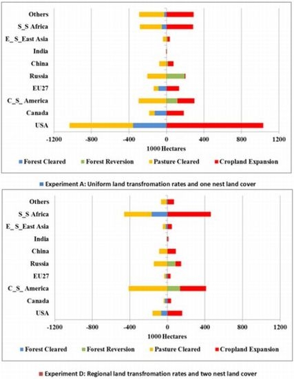
  • Experiment A. An increase in corn ethanol production from its 2004 level (3.41 billion gallons [BG]) to 15 BG, using a land supply tree including a one-nest land cover structure with uniform land transformation rates of ETL1=−0.2 and ETL2=−0.75 across the world.
  • Experiment B. An increase in corn ethanol production from its 2004 level (3.41 billion gallons [BG]) to 15 BG, using a land supply tree including a one-nest land cover structure with regional land transformation rates presented in Table 1.
  • Experiment C. An increase in corn ethanol production from its 2004 level (3.41 billion gallons [BG]) to 15 BG, using a land supply tree including a two-nest land cover structure with uniform land transformation rates of ETL1 = −0.2 and ETL2 = −0.75 across the world while we assume in each region ETL1P is 20% larger than ETL1F.
  • Experiment D. An increase in corn ethanol production from its 2004 level (3.41 billion gallons [BG]) to 15 BG, using a land supply tree including a two-nest land cover structure with regional land transformation rates presented in Table 2.
To implement these experiments the GTAP-BIO modeling framework used in Tyner et al. [18] is modified to handle the new land supply nesting structure with regional land transformation elasticities. The land use consequences of the first two experiments A and B are presented and compared in Table 3.
Table 3. Induced land use changes due to USA ethanol mandate with one-nest land cover: Uniform versus regional land transformation rates (figures are in 1000 hectares).
RegionsExperiment A: Uniform land transformation rates of ETL1 = −0.2 and ETL2 = −0.75Experiment B: Regional land transformation rates Presented in Table 1
ForestCroplandPastureForestCroplandPasture
USA−357.41033.3−675.8−91.6155.7−64.1
EU27−85.8136.2−50.4−21.233.6−12.5
BRAZIL−3.691.6−88.021.7152.1−173.8
CAN−123.9184.5−60.6−29.441.0−11.7
JAPAN−3.03.5−0.5−5.35.30.0
CHIHKG17.159.4−76.4−13.289.7−76.5
INDIA−2.25.2−3.0−7.410.7−3.3
C_C_Amer34.822.3−57.11.85.3−7.0
S_o_Amer85.867.1−152.945.5111.8−157.3
E_Asia4.30.8−5.12.21.5−3.7
Mala_Indo8.2−4.6−3.61.41.6−3.0
R_SE_Asia2.52.8−5.3−12.314.4−2.1
R_S_Asia−2.024.9−23.0−3.223.5−20.3
Russia194.39.5−203.994.352.1−146.4
Oth_CEE_CIS−22.6110.3−87.7−8.827.5−18.8
Oth_Europe−0.11.7−1.6−0.30.4−0.1
MEAS_NAfr−0.189.6−89.5−0.121.1−21.0
S_S_AFR−48.7284.3−235.7−213.9470.5−256.6
Oceania−0.989.2−88.3−0.916.8−15.9
Total−303.32211.7−1908.4−240.61234.6−994.0
Cropland Pasture
USA−1218.6−1793.7
Brazil−271.5−221.2
Table 3 indicates that experiment B with the new regional land transformation rates projects an expansion in global cropland by about 1.2 MH, which is significantly smaller (by 44%) than the corresponding figure obtained from experiment A with uniform land transformation values. The geographical distribution of induced cropland expansion indicates the share of USA changes from 47% to 13% when we use the regional parameters. We checked to see if there was a significant yield increase due to intensification from the CET parameter change, and found that the changes were small in all regions. The shares of EU27, Canada, also fall significantly. On the other hand the shares of several other regions (in particular, S_S_AFR and S_o_Amer) go up.
Incorporation of the regional land transformation elasticities increases the share of forest in expanded cropland from 13.7% to 19.5% at the global scale. On the other hand, in the USA, cropland pasture conversion increases significantly, by more than 0.5 MH (or 47%).
Table 4. Induced land use changes due to USA ethanol mandate with two-nest land cover: Uniform versus regional land transformation rates (figures are in 1000 hectares).
RegionsExperiment C: Uniform land transformation rates of ETL1F = −0.1818, ETL1P = −0.2182, and ETL2 = −0.75Experiment D: Regional land transformation rates Presented in Table 2
ForestCroplandPastureForestCroplandPasture
USA−243.01055.9−812.9−64.8157.4−92.7
EU27−73.3137.2−64.0−14.733.6−18.8
BRAZIL45.2101.0−146.362.5156.7−219.2
CAN−110.4176.1−65.6−25.440.1−14.8
JAPAN−2.93.5−0.6−5.05.2−0.1
CHIHKG21.960.2−82.2−1.788.6−86.8
INDIA−2.55.7−3.2−7.010.5−3.5
C_C_Amer38.122.4−60.54.55.4−9.9
S_o_Amer100.272.1−172.368.9114.4−183.3
E_Asia4.00.9−5.02.21.5−3.8
Mala_Indo7.2−3.9−3.30.92.1−3.0
R_SE_Asia2.03.1−5.2−11.814.4−2.5
R_S_Asia−1.926.2−24.2−3.124.7−21.6
Russia176.118.5−194.787.358.0−145.3
Oth_CEE_CIS−21.3114.8−93.5−7.428.8−21.4
Oth_Europe−0.31.9−1.7−0.20.4−0.2
MEAS_NAfr0.592.8−93.30.221.8−21.9
S_S_AFR−14.8273.0−258.2−167.1461.8−294.7
Oceania−0.193.6−93.5−0.517.9−17.3
Total−74.92255.1−2180.2−82.41243.2−1160.8
Cropland Pasture
USA −1195.4 −1788.5
Brazil 213.4 −213.9
Consider now the difference between the results obtained from experiments A (in Table 3) and C (in Table 4). Both experiments are built based on uniform land transformation elasticities, but the former uses a one-nest land cover and the latter uses a two-nest land cover with different values for pasture–cropland and the combination of pasture–cropland and forest. These two experiments project very similar patterns for cropland expansion; however the two-nest model estimates a significantly smaller share for forest in expanded cropland. The share of forest in global expanded cropland decreases from 14% to 3%. This indicates that using a two-nest land cover only affects the share of forest in expanded cropland due to ethanol production.
We now move to experiment D (Table 4) which includes both regional land transformation elasticities and a two-nest land cover structure. Compared to experiment C, this experiment projects a significantly smaller cropland expansion, by about 45%. And compared to experiment B, it projects a major drop in the share of forest in cropland expansion, 20% in experiment B versus 7% in experiment D. Finally, in comparing experiments A and D one can see that using a two-nest structure with regional land transformation elasticities reduces the magnitude of cropland expansion by about 45%, and decreases the share of forest in cropland expansion to 7%.
In conclusion, these analyses show that moving towards regional land transformation elasticities reduces the magnitude of land conversion and using the two-nest land cover nesting structure decreases the share of forest in land conversion. The combination of these two changes will contribute to lower estimations for induced land use emissions due to ethanol production.
Consider now Figure 9 which compares the regional expansions in cropland areas obtained from experiments A and D. This figure shows that the geographical distribution of cropland expansion obtained from these two experiments are very different. Comparing Figure 7 and Figure 9, it is clear that experiment D does a much better job of representing the actual land use changes seen over the past six years. There are still differences, but the new model which uses a two-nest land cover and implements regional land transformation elasticities represents a significant improvement. And while the ethanol shock is just one of many actual shocks, the land use changes likely play out in a similar way to the idealized case with all shocks present.
Figure 9. Cropland expansion due to USA ethanol mandate based on experiments A and D.
Applsci 03 00014 g009
Finally, compare Figure 10 and Figure 11 which compare induced land use changes by land types for experiments A and D. Figure 10 shows that in experiment A the ethanol expansion causes deforestation (by 0.36 MH) and conversion of pasture land (by 0.68 MH) in the US. But Figure 11, which represents the results of experiment D, results in much lower USA land cover change due to ethanol production (about 0.09 MH deforestations, 0.06 MH pasture conversions, and 0.15 MH expansions in cropland). In addition, these figures show that the model with the new modifications projects larger land conversions in Central and South America and Sub Saharan Africa.
Figure 10. Changes in global land cover in experiment A with original uniform land transformation elasticities.
Applsci 03 00014 g010
Figure 11. Changes in global land cover in experiment D with regional tuned land transformation elasticities.
Applsci 03 00014 g011

3.2. Land Use Emissions Due to Land Use Impacts of USA Ethanol Mandate

To measure land use emissions for the cases developed in this paper we rely on the land use emissions factors reported for a 30-year time horizon by Plevin et al. [22]. These authors provided a model which measures carbon fluxes due to land use changes induced by biofuel production at the AEZ level at a global scale. The estimated land emissions for the experiments A and D are about 20.3 g CO2eMJ−1 and 13.3 g CO2eMJ−1. With these figures we can conclude that using a two-nest land cover structure and applying regional land transformation rates jointly reduce the calculated land use emissions by about 18%, which is significantly smaller than the reduction in the estimated harvested area. Part of the reason for this difference is the fact that these emission factors include cropland pasture, and there is more cropland pasture conversion in experiment D than experiment A.

4. Conclusions

Previous versions of the GTAP-BIO model assume uniform values for the land transformation elasticities for all regions worldwide. They also put forest, pasture and cropland in one nest and assume forest and pasture land can be converted to cropland with identical land transformation elasticities. In prior work there was not much land use change globally that could be used to calibrate GTAP parameters, but in the past decade there has been substantial land cover change corresponding to the period of the biofuels boom. The actual land use changes have varied significantly from one region to another during the past two decades across the world. In addition, in real world converting forest to cropland is more costly than converting pasture to cropland.
While we recognize that the CET parameter is not the only factor driving the extent and location of land use change, it is one of the important parameters and one that can easily be varied by region. This paper reviews changes in global cropland and indicates that during the past two decades countries around the world have followed different land allocation patterns in the face of changes in markets for crop products. While some regions have expanded their cropland significantly, other regions mainly reallocated their existing cropland among alternative crops. This suggests that the land transformation rates vary across the world. Based on these observations, uniform land transformation elasticities are modified. In addition, the land cover nesting structure of the land supply tree is modified. In the new land supply tree cropland and pasture are in one nest, and the combination of these two types of land cover with forest are in another nest. Then the land use consequences of the USA ethanol mandate are evaluated with these model and parameter changes.
The implemented experiments show that moving towards regional land transformation elasticities reduces the magnitude of land conversion, and using the two-nest land cover nesting structure decreases the share of forest in land conversion. The combination of these two changes reduces the magnitude of cropland expansion by 45%, and decreases the share of forest in cropland expansion to 7%. The estimated land use emissions due to ethanol production falls by 18%. In addition, about 0.5 MH more cropland pasture will be converted to cropland due to these two modifications.

Acknowledgments

Partial funding for this research was provided by Office of Energy Products and New Uses, U.S. Department of Agriculture, by the National Institute of Food And Agriculture, U.S. Department of Agriculture, and also by the National Biodiesel Board.

Appendix A

Table A1. List of crop categories and their members.
Name of crop in FAOMAP to 10 cropsName of crop in FAOMAP to 10 crops
Agave Fibres NesFibersCoconutsOil_Seeds
Alfalfa for forage and silageAnimal_FeedCoffee, greenOthers
Almonds, with shellVe_Fr_FoodCow peas, dryVe_Fr_Food
Anise, badian, fennel, corian.Animal_FeedCranberriesVe_Fr_Food
ApplesVe_Fr_FoodCucumbers and gherkinsVe_Fr_Food
ApricotsVe_Fr_FoodCurrantsVe_Fr_Food
ArecanutsVe_Fr_FoodDatesVe_Fr_Food
ArtichokesVe_Fr_FoodEggplants (aubergines)Ve_Fr_Food
AsparagusVe_Fr_FoodFibre Crops NesFibers
AvocadosVe_Fr_FoodFigsVe_Fr_Food
Bambara beansVe_Fr_FoodFlax fibre and towFibers
BananasVe_Fr_FoodFonioCgrainNoCorn
BarleyCgrainNoCornforage ProductsAnimal_Feed
Beans, dryVe_Fr_FoodFruit Fresh NesVe_Fr_Food
Beans, greenVe_Fr_FoodFruit, tropical fresh nesVe_Fr_Food
Beets for FodderAnimal_FeedGarlicVe_Fr_Food
Berries NesVe_Fr_FoodGingerOthers
BlueberriesVe_Fr_FoodGooseberriesVe_Fr_Food
Brazil nuts, with shellVe_Fr_FoodGrapefruit (inc. pomelos)Ve_Fr_Food
Broad beans, horse beans, dryVe_Fr_FoodGrapesVe_Fr_Food
BuckwheatCgrainNoCornGrasses Nes for forage;SilAnimal_Feed
Cabbage for FodderAnimal_FeedGreen Oilseeds for SilageAnimal_Feed
Cabbages and other brassicasVe_Fr_FoodGroundnuts, with shellOil_Seeds
Canary seedCgrainNoCornHazelnuts, with shellVe_Fr_Food
CarobsVe_Fr_FoodHemp Tow WasteFibers
Carrots and turnipsVe_Fr_FoodHempseedOil_Seeds
Carrots for FodderAnimal_FeedHopsOthers
Cashew nuts, with shellVe_Fr_FoodJojoba SeedsOil_Seeds
CashewappleVe_Fr_FoodJuteFibers
CassavaVe_Fr_FoodKapok FruitFibers
Castor oil seedOil_SeedsKarite Nuts (Sheanuts)Oil_Seeds
Cauliflowers and broccoliVe_Fr_FoodKiwi fruitVe_Fr_Food
Cereals, nesCgrainNoCornKolanutsVe_Fr_Food
CherriesVe_Fr_FoodLeeks, other alliaceous vegVe_Fr_Food
ChestnutsVe_Fr_FoodLeguminous for SilageAnimal_Feed
Chick peasVe_Fr_FoodLeguminous vegetables, nesAnimal_Feed
Chicory rootsVe_Fr_FoodLemons and limesVe_Fr_Food
Chillies and peppers, dryVe_Fr_FoodLentilsVe_Fr_Food
Chillies and peppers, greenVe_Fr_FoodLettuce and chicoryVe_Fr_Food
Cinnamon (canella)OthersLinseedOil_Seeds
Citrus fruit, nesVe_Fr_FoodLupinsAnimal_Feed
Clover for forage and silageAnimal_FeedMaizeGrain_Maize
ClovesAnimal_FeedMaize for forage and silageAnimal_Feed
Cocoa beansOthersMaize, greenVe_Fr_Food
Mangoes, mangosteens, guavasVe_Fr_FoodRamieFibers
Manila Fibre (Abaca)FibersRapeseedOil_Seeds
MatéAnimal_FeedRaspberriesVe_Fr_Food
MelonseedOil_SeedsRice, paddyPaddy_Rice
MilletCgrainNoCornRoots and Tubers, nesOthers
Mixed grainCgrainNoCornRyeCgrainNoCorn
Mushrooms and trufflesOthersRye grass for forage & silageAnimal_Feed
Mustard seedOil_SeedsSafflower seedOil_Seeds
Natural rubberOthersSeed cottonFibers
Nutmeg, mace and cardamomsOthersSesame seedOil_Seeds
Nuts, nesVe_Fr_FoodSisalFibers
OatsCgrainNoCornSorghumCgrainNoCorn
Oil palm fruitOil_SeedsSorghum for forage and silageAnimal_Feed
Oilseeds, NesOil_SeedsSour cherriesVe_Fr_Food
OkraVe_Fr_FoodSoybeansSoybeans
OlivesOil_SeedsSpices, nesOthers
Onions (inc. shallots), greenVe_Fr_FoodSpinachVe_Fr_Food
Onions, dryVe_Fr_FoodStone fruit, nesVe_Fr_Food
OrangesVe_Fr_FoodStrawberriesVe_Fr_Food
Other BastfibresFibersString beansVe_Fr_Food
Other melons (inc.cantaloupes)Ve_Fr_FoodSugar beetOthers
PapayasVe_Fr_FoodSugar caneOthers
Peaches and nectarinesVe_Fr_FoodSugar crops, nesOthers
PearsVe_Fr_FoodSunflower seedOil_Seeds
Peas, dryVe_Fr_FoodSwedes for FodderAnimal_Feed
Peas, greenVe_Fr_FoodSweet potatoesVe_Fr_Food
Pepper (Piper spp.)OthersTallowtree SeedsOil_Seeds
PeppermintOthersTangerines, mandarins, clem.Ve_Fr_Food
PersimmonsVe_Fr_FoodTaro (cocoyam)Ve_Fr_Food
Pigeon peasVe_Fr_FoodTeaOthers
PineapplesVe_Fr_FoodTea NesOthers
PistachiosVe_Fr_FoodTobacco, unmanufacturedOthers
PlantainsVe_Fr_FoodTomatoesVe_Fr_Food
Plums and sloesVe_Fr_FoodTriticaleCgrainNoCorn
Pome fruit, nesVe_Fr_FoodTung NutsOil_Seeds
PopcornCgrainNoCornTurnips for FodderAnimal_Feed
Poppy seedOil_SeedsVanillaOthers
PotatoesVe_Fr_FoodVegetables fresh nesVe_Fr_Food
Pulses, nesVe_Fr_FoodVegetables Roots FodderAnimal_Feed
Pumpkins for FodderVe_Fr_FoodVetchesOthers
Pumpkins, squash and gourdsVe_Fr_FoodWalnuts, with shellVe_Fr_Food
Pyrethrum, DriedAnimal_FeedWatermelonsVe_Fr_Food
QuincesVe_Fr_FoodWheatWheat
QuinoaCgrainNoCornYamsVe_Fr_Food
Yautia (cocoyam)Ve_Fr_Food

Appendix B

Table B1. List of regions and their members.
RegionDescriptionCorresponding Countries in GTAP
USAUnited StatesUsa
EU27European Union 27aut, bel, bgr, cyp, cze, deu, dnk, esp, est, fin, fra, gbr, grc, hun, irl, ita, ltu, lux, lva, mlt, nld, pol, prt, rom, svk, svn, swe
BRAZILBrazilBra
CANCanadaCan
JAPANJapanJpn
CHIHKGChina and Hong Kongchn, hkg
INDIAIndiaInd
C_C_AmerCentral and Caribbean Americasmex, xna, xca, xfa, xcb
S_o_AmerSouth and Other Americascol, per, ven, xap, arg, chl, ury, xsm
E_AsiaEast Asiakor, twn, xea
Mala_Indo Malaysia and Indonesiaind, mys
R_SE_AsiaRest of South East Asiaphl, sgp, tha, vnm, xse
R_S_AsiaRest of South Asiabgd, lka, xsa
Russia Russia Rus
Oth_CEE_CIS Other East Europe and Rest of Former Soviet Unionxer, alb, hrv, xsu, tur
R_EuropeRest of European Countriesche, xef
MEAS_NAfrMiddle Eastern and North Africaxme, mar, tun, xnf
S_S_AFRSub Saharan Africabwa, zaf, xsc, mwi, moz, tza, zmb, zwe, xsd, mdg, uga, xss
OceaniaOceania countriesaus, nzl, xoc

Appendix C

A Test to Determine Sources of Expansion in Harvested Area of Maize and Oilseeds (MO)

This appendix provides a simple test to determine the sources of expansion in the harvested areas of MO crops when the harvested area of a region is expanded over time. In such a case the area of MO crops can be expanded either through the expansion in total harvested area or shifting land from OC to MO crop and vice versa. Consider Figure A1 which represents an expansion in a cropland frontier with an upward shift from the initial position of F0 to the new position of F1. Suppose the initial allocation of cropland among OC and MO crops is at point A on the F0 frontier. The allocation of cropland among these two crop categories can be located on any point on the F1 frontier. Consider two possible allocations of B and C. If the economy moves to point B then the line EB represents the expansion path of harvested area in this case. If the economy moves to point C then the line EC represents the expansion path. The line EB shows a monotonic expansion path. In this case the harvested areas of both crops will increase proportionally due to the expansion in total harvested area. This line goes through the origin and has no intercept. In this case no substitution among harvested areas will happen over time. If the economy moves to point C, then the line EC represents a non-monotonic expansion path. In this case the harvested area of MO expands due to both expansion in total harvested area and moving cropland from OC to MO.
Hence, if the expansion path of harvested area in a region represents a monotonic pattern, then one can conclude no substitution among crops occurs. And if the expansion path of harvested area in a region represents a non-monotonic pattern, then substitution among crops over time does happen.
Following this conclusion an expansion path is estimated for each of the regions which experienced expansion in harvested area since 2004. Then for each region, if its expansion path was representing a monotonic pattern a value of −0.25 is assigned to its cropland transformation rate, otherwise a value of −0.5 is used.
Figure C1. Changes in global land over in experiment D.
Applsci 03 00014 g012

References

  1. Houghton, R.A. Revised estimates of the annual net flux of carbon to the atmosphere from changes in land use and land management: 1850–2000. Tellus B 2003, 55, 378–390. [Google Scholar] [CrossRef]
  2. Ramankutty, N.; Foley, J.A. Estimating historical changes in global land cover: Croplands from 1700 to 1992. Global Biogeochem. Cycles 1999, 13, 997–1027. [Google Scholar] [CrossRef]
  3. Global Forest Resource Assessment 2010; Food and Agricultural Organization of the United Nation: Rome, Italy, 2010.
  4. Tokgoz, S.; Elobeid, A.; Fabiosa, J.F.; Hayes, D.J.; Babcock, B.A.; Yu, T.; Dong, F.; Hart, C.E.; Beghin, J.C. Emerging Biofuels: Outlook of Effects on U.S. Grain, Oilseed, and Livestock Markets; Staff Report 07-SR 101; Center for Agricultural and Rural Development: Ames, IA, USA, 2007. [Google Scholar]
  5. Kammen, D.M.; Farrell, A.E.; Plevin, R.J.; Jones, A.D.; Delucchi, M.A.; Nemet, G.F. Energy and Greenhouse Impacts of Biofuels: A Framework for Analysis; Discussion paper 2007–2; Joint Transport Research Centre: Berkeley, CA, USA, 2007. [Google Scholar]
  6. Searchinger, T.; Heimlich, R.; Houghton, R.; Dong, F.; Elobeid, A.; Fabiosa, J.; Tokgoz, S.; Hayes, D.; Yu, T. Use of U.S. Croplands for Biofuels Increases Greenhouse Gases Through Emissions from Land-Use Change. Science 2008, 319, 1238–1240. [Google Scholar] [CrossRef]
  7. Hertel, T.; Golub, A.; Jones, J.; O’Hare, M.; Pelvin, R.; Kammen, D. Effects of USA Maize Ethanol on Global Land Use and Greenhouse Gas Emissions: Estimating Market-Mediated Responses. BioScience 2010, 60, 223–231. [Google Scholar] [CrossRef]
  8. Al-Riffai, P.; Dimaranan, B.; Laborde, D. Global Trade and Environmental Impact Study of the EU Biofuels Mandate; International Food Policy Research Institute: Washington, DC, USA, 2010. [Google Scholar]
  9. EPA, Renewable Fuel Standard Program (RFS2) Regulatory Impact Analysis; United States Environmental Protection Agency: Washington, DC, USA, 2010.
  10. Taheripour, F.; Hertel, T.; Tyner, W.; Bechman, J.; Birur, D. Biofuels and Their By-Products: Global Economic and Environmental Implications. Biomass Bioenergy 2010, 34, 278–289. [Google Scholar] [CrossRef]
  11. Tyner, W.; Taheripour, F.; Zhuang, Q.; Birur, D.; Baldos, U. Land Use Changes and Consequent CO2 Emissions due to USA Corn Ethanol Production: A Comprehensive Analysis; Department of Agricultural Economics: West Lafayette, IN, USA, 2010. [Google Scholar]
  12. Taheripour, F.; Hertel, T.; Tyner, W. Implications of Biofuels Mandates for the Global Livestock Industry: A Computable General Equilibrium Analysis. Agric. Econ. 2011, 42, 325–342. [Google Scholar] [CrossRef]
  13. Laborde, D. Assessing the Land Use Change Consequences of European Biofuels Policies; International Food Policy Research Institute: Washington, DC, USA, 2011. [Google Scholar]
  14. Wicke, B.; Verweij, R.; Meijl, H.; Vuuren, D.; Faaij, A. Indirect Land Use Changes: Review of Existing Models and Strategies for Mitigation. Biofuels 2012, 3, 87–100. [Google Scholar] [CrossRef]
  15. Ahmed, S.; Hertel, T.; Lubowski, R. Calibration of a Land Cover Supply Function Using Transition Probabilities; GTAP Research Memorandum No 12; Center for Global Trade Analysis: West Lafayette, Indiana, USA, 2008. [Google Scholar]
  16. Palatnik, R.; Kan, I.; Rapaport-Rom, M.; Ghermandi, A.; Eboli, F.; Shechter, M. Land Transformation Analysis and Application. Presented at the 14th Annual Conference on Global Economic Analysis. Venice, Italy, June 2011. [Google Scholar]
  17. Taheripour, F.; Tyner, W.; Wang, M. Global Land Use Changes due to the U.S. Cellulosic Biofuel Program Simulated with the GTAP Model; Purdue University, Department of Agricultural Economics: West Lafayette, IN, USA, 2011. [Google Scholar]
  18. Tyner, W.; Taheripour, F.; Golub, A. Calculation of Indirect Land Use Change (ILUC) Values for Low Carbon Fuel Standard (LCSF) Fuel Pathways; Interim report prepared for California Air Resource Board; Purdue University, Department of Agricultural Economics: West Lafayette, IN, USA, 2011. [Google Scholar]
  19. Lubowski, R. Determinants of Land Use Transitions in the United States: Econometrics Analysis of Changes among the Major Land-Use Categories. Ph.D. Thesis, Harvard University, Cambridge, MA, USA, February 2002. [Google Scholar]
  20. USDA, Grassland to Cropland Conversion in the Northern Plains: The Role of Crop Insurance, Commodity, and Disaster Programs; Economic Research Report Number 120; Economic Research Service: Washington, WA, USA, 2011.
  21. Gurgel, A.; Reilly, J.; Paltsev, S. Potential Land Use Implications of a Global Biofuels Industry. J. Agric. Food Ind. Organization 2007, 5. Article 9. [Google Scholar]
  22. Plevin, R.; Gibbs, H.; Duffy, J.; Yui, S.; Yeh, S. Agro-Ecological Zone Emission Factor Model; California Air Resource Board: Sacramento, CA, USA, 2011. [Google Scholar]

