Training for Defense? From Stochastic Traits to Synchrony in Giant Honey Bees (Apis dorsata)

Abstract
:1. Introduction
2. Material and Methods
2.1. Study Site and Experimental Nests

2.2. Video Recording
2.3. Infrared Recording
2.4. Dummy Wasp Stimulation
2.5. Observation Session
2.6. Experimental Sessions
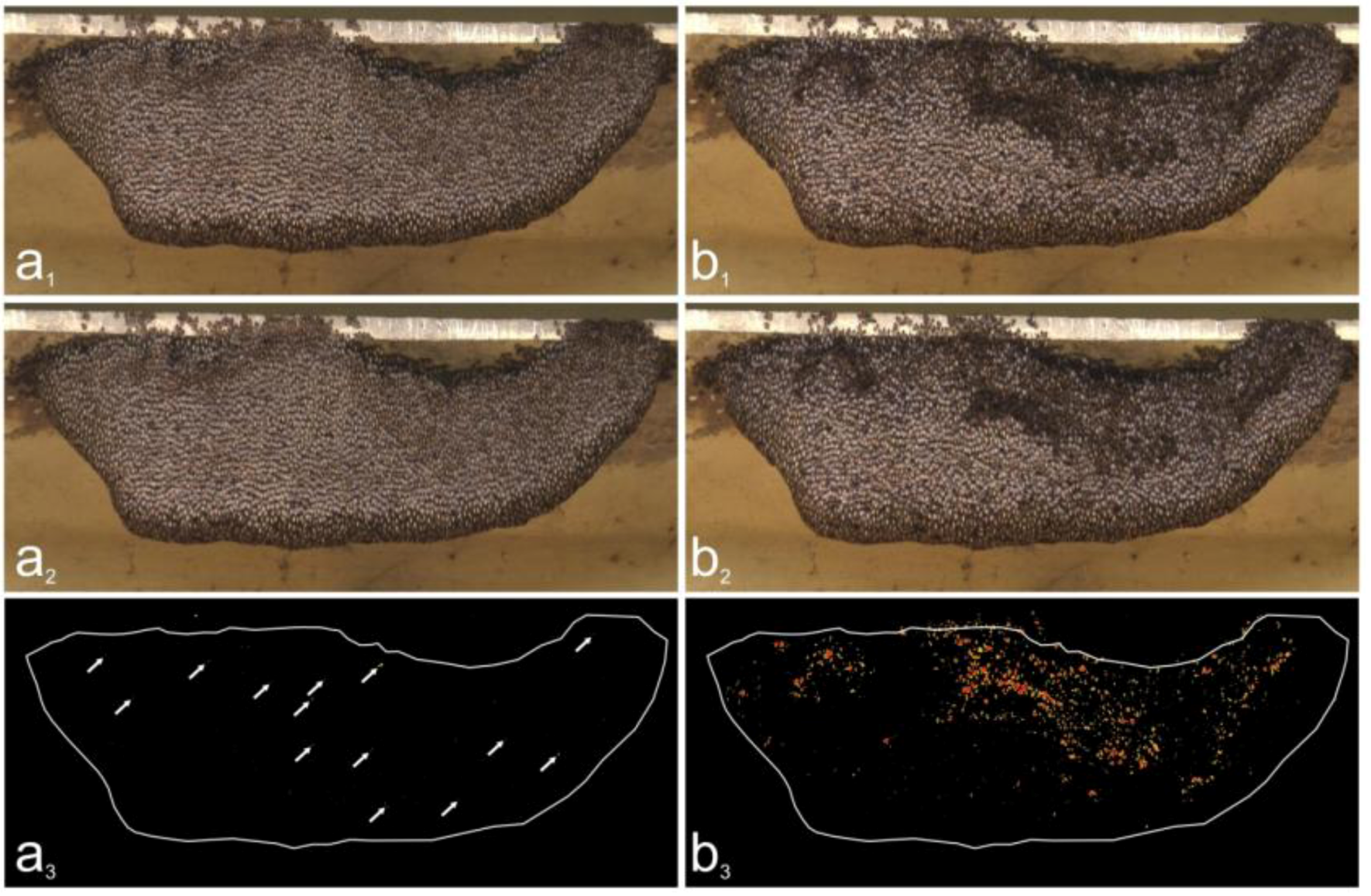
2.7. Assessment of Motion Activities
2.8. Definition of Test Grids
2.9. Assessment of Trigger and Non-trigger Sites
2.10. Assessment of Motion Activities at Trigger Sites

2.11. Identification of Flickering Activity
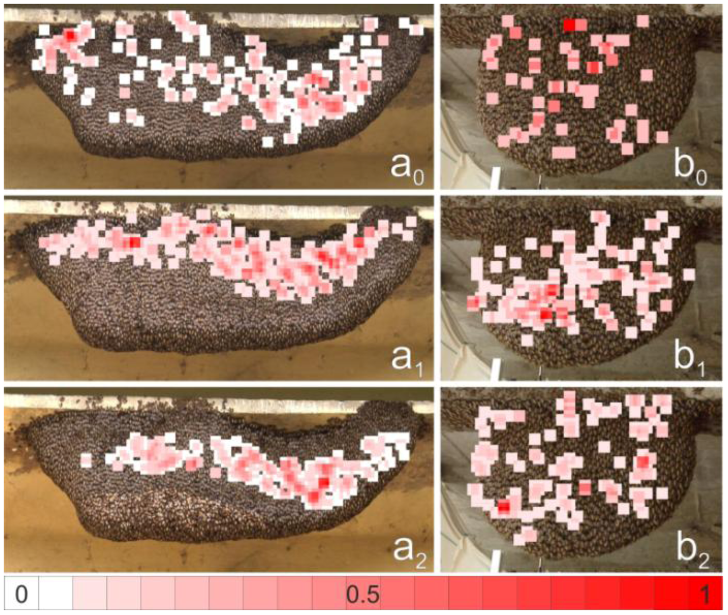
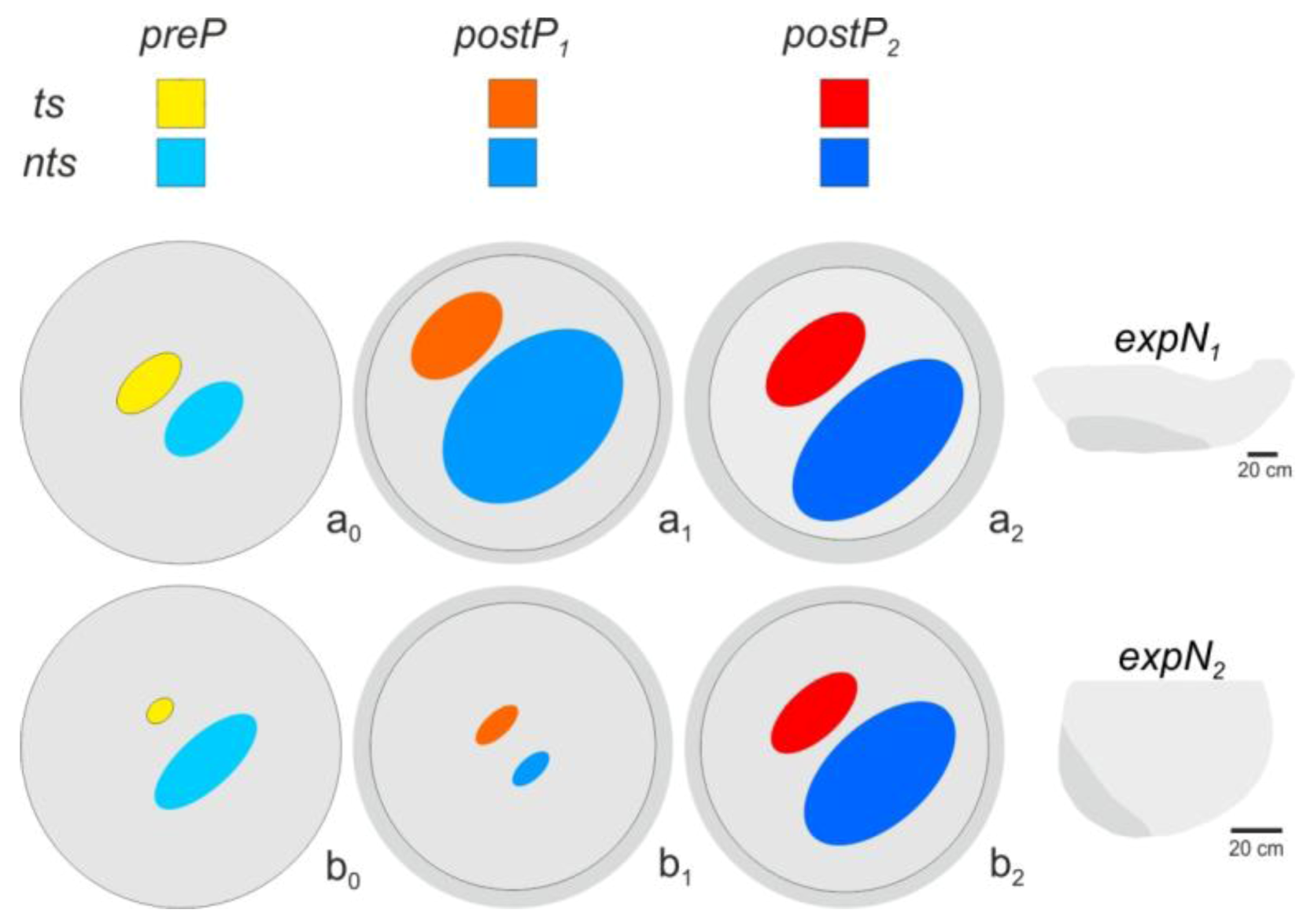
2.12. Spatial Distribution of Trigger Sites of Shimmering Waves
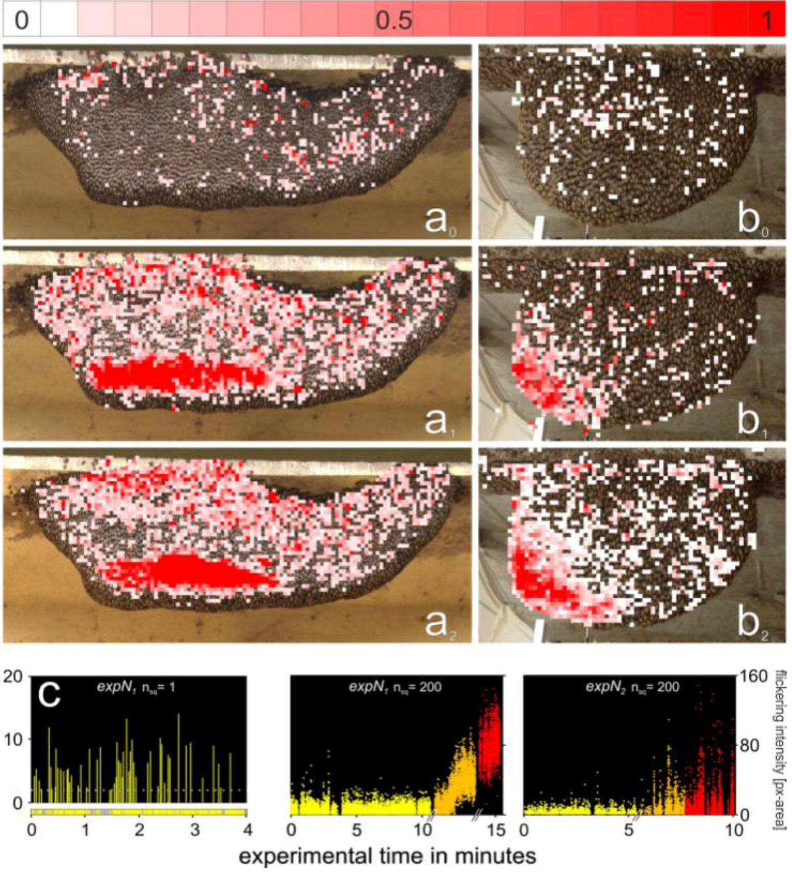
2.13. Assessment of the Spatial Distribution of the Flickering Intensity
3. Results
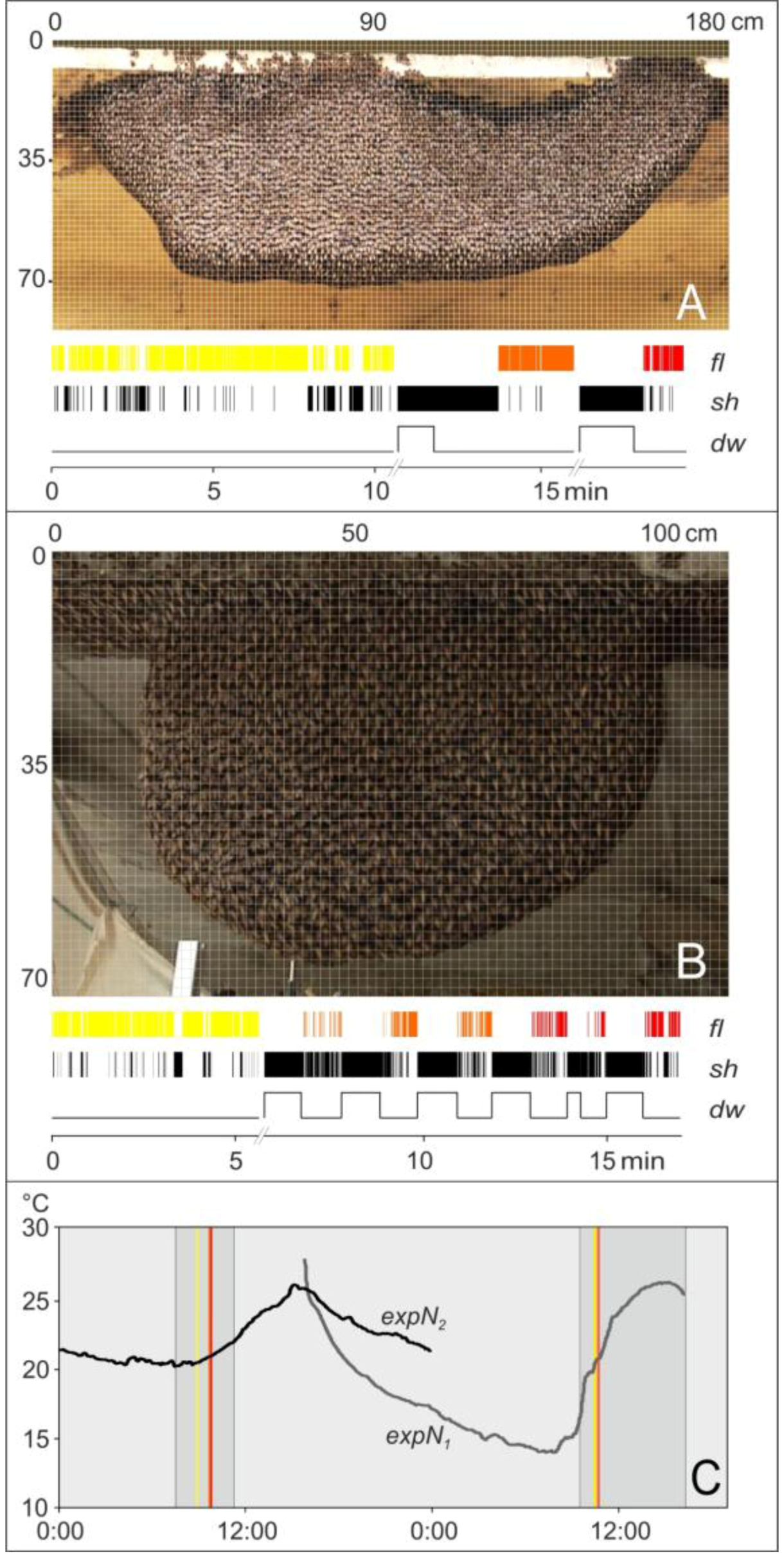
3.1. Observation
3.2. Assessment of Flickering and Shimmering Data in the Experimental Phases

| Nest site | expPhase | Nwaves | Nts | expPhase | relFts+nts | relFts | relFnts |
|---|---|---|---|---|---|---|---|
| expN1 | preP | 36 | 322 | preP | 0.40 | 0.18 | 0.22 |
| P1+postP1 | 26 | 325 | postP1 | 0.86 | 0.28 | 0.58 | |
| P2+postP2 | 13 | 258 | postP2 | 0.88 | 0.33 | 0.55 | |
| expN2 | preP | 11 | 61 | preP | 0.34 | 0.08 | 0.26 |
| P1+postP1 | 27 | 276 | postP1 | 0.24 | 0.13 | 0.11 | |
| P2+postP2 | 17 | 211 | postP2 | 0.73 | 0.26 | 0.47 | |
| Total numbers | 130 | 1453 |
3.3. Spatial Distribution of Trigger Sites of Shimmering Waves
3.4. Assessment of Flickering Activity
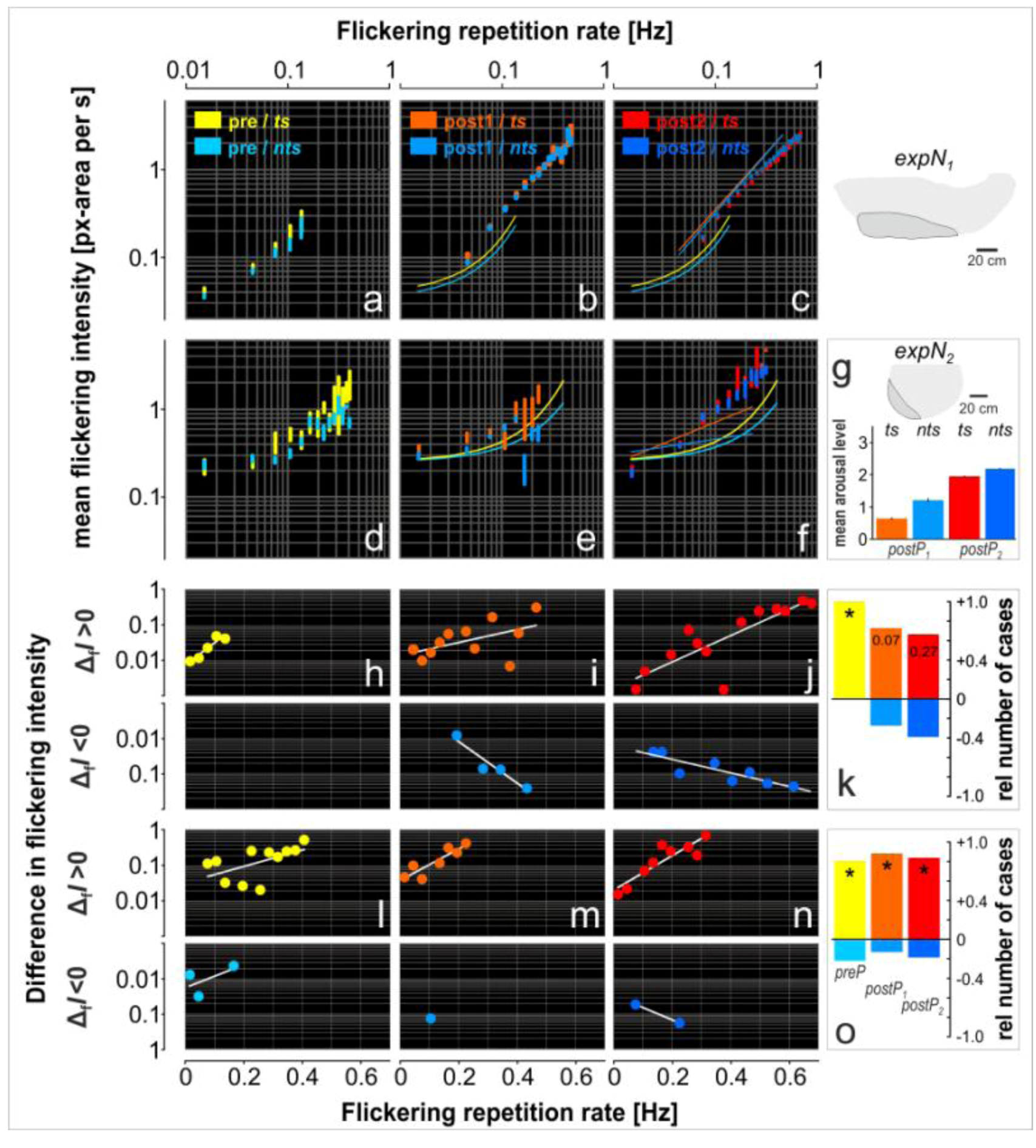
3.5. Rate and Intensity Characteristics of Flickering

| Nest site | expPhase | ts | nts |
|---|---|---|---|
| expN1 | preP | y = 0,0046e19,37x | - |
| R² = 0,8952 | |||
| P1+postP1 | y = 0,0102e5,6643x | y = 0,0035e18,121x | |
| R² = 0,2706 | R² = 0,9126 | ||
| P2+postP2 | y = 0,0016e8,5925x | y = 0,0163e4,383x | |
| R² = 0,6911 | R² = 0,7555 | ||
| expN2 | preP | y = 0,0328e7,1152x | y = 0,0148e-10,05x |
| R² = 0,2964 | R² = 0,3423 | ||
| P1+postP1 | y = 0,0389e13,702x | - | |
| R² = 0,7962 | |||
| P2+postP2 | y = 0,0167e14,98x | y = 0,0281e10,795x | |
| R² = 0,8067 | R² = 1 |
4. Discussion
4.1. Purposes of Flickering in Giant Honey Bees
4.2. Proximate Flickering Hypotheses (Woyke et al. 2004)
4.3. Does the Colony-Intrinsic State induce Diversity in Flickering Activity?
4.4. Ultimate Flickering Hypotheses
4.5. Flickering as a Mass Recruitment Process
5. Conclusions
Supplementary Material
Supplementary Files
Supplementary File 1Acknowledgments
References
- Morse, R.A.; Laigo, F.M. Apis Dorsata in the Philippines; Philippine Association of Entomologists: Laguna, Malaysia, 1969. [Google Scholar]
- Koeniger, N.; Fuchs, S. Zur Kolonieverteidigung der asiatischen Honigbienen. Z. Tierpsychol. 1975, 37, 99–106. [Google Scholar] [CrossRef]
- Seeley, T.D.; Seeley, R.H.; Aratanakul, P. Colony defense strategies of the honeybees in Thailand. Ecol. Monogr. 1982, 52, 43–63. [Google Scholar] [CrossRef]
- Kastberger, G. The Magic Trees of Assam-Documentary Film about the Biology of the Giant Honey Bee Apis dorsata; National Geographic: Margate, FL, USA, 1999. [Google Scholar]
- Kastberger, G.; Sharma, D.K. The predator-prey interaction between blue bearded bee eaters (Nyctyonis athertoni) and Giant Honey Bees (Apis dorsata). Apidologie 2000, 31, 727–736. [Google Scholar] [CrossRef]
- Oldroyd, B.; Wongsiri, S. Asian Honey Bees: Biology, Conservation and Human Interactions; Harvard University Press: Cambridge, UK, 2006. [Google Scholar]
- Kastberger, G.; Weihmann, F.; Hoetzl, T. Self-Assembly Processes in Honeybees: The Phenomenon of Shimmering. In Honeybees of Asian; Hepburn, R., Ed.; Springer: Heidelberg, Germany, 2011a; Volume 1, pp. 397–443. [Google Scholar]
- Seeley, T.D. Honey Bee Ecology: A Study of Adaption in Social Life; Princeton University Press: Princeton, NJ, USA, 1985. [Google Scholar]
- Jones, J.C.; Oldroyd, B.P. Nest thermoregulation in social insects. Adv. Insect Physiol. 2007, 33, 153–191. [Google Scholar]
- Kastberger, G.; Schmelzer, E.; Kranner, I. Social waves in Giant Honey Bees repel hornets. PLoS One 2008, 3, e3141. [Google Scholar] [CrossRef]
- Koeniger, N.; Koeniger, G. Observations and experiments on migration and dance communication of Apis dorsata in Sri Lanka. J. Apic. Res. 1980, 19, 21–34. [Google Scholar]
- Dyer, F.C.; Seeley, T.D. Colony migration in the tropical honey bee Apis dorsata F. (Hymenoptera: Apidae). Insectes Soc. 1994, 41, 129–140. [Google Scholar]
- Neumann, P.; Moritz, R.F.A.; Mautz, D. Colony evaluation is not affected by drifting of drone and worker honeybees (Apis mellifera L.) at a performance testing apiary. Apidologie 2000, 31, 67–69. [Google Scholar]
- Paar, J.; Oldroyd, B.; Kastberger, G. Giant Honey Bees return to their nest sites. Nature 2000, 406, 475. [Google Scholar] [CrossRef]
- Winston, M.L. The Biology of the Honey Bee; Harvard University Press: Cambridge, UK, 1987. [Google Scholar]
- Fuchs, S.; Tautz, J. Colony Defence and Natural Enemies. In Honeybees of Asian; Hepburn, R., Ed.; Springer: Heidelberg, Germany, 2011; Volume 1, pp. 369–395. [Google Scholar]
- Kastberger, G.; Weihmann, F.; Hoetzl, T.; Weiss, S.E.; Maurer, M.; Kranner, I. How to join a wave: Decision-making processes in shimmering behavior of Giant Honey Bees (Apis dorsata). PLoS One 2012. [Google Scholar] [CrossRef]
- Lerchbacher, J.; Weihmann, F.; Hoetzl, T.; Singh, M.M.; Maresch, K.; Kastberger, G. Lay distribution of young Giant Honey Bees (Apis dorsata) within a foster colony. 2012. Unpublished work. [Google Scholar]
- Lindauer, M. Ein Beitrag zur Frage der Arbeitssteilung im Bienenstaat. J. Comp. Physiol. 1952, 34, 299–345. [Google Scholar]
- Huang, Z.Y.; Robinson, G.E. Regulation of honey bee division of labor by colony age demography. Behav.Ecol. Sociobiol. 1996, 39, 147–158. [Google Scholar] [CrossRef]
- Woyke, J.; Wilde, J.; Wilde, M. Temperature correlated dorso-ventral abdomen flipping of Apis laboriosa and Apis dorsata worker bee. Apidologie 2004, 35, 493–502. [Google Scholar] [CrossRef]
- Woyke, J.; Wilde, J.; Wilde, M.; Cervancia, C. Abdomen flipping of Apis dorsata breviligula worker bees correlated with temperature of the nest curtain surface. Apidologie 2006, 37, 501–505. [Google Scholar] [CrossRef]
- Kastberger, G.; Weihmann, F.; Hoetzl, T. Complex social waves of Giant Honey Bees provoked by a dummy wasp support the special-agent hypothesis. Commun. Integr. Biol. 2010, 3, 1–2. [Google Scholar] [CrossRef]
- Thapa, R.; Wongsiri, S. Distinct Fanning Behaviour of two Dwarf Honeybees Apis andreniformis (Smith) and Apis florea (Fab.). In Proceedings of Second International Conference of the Asian Apicultural Association; Yogyakatra, Indonesia, 25–30 July 1994; Sakai, T., Ed.; pp. 344–345.
- Jones, J.C.; Myerscough, M.R.; Graham, S.; Oldroyd, B.P. Honey bee nest thermoregulation: Diversity promotes stability. Science 2004, 305, 402–404. [Google Scholar]
- Dyer, F.C. The biology of the dance language. Annu. Rev. Entomol. 2002, 47, 917–949. [Google Scholar] [CrossRef]
- Towne, W.F. Acoustic and visual cues in the dances of four honey bee species. Behav.Ecol. Sociobiol. 1985, 16, 185–187. [Google Scholar] [CrossRef]
- Schmelzer, E.; Kastberger, G. Special agents trigger social waves in Giant Honey Bees (Apis dorsata). Naturwissenschaften 2009, 96, 1431–1441. [Google Scholar] [CrossRef]
- Kastberger, G.; Winder, O.; Steindl, K. Defence Strategies in the Giant Honey Bees Apis dorsata. In Proceedings of the Deutsche Zoologische Gesellschaft, Osnabrück, Germany, 4–8 June 2001; Volume 94, p. 7.
- Kastberger, G.; Maurer, M.; Weihmann, F.; Ruether, M.; Hoetzl, T.; Kranner, I.; Bischof, H. Stereoscopic motion analysis in densely packed clusters: 3D analysis of the shimmering behavior in Giant Honey Bees. Front. Zool. 2011b. [Google Scholar] [CrossRef]
- Kastberger, G.; Kaefer, H. Cascadic Coordination in Defense Behaviour of the Giant Honey Bee Apis dorsata. In Proceedings of the 27th Göttingen neurobiology conference, Göttingen, Germany, 27–30 May 1999; p. 260.
- Kastberger, G.; Stachl, R. Infrared imaging technology and biological apllications. Behav. Res. Methods Instrum. Comput. 2003, 35, 429–439. [Google Scholar] [CrossRef]
- Waddoup, D.; Weihmann, F.; Singh, M.M.; Hoetzl, T.; Kastberger, G. Homoiothermy in Apis dorsata. Occurrence of convention holes. 2011. Unpublished word. [Google Scholar]
- Butler, C.G.; Fletcher, D.J.C.; Walter, D. Hive entrance finding by honeybees (Apis mellifera) foragers. Anim. Behav. 1970, 18, 78–91. [Google Scholar]
- Free, J.B.; Williams, I.H. Exposure of the Nasonov gland by honeybee (Apis mellifera) collecting water. Behaviour 1970, 37, 286–290. [Google Scholar] [CrossRef]
- Morse, R.A.; Boch, R. Pheromone concert in swarming honeybees (Hymenoptera: Apidae). Ann. Entomol. Soc. Am. 1971, 64, 1414–1417. [Google Scholar]
- Schmidt, J.O.; Slessor, K.N.; Winston, M.L. Roles of Nasonov and queen pheromones in attraction of honeybee swarms. Naturwissenschaften 1993, 80, 573–575. [Google Scholar] [CrossRef]
- Kastberger, G.; Raspotnig, G.; Biswas, S.; Winder, O. Evidence of Nasonov scenting in colony defense of the Giant Honey Bee Apis dorsata. Ethology 1998, 104, 27–37. [Google Scholar]
- Free, J.B.; Williams, I.H. The role of the Nasonov gland pheromone in crop communication by honeybees (Apis mellifera L.). Behaviour, 1972; 41, 314–318. [Google Scholar]
- Tan, K.; Wang, Z.; Li, H.; Yang, S.; Hu, Z.; Kastberger, G.; Oldroyd, B.J. An ‘I see you’ preyepredator signal between the Asian honeybee, Apis cerana, and the hornet, Vespa velutina. Anim. Behav. 2012, 83, 879–882. [Google Scholar] [CrossRef]
- Stabentheiner, A.; Pressl, H.; Papst, T.; Hrassnigg, N.; Crailsheim, K. Endothermic heat production in honeybee winter clusters. J. Exp. Biol. 2002, 206, 353–358. [Google Scholar]
- Vollmann, J.; Stabentheiner, A.; Kovac, H. Die Entwicklung der endothermie bei honigbienen. Mitteilungen Dtsch. Ges. Allg. Angew. Entomol. 2004, 14, 467–470. [Google Scholar]
- Huang, Z.Y.; Robinson, G.E. Social Control of Division of Labor in Honey Bee Colonies. In Information Processing in Social Insects; Detrain, C., Deneubourg, J.L., Pasteels, J.M., Eds.; Birkhäuser Verlag: Basel, Switzerland, 1999; Volume 1, pp. 165–186. [Google Scholar]
- Elekonich, M.M.; Schulz, D.J.; Bloch, G.; Robinson, G.E. Juvenile hormone levels in honey bee (Apis mellifera L.) foragers: Foraging experience and diurnal variation. J. Insect Physiol. 2001, 47, 1119–1125. [Google Scholar]
- Schneider, S.S.; Lewis, L.A. The vibration signal, modulatory communication and the organization of labor in honey bees, Apis mellifera. Apidologie 2004, 35, 117–131. [Google Scholar] [CrossRef]
- Rutz, W.; Gerig, L.; Wille, H.; Lüscher, M. A bioassay for juvenile hormone (JH) effects of insect growth regulators (IGR) on adult worker honeybees. Mitteilungen Schweiz. Entomol. Ges. 1976, 47, 307–313. [Google Scholar]
- Hagenguth, H.; Rembold, H. Identification of juvenile hormone 3 as the only juvenile hormone homolog in all developmental stages of the honey bee. Z. Naturforschung 1978, 33, 847–850. [Google Scholar]
- Fluri, P.; Lüscher, M.; Wille, H.; Gerig, L. Changes in weight of the pharyngeal gland and haemolymph titers of juvenile hormone, protein and vitellogenin in worker honey bees. J. Insect Physiol. 1982, 28, 61–68. [Google Scholar] [CrossRef]
- Robinson, G.E. Regulation of honey bee age polyethism by juvenile hormone. Behav. Ecol. Sociobiol. 1987, 20, 329–338. [Google Scholar] [CrossRef]
- Huang, Z.Y.; Robinson, G.E.; Borst, D.W. Physiological correlates of division of labor among similarly aged honey bees. J. Comp. Physiol. 1994, 174, 731–739. [Google Scholar]
- Breed, M.D. Correlations between aggressiveness and corpora allata volume, social isolation, age and dietary protein in worker honeybees. Insectes Soc. 1983, 30, 482–495. [Google Scholar] [CrossRef]
- Pearce, A.N.; Huang, Z.Y.; Breed, M.D. Juvenile hormone and aggression in honey bees. J. Insect Physiol. 2001, 47, 1243–1247. [Google Scholar] [CrossRef]
- Sasagawa, H.; Sasaki, M.; Okada, I. Experimental Induction of the Division of Labor in Worker Apis mellifera L. by Juvenile Hormone (JH) and its Analog. In Proceedings of 30th International Congress, Apimondia, Nagoya, Japan, 10–16 October 1985; pp. 140–143.
- Beshers, S.N.; Huang, Z.Y.; Oono, Y.; Robinson, G.E. Social inhibition and the regulation of temporal polyethism in honey bees. J. Theor. Biol. 2001, 213, 461–479. [Google Scholar] [CrossRef]
- Couzin, I.D.; Krause, J.; Franks, N.R.; Levin, S.A. Effective leadership and decision-making in animal groups on the move. Nature 2005, 433, 513–516. [Google Scholar]
- Jaffe, K.; Howse, P.E. The mass recruitment system of the leaf cutting ant, Atta cephalotes (L.). Anim. Behav. 1979, 27, 930–939. [Google Scholar]
- De Biseau, J.C.; Deneubourg, J.L.; Pasteels, J.M. Collective flexibility during mass recruitment in the ant Myrmica sabuleti (Hymenoptera: Formicidae). Psyche 1991, 98, 323–336. [Google Scholar] [CrossRef]
- Traniello, J.F.A.; Busher, C. Chemical regulatin of polyethism during foraging in the neotropical termite Nasutitermes costalis. J. Chem. Ecol. 1984, 11, 319–332. [Google Scholar] [CrossRef]
- Hepburn, R.; Radcliff, S. Honeybees of Asia; Springer: Heidelberg, Germany, 2011. [Google Scholar]
- Kirchner, W.; Broecker, I.; Tautz, J. Vibrational alarm communication in the damp-wood termite Zootermopsis nevadensi. Physiol. Entomol. 1994, 19, 187–190. [Google Scholar] [CrossRef]
- Baroni-Urbani, C.; Buser, M.W.; Schillinger, E. Substrate vibration during recruitment in ant social organization. Insectes Soc. 1988, 35, 241–250. [Google Scholar] [CrossRef]
© 2012 by the authors; licensee MDPI, Basel, Switzerland. This article is an open access article distributed under the terms and conditions of the Creative Commons Attribution license (http://creativecommons.org/licenses/by/3.0/).
Share and Cite
Weihmann, F.; Hoetzl, T.; Kastberger, G. Training for Defense? From Stochastic Traits to Synchrony in Giant Honey Bees (Apis dorsata). Insects 2012, 3, 833-856. https://doi.org/10.3390/insects3030833
Weihmann F, Hoetzl T, Kastberger G. Training for Defense? From Stochastic Traits to Synchrony in Giant Honey Bees (Apis dorsata). Insects. 2012; 3(3):833-856. https://doi.org/10.3390/insects3030833
Chicago/Turabian StyleWeihmann, Frank, Thomas Hoetzl, and Gerald Kastberger. 2012. "Training for Defense? From Stochastic Traits to Synchrony in Giant Honey Bees (Apis dorsata)" Insects 3, no. 3: 833-856. https://doi.org/10.3390/insects3030833
APA StyleWeihmann, F., Hoetzl, T., & Kastberger, G. (2012). Training for Defense? From Stochastic Traits to Synchrony in Giant Honey Bees (Apis dorsata). Insects, 3(3), 833-856. https://doi.org/10.3390/insects3030833