Methodology for Analyzing and Predicting the Runoff and Sediment into a Reservoir


1
State Key Laboratory of Simulation and Regulation of Water Cycle in River Basin, China Institute of Water Resources and Hydropower Research, Beijing 100038, China
2
Department of Hydraulic Engineering, Tsinghua University, Beijing 100084, China
3
College of Water Resources & Civil Engineering, China Agricultural University, Beijing 100083, China
*
Author to whom correspondence should be addressed.
Water 2017, 9(6), 440; https://doi.org/10.3390/w9060440
Submission received: 11 May 2017
/
Revised: 16 June 2017
/
Accepted: 16 June 2017
/
Published: 19 June 2017
Abstract
:With the rapid economic growth in China, a large number of hydropower projects have been planned and constructed. The sediment deposition of the reservoirs is one of the most important disputes during the construction and operation, because there are many heavy sediment-laden rivers. The analysis and prediction of the runoff and sediment into a reservoir is of great significance for reservoir operation. With knowledge of the incoming runoff and sediment characteristics, the regulator can adjust the reservoir discharge to guarantee the water supply, and flush more sediment at appropriate times. In this study, the long-term characteristics of runoff and sediment, including trend, jump point, and change cycle, are analyzed using various statistical approaches, such as accumulated anomaly analysis, the Fisher ordered clustering method, and Maximum Entropy Spectral Analysis (MESA). Based on the characteristics, a prediction model is established using the Auto-Regressive Moving Average (ARIMA) method. The whole analysis and prediction system is applied to The Three Gorges Project (TGP), one of the biggest hydropower-complex projects in the world. Taking hydrologic series from 1955 to 2010 as the research objectives, the results show that both the runoff and the sediment are decreasing, and the reduction rate of sediment is much higher. Runoff and sediment into the TGP display cyclic variations over time, with a cycle of about a decade, but catastrophe points for runoff and sediment appear in 1991 and 2001, respectively. Prediction models are thus built based on monthly average hydrologic series from 2003 to 2010. ARIMA (1, 1, 1) × (1, 1, 1)12 and ARIMA (0, 1, 1) × (0, 1, 1)12 are selected for the runoff and sediment predictions, respectively, and the parameters of the models are also calibrated. The analysis of autocorrelation coefficients and partial autocorrelation coefficients of the residuals indicates that the models built in this study are feasible for representing and predicting the runoff and sediment inflow into the TGP with a high accuracy.
1. Introduction
Chinese rivers such as the Yellow river, Jingshajiang River and Jianlinjiang River have a huge amount sediment inflow. The rapid development of the economy has given rise to a sharp increase in the demand of energy, and thus the exploitation of hydropower. A great number of large-scale hydropower stations are either under construction or have already been put to use in the basins above. Some reservoir operational lessons can be learned from China; for instance, the Sanmenxia reservoir on the Yellow River has been badly troubled by sedimentation. Hence, the sedimentation problem of large-scale reservoirs is becoming one of the most disputed problems since that reservoir’s design and demonstration. A great deal of attention has to be given to the sedimentation problem in the operation of reservoirs, especially for those reservoirs on heavy sediment-laden rivers. Characteristic analysis and accurate prediction of a reservoir’s incoming runoff and sediment are of great significance for reservoir operation. With knowledge of the incoming runoff and sediment characteristics, the regulator can adjust the reservoir discharge to guarantee the water supply and flush more sediment at appropriate time.
Numerous studies on long-term runoff forecasting have been reported, considering long-term runoff dynamics [1], statistical properties [2,3,4,5], and conceptual hydrological models [6,7]. The trade-off between complexity and accuracy is a continuing challenge for runoff prediction methods.
As to the sediment, there have been some attempts to estimate the sediment yield [8], including empirical and conceptual methods. This not only requires data records over a longer time span, but the hydrodynamics of each mode of sediment transport also need to be considered, as in [9,10,11,12]. Generally, suspended sediment load estimation at high resolutions is extremely difficult, since it depends upon the availability of high-resolution water discharge and suspended sediment concentration measurements, which are often not available [13], and direct measurements are very expensive to conduct [14].
The Yangtze River is the longest (6300 km) river with the largest drainage area (1.8 million km2) in China, whose runoff and sediment rank fourth and fifth in the world, respectively [15]. The Yangtze River plays an extremely important role, with its abundant natural resources and strategic location, in the sustainable development of China. The gross national product (GNP) of the Yangtze River Basin takes up about 1/3 of the total national amount. More than 100,000 km2 of the upper reaches of the Yangtze River region is located in the eastern edge of Qinghai-Tibetan plateau, with a complicated geological structure, strong neotectonic movement, and large altitude difference. Under the alternating influence of the East Asian Monsoon and the South Asian Monsoon, rainfall in the upper reaches is plentiful, with a lot of heavy rainstorms, and the soil erosion is strong, which not only seriously impacts agricultural production and hydropower projects, but also provides large amount of sediment load for the mainstream of the Yangtze River.
The Three Gorges Reservoir (TGP) ranks as a key project for improvement and development of the Yangtze River. The dam is located at Yichang city in Hubei province of China, and controls a drainage area of 1 million km2, with functions of power generation, flood control, navigation, and water supply. The reservoir began storage on 1 June 2003, and the water level reached 135 m on 10 June and 139 m on 5 November after flood season. In October of 2006, the water level was raised to 156 m, and the project was put into preliminary operation. The first time the TGP achieved its normal water level of 175 m was in October 2010. The operation of the TGP is closely related to the runoff and sediment coming from upstream. According to the historical data, the annual average runoff observed at the Yichang hydrometric station is 439 × 109 m3, the annual average rate of flow is 13,900 m3/s, and the suspended sediment load is 526 × 109 kg. Sediment into the TGP impacts its service life, siltation in the backwater zone at the tail of the reservoir, waterway regulation in the port of Chongqing, safety of the dam and navigation facilities, bed scouring downstream, and flood control.
Deep research on runoff and sediment characteristics of the upper Yangtze River has been done during the design and demonstration stage of the TGP, using the hydrologic series from 1961 to 1970. There are three key factors impacting the sediment yield condition of the upper Yangtze River: climate, underlying surface conditions, and human activities. Compared with the original studies, these factors have changed to different degrees. In general, the amount of precipitation has slightly decreased, while torrential rain occurs more frequently. For the underlying surface, soil and water conservation work has reduced slope erosion, and changed the main erosion type in the upper Yangtze River, as well as the main source of the river sediment. Lastly, but most significantly, since the 1990s, with the development of economy, a large number of water conservation projects have been constructed on the Yangtze River, which have blocked, and will continue to block, a great amount of sediment. Due to the reasons above, the sediment load into the TGP has presented new characteristics since the 1990s, especially after June 2003, when the TGP began to store water. Hence, it is necessary to study the changes of sediment into the TGP in recent years under the new sediment yield environment, which is of great significance for the operation of the TGP.
Taking hydrologic series from 1955 to 2010 as research objectives, this paper uses statistical approaches to study the variation of runoff and sediment load into the TGP, including trends, catastrophe points and periodicity. The results illustrate that, although the runoff and the sediment into the TGP show volatility changes, both of them have an apparent reduction tendency with catastrophe points in the years 1991 and 2001, respectively. The actual reservoir sedimentation is not as severe or urgent as expected in the design stage. On the contrary, resulting from the sediment decrease, new equilibrium between scouring and deposition of the sediment could happen, which may lead to environmental problems downstream. The variations also present periodicities, with a cycle of a decade or so. Fuller preparation for the expected flood needs to be made when the peak of the period is coming, and this is also a good time to flush more sediment downstream. More detailed prediction models are also built in this study using the seasonal mixed Auto-Regressive Moving Average (ARMA) model based on monthly average hydrologic series from 2003 to 2010. ARIMA (1, 1, 1) × (1, 1, 1)12 and ARIMA (0, 1, 1) × (0, 1, 1)12 are selected for the runoff and sediment predictions, respectively. The models are proven to be rational and accurate for representing and predicting the runoff and sediment inflow into the TGP, which can serve for the actual operation of the reservoir.
2. Study Area
2.1. Source and Distribution of the Sediment into the TGP
The Yangtze River originates at the north foot of the Tanggula Mountains in Qinghai-Tibetan plateau. The upper reaches of the Yangtze River refer to the stream from the estuary to Yichang city, with a length of about 4540 km and a drainage area of 1 million km2, accounting for 55% of the entire basin. The mainstream in Qinghai province is called the Tongtianhe River. The river reach from Yushu city to Yibin city is called the Jinshajiang River and the reach downstream of Yibin is where the Yangtze River commences. There are many tributaries of the upper Yangtze River, such as the Yalongjiang River, the Daduhe River, the Hengjiang River, the Minjiang River, the Tuojiang River, the Chishuihe River, and so on, as shown in Figure 1.
The sediment of the Yangtze River basin is mainly sourced from the upper reaches. The mean annual runoff at Yichang station is 431.5 × 10⁹ m3, and the mean annual sediment is 4340 × 109 kg [16]. Water and sediment of the upper Yangtze River varies greatly by source, and presents prominent imbalances. The sediment transport modulus of the upper Yangtze River ranges from 100 to 4820 t/km2.a. According to the basin topography system theory [17], the upper Yangtze River can be divided into three regions:
(a) Regions with clean water, mainly occupying the areas upstream of the Shigu hydrometric station on the Jinshajiang River. The mean annual runoff and sediment load in this region are 42.26 × 10⁹ m3, and 26 × 109 kg respectively, with an annual sediment transport modulus of 121.4 t/km2.a;
(b) Regions with plentiful coarse sediment, mainly from Shigu to the Pinshan hydrometric station. The sectional runoff and sediment are 43.95 × 10⁹ m3 and 184.3 × 10⁹ kg, respectively. The median size of suspended particles of this region is between 0.014 mm to 0.018 mm, with an annual sediment transport modulus of 1577.7 t/km2.a;
(c) Regions with plentiful fine sediment between Pinshan and the Yichang hydrometric station. The sectional runoff and sediment are 293 × 109 m3 and 220 × 109 kg, respectively. The median size is between 0.008 mm to 0.011 mm, and the annual sediment modulus is 402.3 t/km2.a.
Areas with small sediment yield modulus are very broad; for example, the area with a modulus of less than 200 t/km2.a occupies 42.6% of the total area above the TGP. At the same time, 60.2% of the annual sediment load is yielded from a small area, occupying only 4.6% of the whole upper area, the sediment yield of which takes up 37.6% of the sediment into the TGP [18]. Those areas on which the average annual sediment yield modulus is greater than 2000 t/km2.a are called key sediment yield areas, mainly consisting of the Bailongjiang River basin and the Xihanshui River basin, the tributaries of the upper Jialingjiang River, and the lower reaches of the Jinshajiang River [19]. The key sediment yield areas are located in the transition zone from the western plateau to the eastern hills and mountains, with steep terrain, complex geological structures, rock fracture, developed fold, and soft lithology. The rainfall in these areas is concentrated, while the vegetation is sparse; in particular, neotectonic movement leads to frequent earthquakes, resulting in rich loose solid material and harmful geological phenomena such as collapses, landslides and mudslides. Although the intensity of rainfall in these areas does not appear too heavy in comparison with other areas of the upper Yangtze River, the slope erosion is amazingly high. The upper reaches of the Jialinjiang River and the lower reaches of the Jinshajiang River take up 128,000 km2, 12.7% of the TGP reservoir controlled area. The average runoff and sediment loads are 5.4 × 10¹¹ m3 and 2.18 × 10¹¹ kg, respectively, making up 15.4% and 42.7% of the total values into the TGP. In other words, the percentage of runoff in the key sediment yield areas matches the proportion, while the sediment yield is 3 to 4 times that of the proportion.
2.2. Sediment and Runoff into the Three Gorges Project
The TGP began to store water for the first time in June 2003, when the water level reached a height of 135 meters. In May of the year 2006, the Three Gorges Dam was completed, and in September, the second impoundment of the TGP reached 156 m in height. Since then, the TGP has entered the initial operation period, and has begun to exert effects on flood control, power generation, and navigation. In September of 2008, the TGP began its pilot impoundment, and in August of 2009, the TGP passed an acceptance check of the impoundment of a normal water level at 175 m.
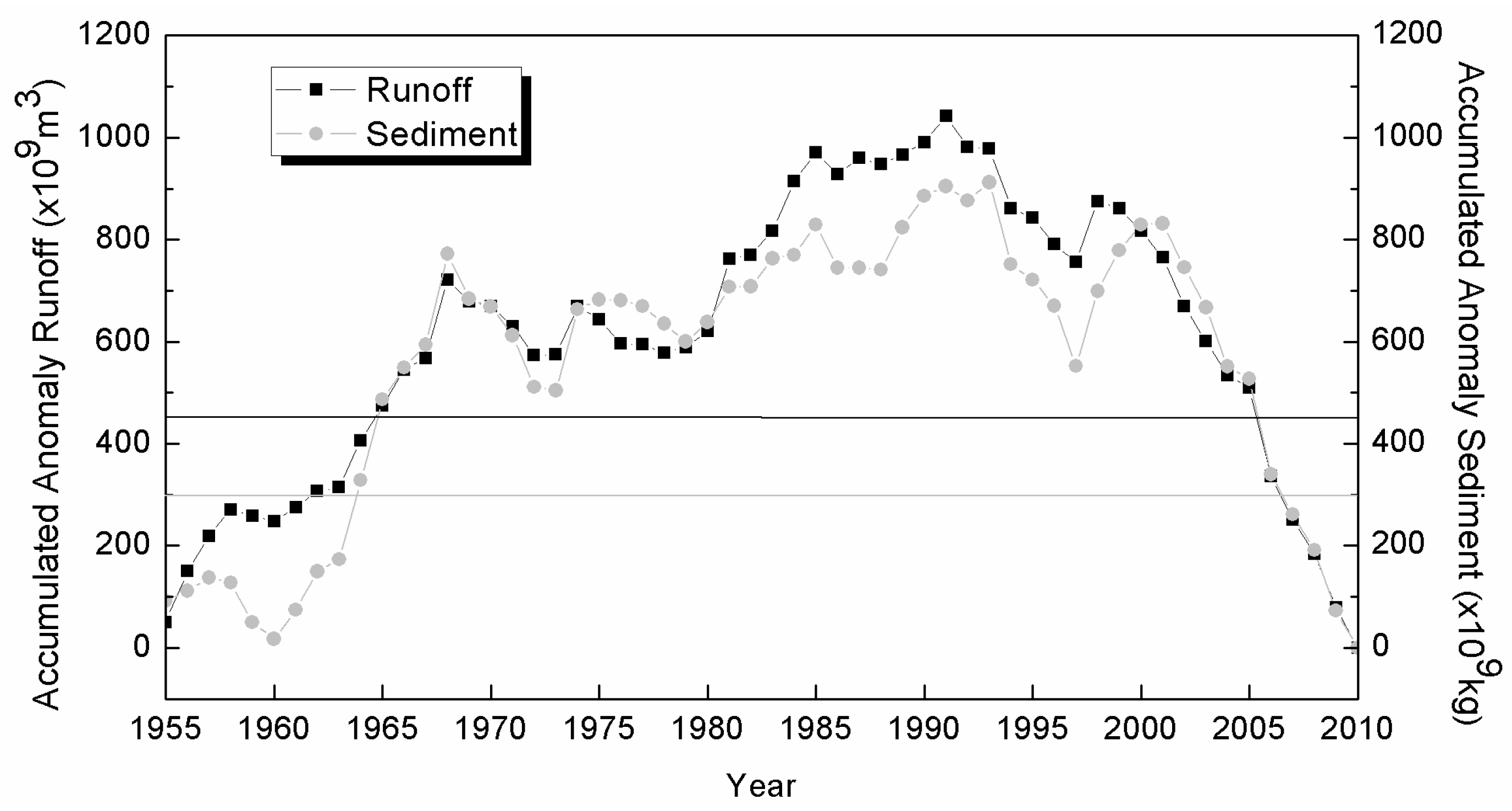
In the demonstration and preliminary design stage, historical hydrological data at Cuntan and Wulong station from 1961 to 1970 were used as the incoming runoff and sediment for the TGP, with a mean annual runoff and sediment of 420 × 109 m3 and 509 × 109 kg, respectively. The Cuntan station lies on the mainstream of the Yangtze River, about 7.5 km away from the confluence of the Jialingjiang River and the Yangtze River, 597 km away from the Three Gorges Dam. The catchment area of the Cuntan station is 8.67 × 10⁵ km2. The Wulong station is on the Wujiang River, which is 71 km away from the estuary with the catchment area of 8.30 × 10⁴ km2. The sum of the data at Cuntan station and Wulong station is regarded as the incoming runoff and sediment into the TGP. After 28 September 2008, the terminal of the backwater of the TGP stretched upstream, and the runoff and sediment characteristics of Cuntan station were obviously affected by the impoundment. Hence, Zhutuo station on the mainstream of the Yangtze River, which is 757 km away from the Three Gorges Dam, Beibei station on the Jialingjiang River, which is 53 km way from the estuary, and the Wulong station are taken as the control stations for the incoming runoff and sediment into the TGP. According to the computational rules above, the statistical annual runoff and sediment into the TGP during the year 1955 to 2010 is shown in Figure 2.
As shown in Figure 2, the inter-annual variation of runoff and sediment in the upper Yangtze River is great. Affected by rainfall conditions as well as underlying surface conditions, the process displays randomness with alternating high and low values, while the sediment transport process is highly synchronized with runoff. The solid line and dotted line in Figure 2 indicate the tendency changes of runoff and sediment in to the TGP, respectively, both of which decrease almost at the same slope. The sediment into the TGP keeps decreasing significantly after 1974, except for the year 1998, when the famous super flood happened in many drainage basins in China. Especially in the last 20 years, both runoff and sediment decreased obviously.
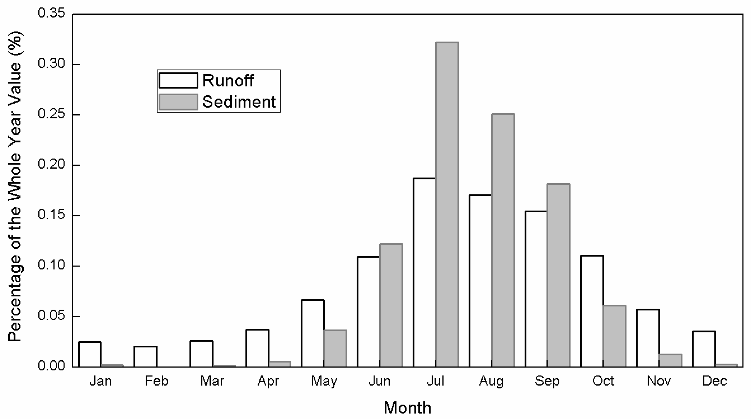
Flood season in the upper Yangtze River is remarkable, resulting in non-uniformity of the runoff and sediment distribution within a year. The percentage of the total yearly runoff and sediment occurring in each month is shown in Figure 3. Both the runoff and sediment are mainly concentrated in flood season, from May to October, when about 80% of the whole year’s runoff and 90% of the whole year’s sediment are yielded. Because rainstorms have a closer relationship with sediment yield than with runoff, the imbalance of sediment is more prominent than that of runoff. About 90% of the annual sediment comes from flood season, and over half of the annual sediment is concentrated in the major flood period of August and September. Most of the sediment is based on several rainstorms and floods.
3. Analysis on Runoff and Sediment Characteristics
The upper reaches of the Yangtze River have a large drainage area with complicated runoff and sediment yield conditions. The runoff process performs cyclical variations with a rising or declining trend, as well as abrupt points resulting from climate change and human activities, such as impounding reservoirs and water usage. For the sediment, because of the complex geological and geomorphological conditions of the upper Yangtze River, as well as the large scale of the area, yield and transport are complicated. Hence, this study only relies on the statistics of the long sequence of historical data, without cause analysis, including trend analysis, abrupt changes analysis, and cyclical analysis.
3.1. Trend Analysis
The trend analysis methods adopted in this study are accumulated anomaly analysis and the Mann-Kendall rank correlation test. Accumulated anomaly analysis [20] is first used to estimate the general trend of runoff and sediment into the TGP, and then the Mann-Kendall rank correlation test is applied to verify the specific tendency. Accumulated anomaly analysis is a frequently-used approach for judging variation trends, and it can also be used to divide the phases of the variation. For a time sequence xi, the accumulated anomaly at moment t is:
where . With the values of St at N moments, the accumulated anomaly curve can be drawn to analyze the tendency.
Among various trend analysis methods, the Mann-Kendall rank correlation test is the most popular, due to its lower requirements on data volume, and the smaller impact on results when data deviate from normality. The ultimate principle of the Mann-Kendall rank correlation test is that: for time series , their dual price P is firstly obtained; i.e., for all , the numbers of is P. If holds for all the values in this time series, then there is an uptrend, and , while if , there is a downtrend and . Therefore, for a sequence without any trend, . If , a downtrend might exist, and if there might be an uptrend. The statistic of U is adopted in this test:
where ; . converges fast to a standardized normal distribution when N increases. Confidence level is set as , critical value is obtained from normal distribution table [21].
By statistical analysis of the runoff of the years 1955 to 2010 into the TGP, the maximum and minimum values are 603.9 × 10⁹ m3 and 276.7 × 10⁹ m3, respectively, and the ratio is thus 2.18. These values of the sediment load are 477.4 × 10⁹ kg and 112.4 × 10⁹ kg, and the ratio between them is 4.25. These results illustrate that there is substantial year-to-year variability in the runoff and sediment, while the variation for sediment is greater than that for runoff. The accumulated anomaly curves of the runoff and sediment into the TGP are shown in Figure 4.
The average annual runoff and sediment from 1955 to 2010 are 450 × 109 m3 and 299 × 109 kg, respectively. Figure 4 shows an incremental trend of the runoff before the year 1991, which reduces significantly after then, especially over the last 10 years. There are also some fluctuations over the entire procedure with inflection points, such as the years 1968, 1974, 1980 and 1985. The latest inflection point appears in 1998, when the well-known flood occurred. The tendency of the sediment load procedure is basically the same as runoff, although sometimes with a ‘time lag’, such as with the crests appearing in 2001. The sediment trend is also more obvious than runoff with larger slope.
According to the results of the Mann-Kendall rank correlation test with N = 55 and confidence level , the annual runoff statistic of runoff , the absolute value of which is larger than , presenting a prominent reduce trend. Meanwhile, for sediment at the Cuntan station , the absolute value of which is also larger than ; thus, the decreasing trend passes the significant test at 0.01 level.
3.2. Abrupt Change Analysis
Abrupt change refers to a change at a certain moment in a time series, with a steep increase or steep drop in the values before and after the jump points. The accumulated anomaly analysis above can be used for observing jump points. Additionally, Fisher’s ordered clustering method is adopted for abrupt change analysis in this study.
Fisher’s ordered clustering method divides an N-sample sequence {xi} into k classes, and searches for an optimal clustering scheme to minimize the sum of the dispersion [22]. There are two features of this method: one is that these N samples are ordered, and the other characteristic is that the continuity of the sample order should be maintained during the clustering without any jump. When splitting the sample sequence, the data within a certain class are supposed to be close. Variance of the class is used to represent the deviation of the data in this segment. The optimal clustering criterion is to achieve minimum variance within a class, and maximum variance among different classes.
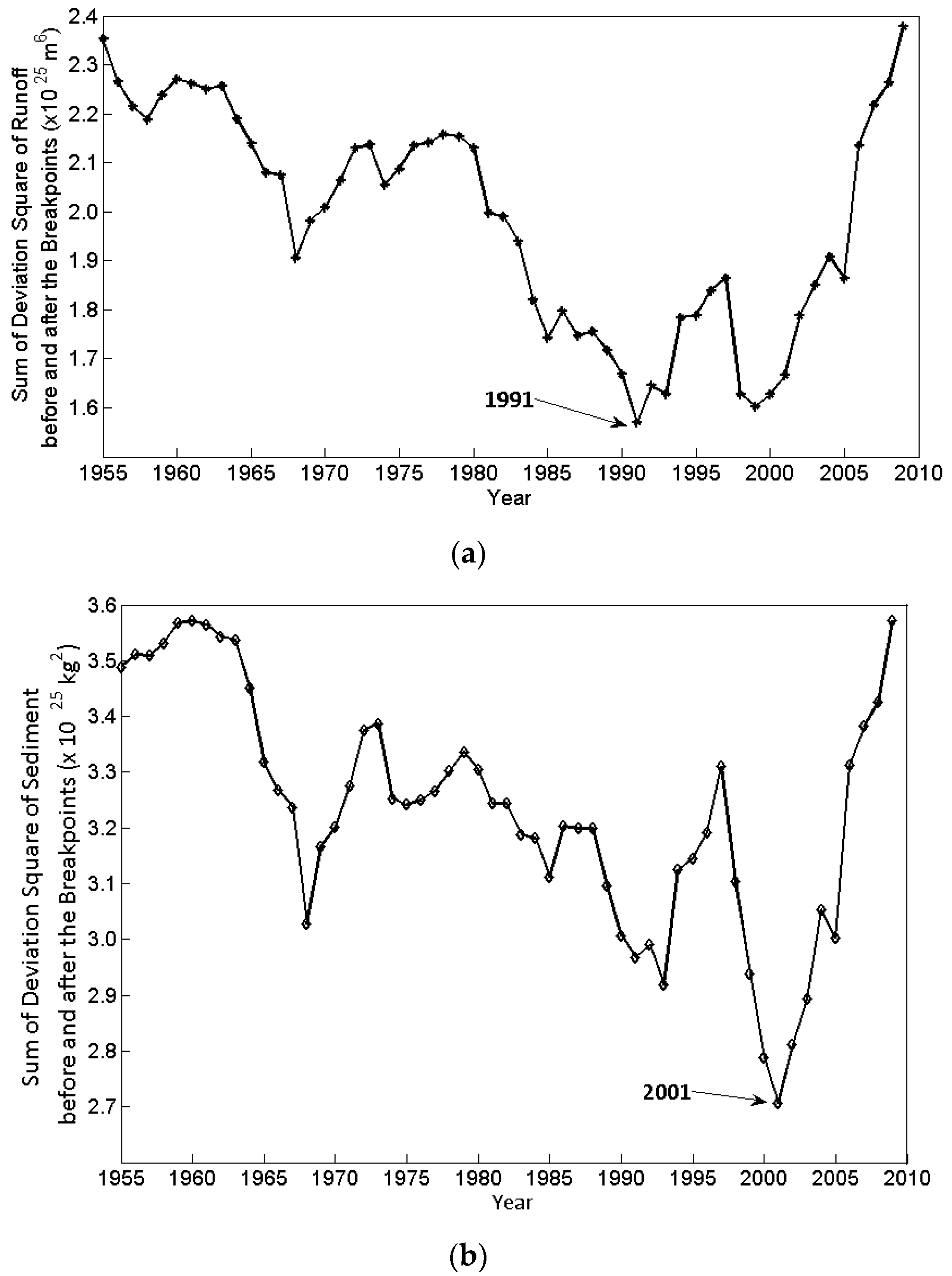
Figure 5 shows the segment result by Fisher’s ordered clustering method of 55 runoff and sediment sequence over the year 1955 to 2010, which implies the years 1991 and 2001 should be the optimal jump points for runoff and sediment clustering, respectively. The classification result by Fisher’s ordered clustering method agrees with the accumulated anomaly curves in Figure 4. Both of the analyses indicate that the years 1991 and 2001 can be taken as jump points where the characteristics of runoff and sediment changed sharply. Taking the segment result as the standard of classification, the average runoff of the two periods before and after 1994 is presented in Table 1, as well as the average sediment of the two periods before and after 2001.
From Table 1, a distinct jump in the runoff into the TGP after the year 1991 can be quantized, the degree of which is −83.02 × 10⁹ m3, −36.81% of the average value of the entire data. The corresponding sediment reduction is 36.81%, with a value of 110.14 × 10⁹ kg.
Such an obvious drop in the incoming runoff and sediment in recent years not only relates to global climate change, but also has a strong relationship with the massive construction of reservoirs upstream. As a result, the reservoir sedimentation problem of the TGR is not as severe as expected when designing and planning. However, the release of clean water may lead to other ecological and environmental issues downstream. For example, various nutrients adhering to sediment particles are essential to aquatic organisms downstream, which will decrease with the drop in sediment. The relationship between the mainstream of the Yangtze River and the lakes along the river may also change when the river bed downstream is lowered by clean water scouring, so that less water can re-enter the lake, resulting in the lake shrinking.
3.3. Cyclical Analysis
Maximum Entropy Spectral Analysis (MESA), which is a parametric modern spectrum analysis method, was introduced by [23]. MESA is based on choosing the spectrum that corresponds to the most random or the most unpredictable time series whose autocorrelation function agrees with the known values. Spectral analysis methods the regard time sequence as a superposition of various regular waves with different frequencies. The main cycle can be determined by comparing the variance of different waves. The maximum entropy spectrum analysis adopts an extrapolation principle as follows: the unknown values have the greatest uncertainty.
The entropy of a stationary sequence is defined as:
where is the spectrum density of the sequence, .
To maximize entropy H, the entropy spectrum has to be in the form as follows, proved by auto-regression model and Lagrangian multiplier:
where f is the frequency, f = 1/T, and T is the cycle. Plot the If of waves with different frequency, if there is a peak in the plot, the corresponding cycle is the prominent cycle. MESA is suitable for a process with unknown basic distribution. The disadvantages of classical spectral analysis, such as subjective assumption of missing data, are overcome by MESA. Especially for short sequences, the major cycle obtained by MESA is of high accuracy.
Figure 6 shows the maximum spectral density estimates results of runoff and sediment into the TGP. The order of the spectrum analysis is set to 50, since the sequence data used in this study is only 55 years. Both the runoff and sediment present a periodical change about every 10 years. The most noticeable cycles for runoff and sediment are 11.4 years and 8.6 years, respectively. These cyclic analysis results are helpful for flood forecasting. On one hand, the flood control can be better prepared by using the reservoirs upstream; on the other hand, the cycle rule can be utilized to flush more sediment downstream when a flood is expected.
4. Prediction Model
Previous analysis shows that both runoff and sediment inflow into the TGP have undergone tendency changes over recent 10 years due to dramatic changes in the environment. Additionally, runoff and sediment are influenced greatly by the seasons. In order to improve prediction accuracy, the historical monthly average data after the TGP was put into operation in January 2003 are adopted to build the forecast model of the runoff and sediment inflow.
4.1. Stationary Processing of the Original Data
In this study, the monthly average runoff and sediment inflow into the TGP from the years 2003 to 2010 are taken as a univariate time series with seasonal variation, and the mixed seasonal and non-seasonal ARIMA model (p, d, q) × (P, D, Q)s is used to build the prediction model.
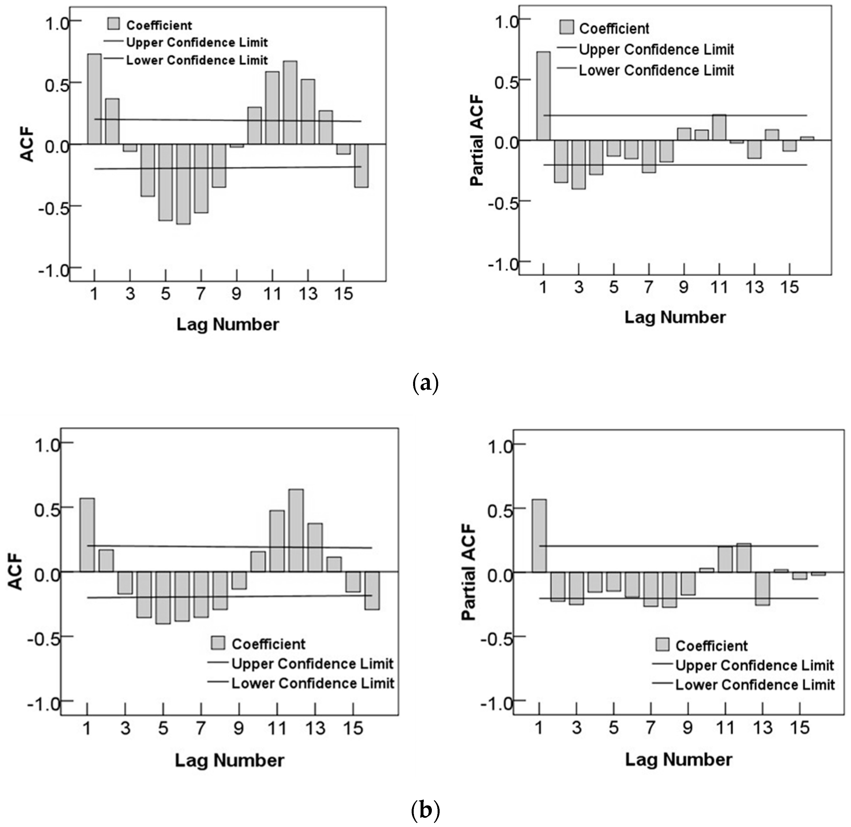
The fundamental assumption for applying the ARIMA model is that the data is stationary, i.e., the sequence has no tendency, nor periodicity. However, both the runoff and sediment load fluctuate with an obvious annual periodicity, with large differences from year to year. It is preliminarily determined that the sequences of runoff and sediment are non-stationary series. To further determine the stationarity, the autocorrelation figures (ACF) and partial autocorrelation figures (Partial ACF) of runoff and sediment are presented in Figure 7.
Stationary sequences typically have short-term correlation, so the coefficient of autocorrelation quickly decays to zero with the increase of the lag number. Conversely, the autocorrelation coefficient of non-stationary sequence decays to zero relatively slowly. As can be seen from Figure 7, the decay speed of ACF is slow, and a lot of the autocorrelation coefficients and partial correlation coefficients fall outside 2 standard deviations. In addition, the autocorrelation figures present a significant sine (cosine) wave, which is a typical feature of a periodic variation of non-stationary sequences. The characteristics of the ACF and Partial ACF figures above imply that the sequences of runoff and sediment have correlations, rather than pure randomness. A stationary processing for the data is required.
Theoretically, the determinate information in a non-stationary sequence can be extracted by differential processing. But such processing causes missing data and lost information. To avoid excessive differentials in practice, differential processing begins at a low order to get the appropriate differential order for smoothing the data. Since the runoff and sediment sequences show notable inter-annual variability, first order differential processing with a step of 12 [24] is carried for the monthly average data. The residual process is shown in Figure 8, which does not appear stationary. To provide the judging criteria, stationary tests—namely ADF unit root tests—are taken. For the ADF test, the returned values are t-Statistics of Augmented Dickey-Fuller test statistics and Test critical values. If the statistical value is smaller than the critical value, it means that at such levels of significance, the null hypothesis of the original sequence having a unit root is refused, and the original series is stationary. The ADF test result for the residuals of runoff and sediment is presented in Table 2.
For the runoff sequence in Table 2, Augmented Dickey-Fuller test statistic = −0.304642 (p = 0.5731), which is larger than the critical values at 1%, 5%, and 10% level. Hence, the null hypothesis that the original sequence has a unit root is accepted, i.e., after removing the seasonal effect, the runoff sequence is not stationary. In the same way, the residuals of sediment sequence without seasonal effect are also not stationary under all the three significant levels. To eliminate the tendency of the data, another first order differential is taken, and the ADF test result is shown in Table 3, which illustrates that both the runoff and the sediment sequences become stationary after removing the seasonal effect and the tendency.
4.2. ARIMA Model
Box and Jenkins [25] proposed a set of methods for analysis, predictions and control of time series, called the Box-Jenkins modeling method. The auto-regressive moving average (ARMA) model is one of the important basic models. Rainfall and sediment yield are usually affected by multiple factors, which are so complex that the traditional regression analysis methods can hardly describe them precisely. The ARMA model uses time elements to take the place of all the other factors with a high degree of accuracy. In addition, ARMA can be used to model sequences with seasonal effects. The time series of rainfall and sediment yield have an apparent seasonal effect, accompanied by long-term trends and random fluctuations. To express the complex relationships among these three factors, the ARMA model with seasonal effect is associated with a short-term correlation model. The ARIMA model is actually a combination of the difference operator and the ARMA model. The mixed effect of the seasonal ARIMA and non-seasonal ARIMA manifests itself in the form of formula (5).
where B is the backward shift operator: , m is the time span; is the backward difference operator: , and d is the difference order; is the auto regressive operator, p is the regressive order, are the parameters of the auto regressive part. are the seasonal auto regressive operators, P is the seasonal regressive order, are the parameters of the seasonal auto regressive part; are the moving average operators, q is the moving average order, are the parameters of the moving average part; are the seasonal moving average operators, Q is the seasonal moving average order, are the parameters of seasonal moving average parts; S is the seasonal cycle.
From the differential processing above, it is easily known that for the ARIMA model ((p, d, q) × (P, D, Q)s), d = 1, s = 12. While for the ARIMA (p, 1, q) × (P, 1, Q)s model, Bayesian information criteria are adopted to determine the order p and q [26]. In this study, the ARIMA (p, 1, q) × (P, 1, Q)s model is tested from low order to find the model with the minimum BIC, which stands for the best goodness-of-fit. Prediction with the determinate model is compared with historical data. The BIC information was minimized in the models ARIMA (1, 1, 1) × (1, 1, 1)12 and ARIMA (0, 1, 1) × (0, 1, 1)12. The comparison of these two models applied to runoff and sediment sequence analysis is shown in Table 4, which implies that the seasonal model ARIMA (1, 1, 1) × (1, 1, 1)12 is the optimal model to present the runoff sequence, while for the sediment sequence, the seasonal model ARIMA (1, 1, 1) × (1, 1, 1)12 is more appropriate with higher accuracy.
Thus, model ARIMA (1, 1, 1) × (1, 1, 1)12 and ARIMA (0, 1, 1) × (0, 1, 1)12 are selected to represent the runoff and sediment sequence into the TGP, respectively, the parameters of which are shown in Table 5.
4.3. Predictions
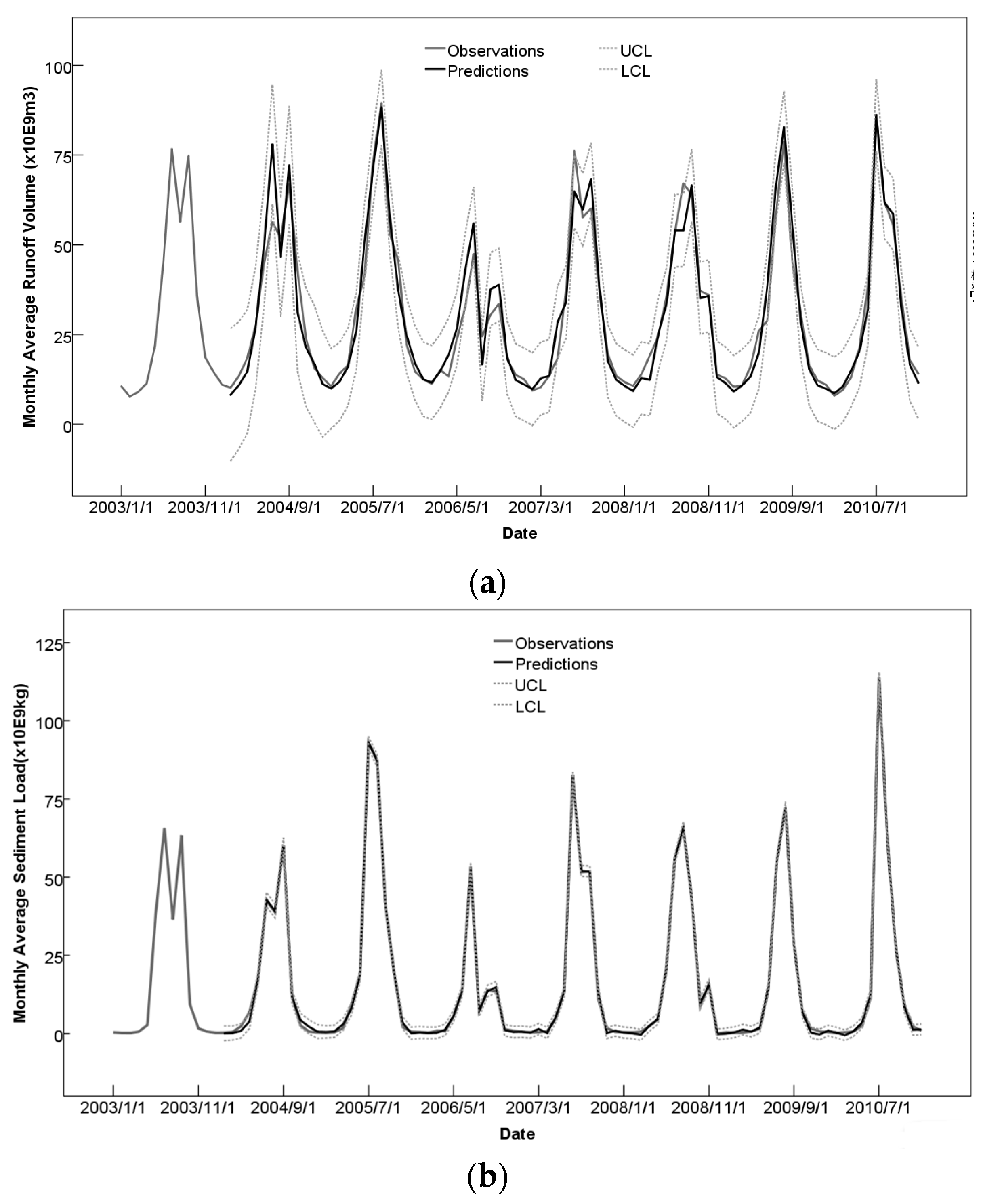
The models ARIMA (1, 1, 1) × (1, 1, 1)12 and ARIMA (0, 1, 1) × (0, 1, 1)12, with parameters as shown in Table 5, are used to predict the runoff and sediment into the TGP, respectively. The results are compared with the historical data, as shown in Figure 9.
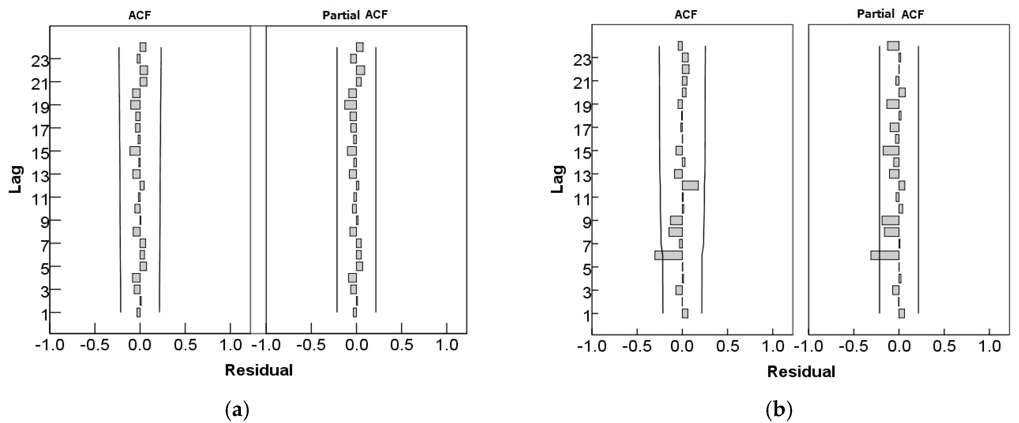
Figure 10 shows the ACF and Partial ACF analysis of the residuals of the model ARIMA (1, 1, 1) × (1, 1, 1)12 for runoff and the residuals of the model ARIMA (0, 1, 1) × (0, 1, 1)12 for sediment sequences. All the autocorrelation coefficients and partial autocorrelation coefficients are within the confidence limits, and the residuals are distributed randomly. Hence, the models above are rational for representing and predicting the runoff and sediment inflow into the TGP with a high level of accuracy.
5. Conclusions
The upper reaches of the Yangtze River play a significant role for the development of downstream areas. As the largest hydropower structure in the world, the Three Gorges Project has aroused public concern since its demonstration. Plenty of previous research focuses on the sediment problems of the reservoir. However, with economic development, the environment has changed a lot, especially in recent decades. This paper takes the hydrological series from the years 1955 to 2010 to analyze the runoff and sediment characteristics into the TGP, and provides results of the variation tendency, the abrupt changes, and the periodicity of the fluctuation. The results indicate that there is a decreasing tendency for both runoff and sediment into the TGP, and jump points of the changes of runoff and sediment appear in the years 1991 and 2001, respectively. Although such a drop in incoming sediment is conducive to reservoir sedimentation, it may lead to new ecological and environmental problems downstream, as the sediment released from the reservoir decreases greatly. The cycles of the fluctuation are also presented, which are around 10 years. Using the monthly average data from 2003 to 2010, ARIMA models are built to predict the runoff and sediment into the TGP. Seasonal mixed model ARIMA (1, 1, 1) × (1, 1, 1)12 and ARIMA (0, 1, 1) × (0, 1, 1)12 are finally selected to represent the runoff and sediment sequence into the TGP, and the parameters are also calibrated. Autocorrelation and partial autocorrelation analysis illustrates that the models can be used to represent the runoff and sediment into the TGP with a high level of accuracy. The accurate forecast of incoming runoff and sediment not only helps for the flood control, but can also be made use of for flushing more sediment downstream when the flood comes, so as to alleviate the ecological and environmental problems resulting from the sediment reduction.
Acknowledgments
This research was supported by the National Key Research and Development Program of China (Grant No. 2016YFC0402405, 2016YFC0401301), the Open Research Fund of the State Key Laboratory of the Changjiang River Scientific Research Institute of the Changjiang Water Resources Commission (Grant No. CKWV2015204/KY), and the National Natural Science Foundation of China (Grant No. 51409248).
Author Contributions
Jun Qiu and Fang-Fang Li conceived and designed the experiments; Chun-Feng Hao performed the experiments; Chun-Feng Hao and Jun Qiu analyzed the data; Fang-Fang Li contributed reagents/materials/analysis tools; Fang-Fang Li wrote the paper.
Conflicts of Interest
The authors declare no conflict of interest.
References
- Sivakumar, B.; Berndtsson, R.; Persson, M. Monthly runoff prediction using phase space reconstruction. Hydrol. Sci. J. 2001, 46, 377–387. [Google Scholar] [CrossRef]
- Smith, J.A. Long-range streamflow forecasting using non-parametric regression. Water Resour. Bull. 1991, 27, 39–46. [Google Scholar] [CrossRef]
- Irvine, K.N.; Eberhardt, A.J. Multiplicative, season ARIMA models for Lake Erie and Lake Ontario water levels. Water Resour. Bull. 1992, 28, 385–396. [Google Scholar] [CrossRef]
- Uvo, C.B.; Graham, N.E. Seasonal runoff forecast for northern Southern America: A statistical model. Water Resour. Res. 1998, 34, 3515–3524. [Google Scholar] [CrossRef]
- Chiew, F.H.S.; Zhou, S.L.; McMahon, T.A. Use of seasonal streamflow forecasts in water resources management. J. Hydrol. 2003, 270, 135–144. [Google Scholar] [CrossRef]
- Shentzis, I.D. Mathematical models for long-term prediction of mountainous river runoff methods, information and results. Hydrol. Sci. J. 1990, 35, 487–500. [Google Scholar] [CrossRef]
- Druce, D.J. Insights from a history of seasonal inflow forecasting with a conceptual hydrological model. J. Hydrol. 2001, 249, 102–112. [Google Scholar] [CrossRef]
- White, S. Sediment yield prediction and modeling. In Encyclopedia of Hydrological Sciences; John Wiley and Sons, Ltd.: New York, NY, USA, 2005. [Google Scholar]
- Singh, V.P.; Krstanovic, P.F.; Lane, L.J. Stochastic models of sediment yield. In Modeling Geomorphological Systems; Anderson, M.G., Ed.; John Wiley and Sons Ltd.: New York, NY, USA, 1998; Volume 2, pp. 272–286. [Google Scholar]
- Yang, C.T. Sediment Transport, Theory and Practice; McGraw-Hill: New York, NY, USA, 1996. [Google Scholar]
- Cohn, T.A.; Caulder, D.L.; Gilroy, E.J.; Zynjuk, L.D.; Summers, R.M. The validity of a simple statistical model for estimating fluvial constituent loads: An empirical study involving nutrient loads entering Chesapeake Bay. Water Resour. Res. 1992, 28, 2353–2363. [Google Scholar] [CrossRef]
- Forman, S.L.; Pierson, J.; Lepper, K. Luminescence geochronology. In Quaternary Geochronology: Methods and Applications; Sowers, J.M., Noller, J.S., Lettis, W.R., Eds.; American Geophysical Union Reference Shelf: Washington, DC, USA, 2000; Volume 4, pp. 157–176. [Google Scholar]
- Partal, T.; Cigizoglu, H.K. Estimation and forecasting of daily suspended sediment data using wavelet-neural networks. J. Hydrol. 2008, 358, 317–331. [Google Scholar] [CrossRef]
- Sivakumar, B. Suspended sediment load estimation and the problem of inadequate data sampling: A fractal view. Earth Surf. Process. Landf. 2006, 31, 414–427. [Google Scholar] [CrossRef]
- Yu, W.C.; Yue, H.Y. Position of runoff and sediment of Yangtze River in world rivers. J. Yangtze River Sci. Res. Inst. 2002, 19, 13–16. (In Chinese) [Google Scholar]
- ChangJiang Water Resources Commission of the Ministry of Water Resources (CJW). 2011 Sediment Communique of the Yangtze River; Yangtze River Press: Wuhan, China, 2012; p. 5. (In Chinese) [Google Scholar]
- Schumm, S.A. The Fluvial System; John Wiley and Sons Ltd.: New York, NY, USA, 1977; 338p. [Google Scholar]
- Guo, S.L.; Xu, G.H.; Zhang, X.T.; Bian, W. Influence of ‘soil erosion control project’ on incoming sediment of Three Gorges Reservoir. Yangtze River 2004, 35, 1–6. (In Chinese) [Google Scholar]
- Liu, Y. Effect of key upstream sediment-producing zones on water flow and sediment charge into the Three Gorges Reservoir. China Three Gorges Constr. 1995, 5, 24–25. (In Chinese) [Google Scholar]
- Wei, F.Y. Diagnostic Statistical Prediction of Modern Climate; China Meteorological Press: Beijing, China, 2007. (In Chinese) [Google Scholar]
- Kendall, M.G.; Gibbons, J.D. Rank Correlation Methods, 5th ed.; Oxford University Press: New York, NY, USA, 1990. [Google Scholar]
- Fisher, D.H. Knowledge acquisition via incremental conceptual clustering. Mach. Learn. 1987, 2, 139–172. [Google Scholar] [CrossRef]
- Burg, J.P. Maximum entropy spectral analysis. Presented at 37th Annual International Meeting, Society of Exploration Geophysicists, Oklahoma City, OK, USA, 31 October 1967. [Google Scholar]
- Zhang, X.J.; Zhang, X.L. Application of time series analysis model on total corn yield of Shandong province. Res. Soil Water Conserv. 2007, 14, 3–5. (In Chinese) [Google Scholar]
- Box, G.P.E.; Jenkis, G.M. Time Series Analysis: Forecasting and Control, 2nd ed.; San Francisco Press: San Francisco, CA, USA, 1976. [Google Scholar]
- Wang, Y. Applied Time Series Analysis; China Renmin University Press: Beijing, China, 2005. (In Chinese) [Google Scholar]
Figure 1.
River system diagram of the upper reaches of the Yangtze River.
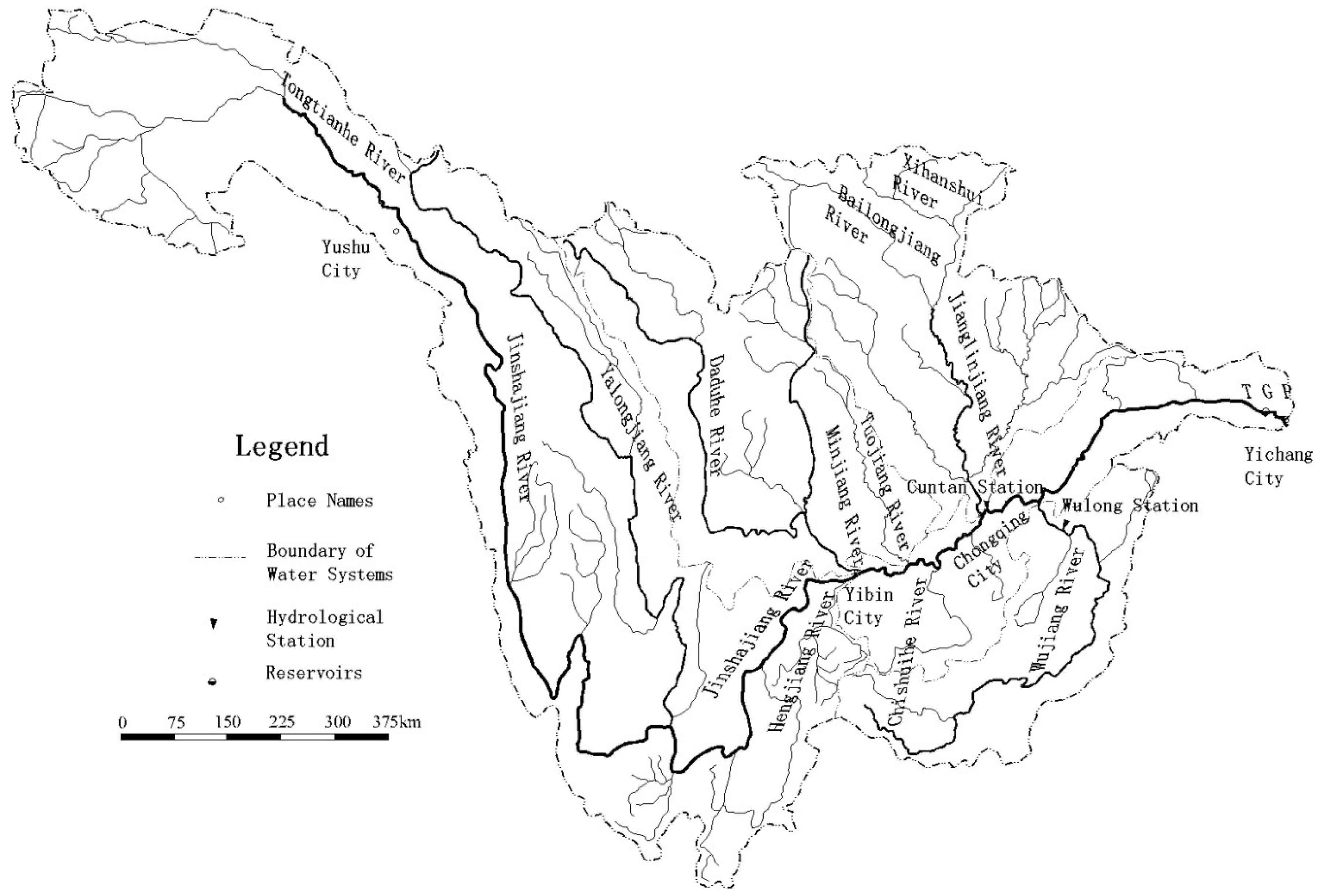
Figure 2.
Annual runoff and sediment into the TGP.
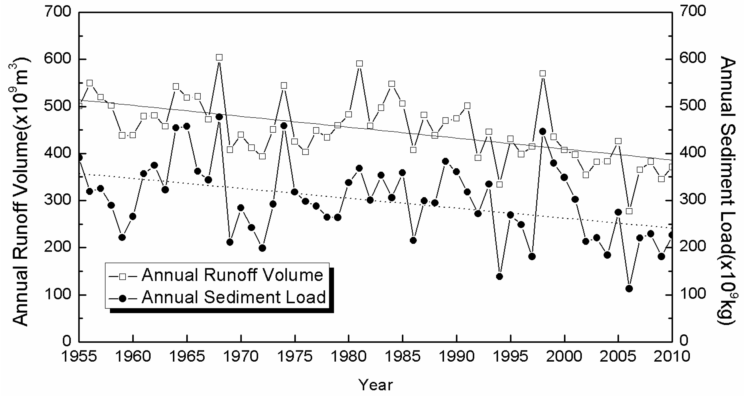
Figure 3.
Monthly percentages of runoff and sediment load.

Figure 4.
Accumulated Anomaly Curves of Runoff and Sediment during 1955 to 2010.

Figure 5.
Fisher’s ordered clustering curves of runoff and sediment into the TGP: (a) Runoff; (b) Sediment.
Figure 5.
Fisher’s ordered clustering curves of runoff and sediment into the TGP: (a) Runoff; (b) Sediment.

Figure 6.
Maximum spectral density estimates of runoff and sediment into the TGP: (a) Runoff; (b) Sediment.
Figure 6.
Maximum spectral density estimates of runoff and sediment into the TGP: (a) Runoff; (b) Sediment.
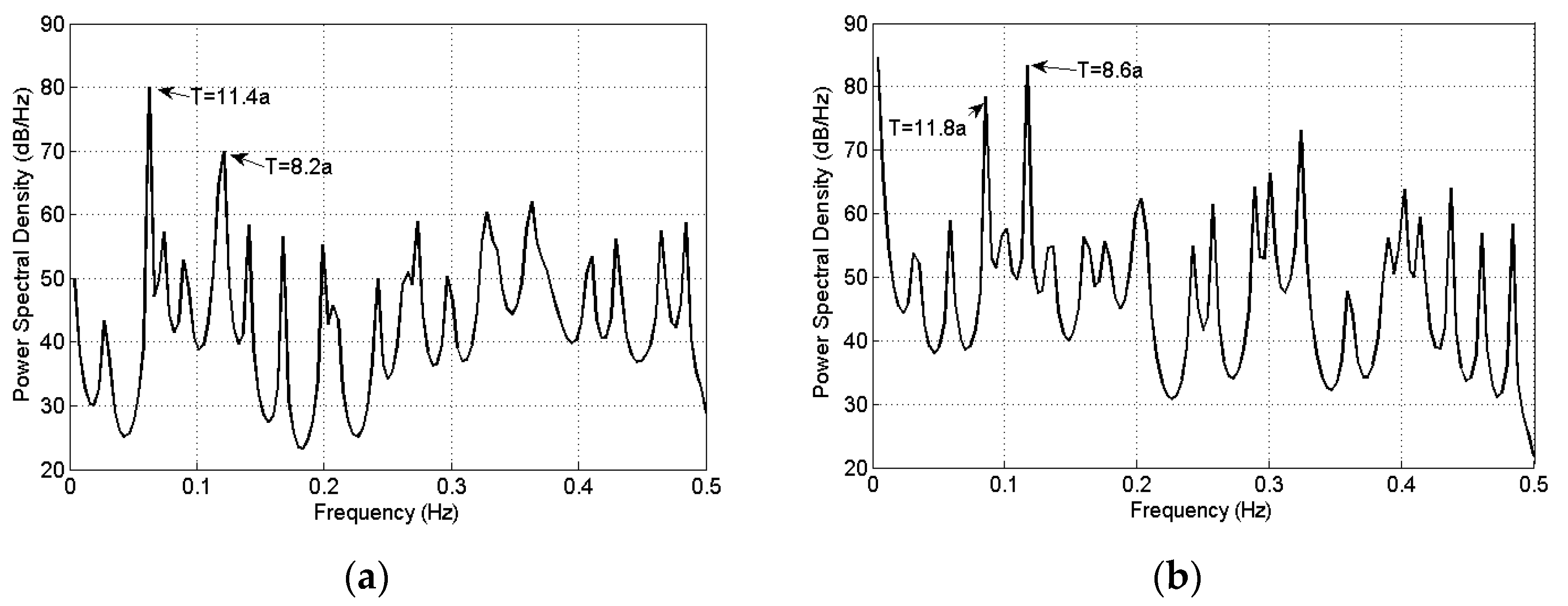
Figure 7.
ACF and PACF of Runoff and Sediment into the TGP: (a) Runoff; (b) Sediment.

Figure 8.
Sequences after removing seasonal effect.
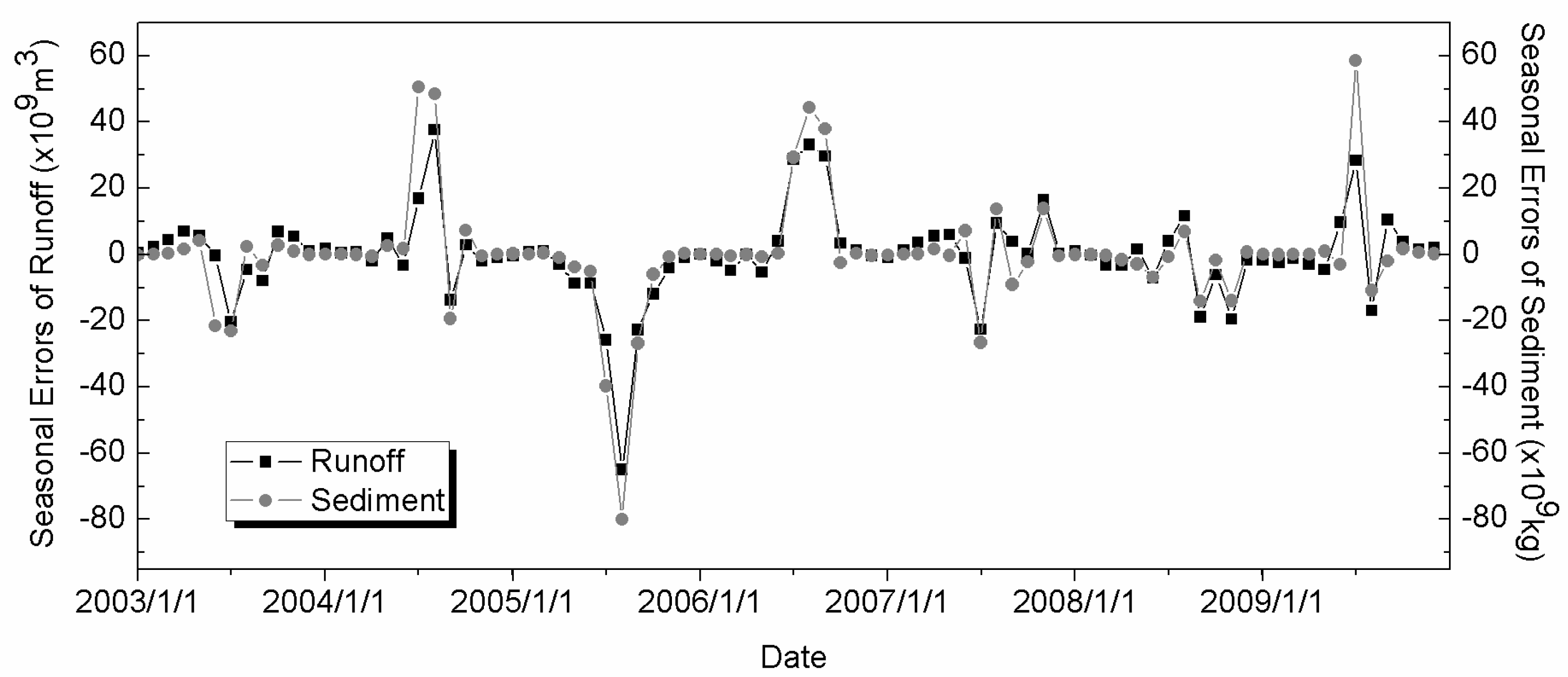
Figure 9.
Predictions by ARIMA model: (a) Runoff; (b) Sediment.

Figure 10.
ACF and Partial ACF of ARIMA model: (a) Runoff; (b) Sediment.

Table 1.
Annual average value of runoff and sediment inflow of reservoir TGP before and after abrupt.
Table 1.
Annual average value of runoff and sediment inflow of reservoir TGP before and after abrupt.
| Period | 1955–1991 | 1992–2010 | Difference |
| Runoff a (×109 m3) | 478.19 | 395.17 | −83.02 (−18.45%) |
| Period | 1955–2001 | 2002–2010 | Difference |
| Sediment b (×109 kg) | 316.91 | 206.77 | −110.14 (−36.81%) |
Table 2.
ADF test results of residuals removing the seasonal effect a.
| Runoff | Sediment | ||||
|---|---|---|---|---|---|
| t-Statistic | Prob. b | t-Statistic | Prob. b | ||
| Augmented Dickey-Fuller test statistic | −0.304642 | 0.5731 | −0.497882 | 0.4977 | |
| Test critical values | 1% level | −2.593121 | −2.593121 | ||
| 5% level | −1.944762 | −1.944762 | |||
| 10% level | −1.614204 | −1.614204 | |||
Notes: a Null Hypothesis: SEQUENCE has a unit root; Exogenous: None; Lag Length: 12 (Fixed); b MacKinnon (1996) one-sided p-values.
Table 3.
ADF test results of residuals removing the seasonal effect and the tendency a.
| Runoff | Sediment | ||||
|---|---|---|---|---|---|
| t-Statistic | Prob. b | t-Statistic | Prob. b | ||
| Augmented Dickey-Fuller test statistic | −4.681944 | 0.0000 | −4.661704 | 0.0000 | |
| Test critical values: | 1% level | −2.593468 | −2.593468 | ||
| 5% level | −1.944811 | −1.944811 | |||
| 10% level | −1.614175 | −1.614175 | |||
Notes: a Null Hypothesis: SEQUENCE has a unit root; Exogenous: None; Lag Length: 12 (Fixed); b MacKinnon (1996) one-sided p-values.
Table 4.
Statistics of ARIMA model fitting for runoff and sediment sequences.
| ARIMA Model | Statistics of Model Fitting | ||||||||
|---|---|---|---|---|---|---|---|---|---|
| Stationary R2 | R2 | RMSE | MAPE | MAE | MaxAPE | MaxAE | BIC of Normal | ||
| Runoff | (0, 1, 1) × (0, 1, 1)12 | 0.779 | 0.892 | 71.577 | 14.231 | 43.895 | 47.602 | 235.637 | 8.914 |
| (1, 1, 1) × (1, 1, 1)12 | 0.870 | 0.936 | 56.827 | 12.581 | 36.084 | 54.223 | 216.543 | 8.719 | |
| Sediment | (0, 1, 1) × (0, 1, 1)12 | 0.998 | 0.999 | 9.454 | 52.388 | 5.472 | 918.366 | 30.002 | 5.930 |
| (1, 1, 1) × (1, 1, 1)12 | 0.980 | 0.988 | 31.585 | 52.521 | 19.377 | 228.550 | 84.328 | 7.917 | |
Table 5.
Parameters of ARIMA model.
| Estimation | SE | t | Sig. | |||
|---|---|---|---|---|---|---|
| Runoff | Model | −0.202 | 0.277 | −0.728 | 0.469 | |
| (1, 1, 1) × (1, 1, 1)12 | 0.430 | 0.135 | 3.177 | 0.002 | ||
| 1 | ||||||
| 0.982 | 0.156 | 6.294 | 0.000 | |||
| −0.715 | 0.122 | −5.877 | 0.000 | |||
| 1 | ||||||
| 0.133 | 0.197 | 0.676 | 0.501 | |||
| Sediment | (0, 1 ,1) × (0, 1, 1)12 | −0.081 | 1.072 | −0.075 | 0.940 | |
| 1 | ||||||
| 0.342 | 0.147 | 2.327 | 0.024 | |||
| 1 | ||||||
| −0.989 | 4.672 | −0.212 | 0.833 | |||
© 2017 by the authors. Licensee MDPI, Basel, Switzerland. This article is an open access article distributed under the terms and conditions of the Creative Commons Attribution (CC BY) license (http://creativecommons.org/licenses/by/4.0/).
Share and Cite
MDPI and ACS Style
Hao, C.-F.; Qiu, J.; Li, F.-F. Methodology for Analyzing and Predicting the Runoff and Sediment into a Reservoir. Water 2017, 9, 440. https://doi.org/10.3390/w9060440
AMA Style
Hao C-F, Qiu J, Li F-F. Methodology for Analyzing and Predicting the Runoff and Sediment into a Reservoir. Water. 2017; 9(6):440. https://doi.org/10.3390/w9060440
Chicago/Turabian StyleHao, Chun-Feng, Jun Qiu, and Fang-Fang Li. 2017. "Methodology for Analyzing and Predicting the Runoff and Sediment into a Reservoir" Water 9, no. 6: 440. https://doi.org/10.3390/w9060440
Note that from the first issue of 2016, this journal uses article numbers instead of page numbers. See further details here.