
Modelling of Violent Water Wave Propagation and Impact by Incompressible SPH with First-Order Consistent Kernel Interpolation Scheme

1
College of Shipbuilding Engineering, Harbin Engineering University, Harbin 150001, China
2
School of Mathematics, Computer Science and Engineering, City, University of London, London EC1V 0HB, UK
3
Department of Civil and Structural Engineering, University of Sheffield, Sheffield S1 3JD, UK
4
Department of Civil and Earth Resources Engineering, Kyoto University, Kyoto 615-8540, Japan
*
Author to whom correspondence should be addressed.
Water 2017, 9(6), 400; https://doi.org/10.3390/w9060400
Submission received: 30 April 2017
/
Revised: 27 May 2017
/
Accepted: 31 May 2017
/
Published: 4 June 2017
(This article belongs to the Special Issue Modeling of Water Systems)
Abstract
:The Smoothed Particle Hydrodynamics (SPH) method has proven to have great potential in dealing with the wave–structure interactions since it can deal with the large amplitude and breaking waves and easily captures the free surface. The paper will adopt an incompressible SPH (ISPH) approach to simulate the wave propagation and impact, in which the fluid pressure is solved using a pressure Poisson equation and thus more stable and accurate pressure fields can be obtained. The focus of the study is on comparing three different pressure gradient calculation models in SPH and proposing the most efficient first-order consistent kernel interpolation (C1_KI) numerical scheme for modelling violent wave impact. The improvement of the model is validated by the benchmark dam break flows and laboratory wave propagation and impact experiments.
1. Introduction
The wave propagation and its impact on structure is a common natural phenomenon that is very important in the field of ocean and coastal engineering. During this process, the waves involve with large deformation of free surface, wave breaking, wave run-up and their strong interactions with the structures. Thus, modelling of wave system is of great interest but is also a difficult task in both physical experiments and the numerical simulations.
There are generally two classes of models for wave simulations. In the early years, the Laplace equation with fully nonlinear boundary conditions was used for simple wave problems [1,2,3], while the Navier–Stokes (N-S) equations with more realistic physical boundary conditions were solved in recent numerical models [4,5]. As a result, various numerical schemes, such as the finite element, finite volume and finite difference methods have been used to solve the N-S equations to investigate the nonlinear water wave propagation and its interaction with the structures [6,7]. To relieve the CPU expense and meanwhile provide reasonable solutions for the large domain problems, different forms of the Shallow Water Equations (SWEs) are also proposed in the modelling of wave system [8].
In the last two decades, the Smoothed Particle Hydrodynamics (SPH) method has emerged as a promising mesh-free Lagrangian modelling technique. Although the SPH model may use more CPU time than the grid counterpart in some cases, it has the advantage of tracking the free surface in an easy and accurate way. In this approach, the governing equations are discretized and solved by the individual particles within the computational domain. SPH was originally developed for the study of astrophysics [9,10] and then employed to study the wave propagating and overtopping over coastal structures [11]. Based on the algorithm of the Moving Particle Semi-implicit (MPS) approach [12] and SPH projection method [13], a strict incompressible algorithm of the SPH model [14] was developed and then it was further improved to simulate wave breaking and post-breaking [15]. The major difference between the standard weakly compressible SPH (WCSPH) [9,10] and the incompressible SPH [14] lies in that the former calculates the fluid pressure explicitly by using an equation of state, while the latter employs a strict incompressible formulation to solve the pressure implicitly by a pressure Poisson equation (PPE). Both the WCSPH and ISPH show capabilities and limitations. For WCSPH, it has been highlighted the better possibility to parallelize the numerical code for simulations in real conditions [16]. The pressure field has also been improved by different form of diffusive terms in the continuity equation for wave–structure interaction problems [17,18]. Furthermore, the acoustic components related to the use of the state equation can be eliminated by an appropriate filtering in the data post-processing to recover the incompressible solution [19]. For the impact problems, it has been noticed that ISPH sometimes shows singularities since the pressure is inversely proportional to the adopted time step [20]. On the other hand, the numerical time stepping length of ISPH can be larger than that of WCSPH, so the general computational efficiency could be higher [21,22].
In this paper, an incompressible SPH model will be employed to simulate solitary wave propagation and impact on a slope with different conditions. Although the ISPH model could predict stable and noise-free pressure field in many cases, the numerical accuracy and efficiency could be compromised in the free surface water waves. Among a variety of influence factors, the calculation of pressure gradient plays a very important role in the process. Thus, the current study presents an improved first-order derivative of pressure model for the violent wave simulations, from the first-order consistent kernel interpolation scheme (C1_KI). The proposed C1_KI ISPH model is first verified by the benchmark dam break flow and solitary wave propagation over a constant depth. Then, the wave propagation and impact on an inclined wall are investigated under different slope angles based on the self-designed laboratory experiment.
2. ISPH Methodology
2.1. Governing Equations and Solution Algorithms
The Navier–Stokes (N-S) equations are used to describe the fluid motion. In the incompressible SPH method, the fluid density is considered to be a constant, and therefore the mass and momentum conservation equations are written in the Lagrangian form as follows:
where is the fluid density; is the particle velocity; is the time; is the particle pressure; is the gravitational acceleration; and is the kinematic viscosity. A two-step projection method is used to solve the velocity and pressure field from Equations (1) and (2). The first step is the prediction of velocity in the time domain without considering the pressure term. The intermediate particle velocity and position are obtained by
where and are the velocity and position at time ; is the time step; is the velocity increment; and and are the intermediate velocity and position of particle.
The second step is the correction step in which the pressure term is added, and is the correction of particle velocity
The following and represent the velocity and position of particle at new time step
Combining Equations (1)–(6), the following pressure Poisson equation (PPE) is obtained
Similarly, Shao and Lo [14] proposed a projection-based incompressible approach by imposing the density invariance on each particle, leading to the following PPE:
where is the particle density at intermediate time step. Due to being very close to unity, the difference between the left- and right-hand sides of the denominator in Equation (10) can be ignored, and the combined PPE incorporating both the divergence-free and density-invariance terms is obtained as:
where is a blending coefficient and a value of 0.01 is adopted in this paper from the computational experience. In this paper, only a 2D ISPH formulation is used.
2.2. Calculation of Spatial Derivatives
A common approach to calculate the gradient of pressure and the divergence of velocity is through the following equations:
where is defined; is the gradient of SPH kernel function and a cubic spline kernel [10] is used; is the particle mass; is the kernel smoothing length; is the total neighbouring particle number; and and indicate the reference and neighbouring particles, respectively.
The viscosity term in Equation (2) adopts the following form
where is a small parameter to avoid singularity; and is defined. The Laplacian term in Equation (11) is discretised by combining the SPH gradient and divergence rules to obtain
where is defined.
2.3. Free Surface and Solid Boundary Conditions
The dynamic free surface conditions require a prescribed pressure to be imposed on the surface particles, such as through P = 0. In this paper, we use three auxiliary functions combined with the ratio of particle number density to accurately identify the free surface particles. This has shown to be more robust than using either the density or the divergence rules in conventional ISPH practice. The particles on the solid boundary should satisfy the pressure boundary condition, which is represented by the following momentum balance as
where is the unit vector normal to the solid boundary. More detailed procedures to implement the free surface and solid boundary conditions can be referred to Zheng [21].
3. Improved First-Order Derivative Scheme
In this section three pressure calculation models are compared and an optimum is chosen to use in the practical water wave simulations.
3.1. Simplified Finite Difference Interpolation (SFDI) Scheme
In the traditional SPH calculation of pressure gradient in Equation (12), the computational results are heavily affected by the particle distributions and the shape of solid boundary. To improve this, the first-order derivative of pressure on the solid boundary was formulated by the Simplified Finite Difference Interpolation (SFDI) scheme originally proposed by Sriram and Ma [23] in their MLPG_R approach. SFDI is a second-order accurate scheme based on the Taylor series expansion, which can also be used for the inner fluid particles. In the 2D case, the pressure gradient model formulated by SFDI can be found in [24]. The relevant key formulas are summarized as follows:
where = 1 and = 2 or = 2 and = 1; is the number of neighbouring particles affecting particle ; = and = ; is the component of position vector in (or ) direction.
3.2. Moving Least Square (MLS) Method
MLS is a widely used interpolation scheme for meshless kernel approximation, which can get very high accuracy for the function estimation. Atluri and Shen [25] and Zheng et al. [26] have done many comparisons of improved meshless interpolation schemes with the MLS method. More details of MLS method for the function estimation and first order derivative calculation can refer to Zheng et al. [26]. The accuracy of MLS scheme is very high and the calculation process is more complex than the other traditional meshless interpolation methods. Although the dimension of matrix is not large, the computational cost is demanding as it includes successive multiplication of several matrices and matrix inversions. Although MLS has been widely used for the meshless interpolation comparison [24,26,27], it is less documented in the wave propagation simulations. The key formulations of MLS are summarized as follows.
The unknown function is represented by as
where is the number of nodes that affect the function at ; and is the interpolation or shape function given by
Assume the basis function to be linear
and define the matrix and as
where and are respectively expressed by
and is a weight function which can adopt different forms.
The gradient of the unknown function Equation (20) is estimated by
The partial derivative of shape function with respect to can be directly differentiated as
where is the partial derivative of , i.e., ; and is the -th column of , for which the partial derivative is calculated as
3.3. First-Order Consistent Kernel Interpolation (C1_KI) Scheme
The standard SPH practice widely uses the following symmetric summation form to calculate the first-order derivative as
However, the above equation was based on the assumption of ( is the particle volume), which cannot be exactly satisfied when the particles are disorderly distributed or near the solid boundary. To improve this, the present paper applies the Taylor series expansion of at point , then multiplies this by a kernel function and integrates over its support domain.
Eventually it gives the values of , and in the following matrix form
This method is easy to be expanded to 3D and higher-order problems. As known from Equation (32), when the distributed particles are symmetric about , the error terms become , , and , so all of , and can achieve the second-order accuracy of . On the other hand, when the distributed particles are asymmetric about , the error terms become and , so only can reach the second-order accuracy of , while and merely obtain the first-order accuracy of . Higher-order accuracy results can always be made available by keeping more terms in the Taylor series expansions. More details on the relevant analysis can be found in [26]. The pressure gradient scheme proposed in this section is named as C1_KI, because it can keep the first-order consistency of the gradient estimation. The scheme has the following attractive features. First, it avoids the kernel gradient calculation. The matrix is strictly symmetric, in which only the upper triangle elements need to be calculated and the other elements can be obtained from the symmetric relationships. Besides, it is the first time to combine the C1_KI concept with the truly incompressible SPH scheme, which is expected to inherit the merits of both and therefore provide more accurate violent wave simulations.
4. Convergence and Accuracy of Different Pressure Gradient Models
In this section, several investigations are made into the convergence and accuracy behaviours of the three pressure gradient models, under the uniform and random particle distributions. The error of the numerical results is quantified as
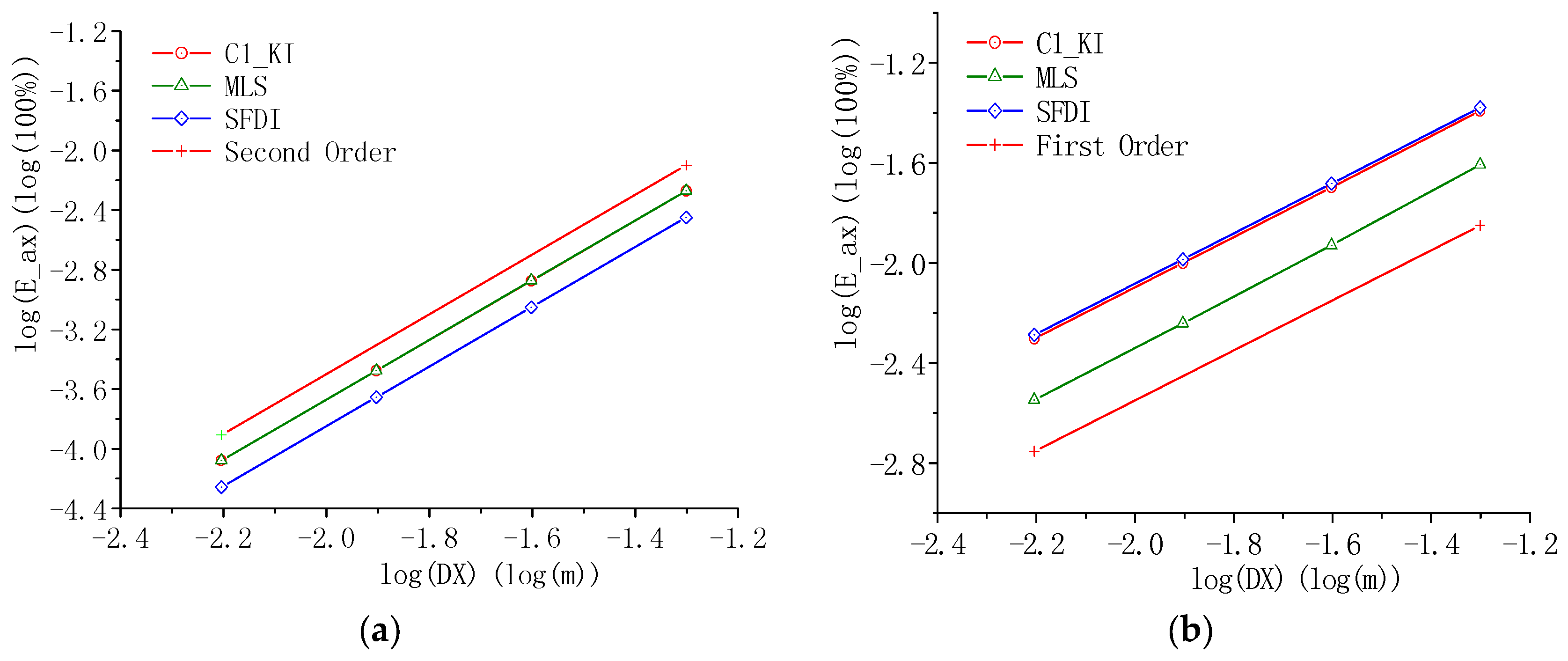
where is the defined mean error; is the numerical value of the gradient component; is the analytical solution; and is the number of sampling points in the inner fluid domain or near the boundary area. Here, the near boundary area is defined as the inner region at a distance of 2 (twice of the particle spacing) from the computational boundary and the remaining area inside is the inner fluid area.
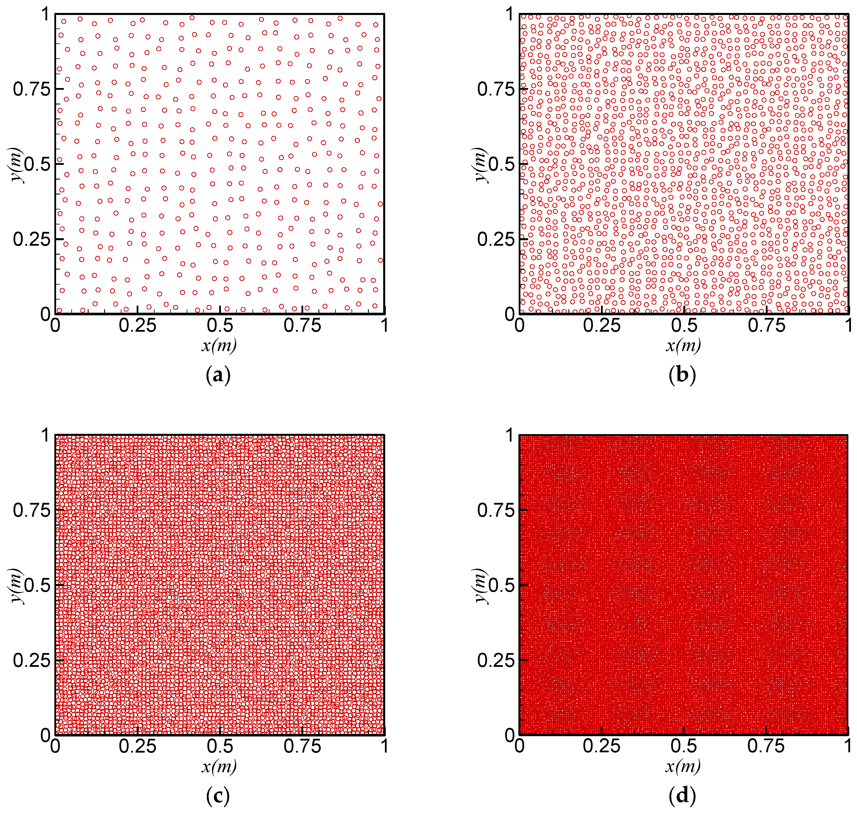
The computational domain of the test is chosen as a square with side length being of 1 m as shown in Figure 1a-d. The test function uses a polynomial function of second order expressed by . The calculation nodes are irregularly distributed in the domain by using the quasi-random number generator. The sample node distributions are illustrated in Figure 1, for the particle number of 400, 1600, 6400 and 25,600, respectively, corresponding to the particle size of 0.05 m, 0.025 m, 0.0125 m and 0.00625 m.
When the particles are uniformly distributed, the convergence rate of the inner domain and near boundary area is shown in Figure 2a,b, respectively. It is shown from Figure 2a that can reach the second-order accuracy for all three pressure gradient methods in the inner fluid domain. Among these SFDI can get the highest accuracy, while the errors of C1_KI and MLS are almost the same. As shown in Figure 2b near the boundary area, MLS can achieve the best results with minimum error while C1_KI performs similarly to SFDI to achieve first-order accuracy. On the other hand, Figure 3a suggests that when the particles are randomly distributed, C1_KI can achieve the most promising results in the inner fluid domain. In the area near the boundary as shown in Figure 3b, both C1_KI and MLS obtain similar results which are better than those computed by SFDI.
Generally speaking, Figure 3 implies that all of the three pressure gradient models can only achieve the first-order accuracy when the particles are irregularly distributed. In practical water wave modelling, the situation of particle randomness should increase from the wave propagation to wave–structure interaction cases because there are frequent exchanges of location within neighbour particles and surface-to-inner particles. Computationally, MLS is the most expensive one since it includes quite a few inverse calculations and matrix multiplications [24,26]. Overall, C1_KI scheme performs quite satisfactory among the three in view of computational accuracy under all tested conditions, thus it will be used to study the wave propagation and impact in the next model applications.
5. Model Applications in Water Wave Modelling
5.1. Dam Break Wave Impact on a Vertical Wall
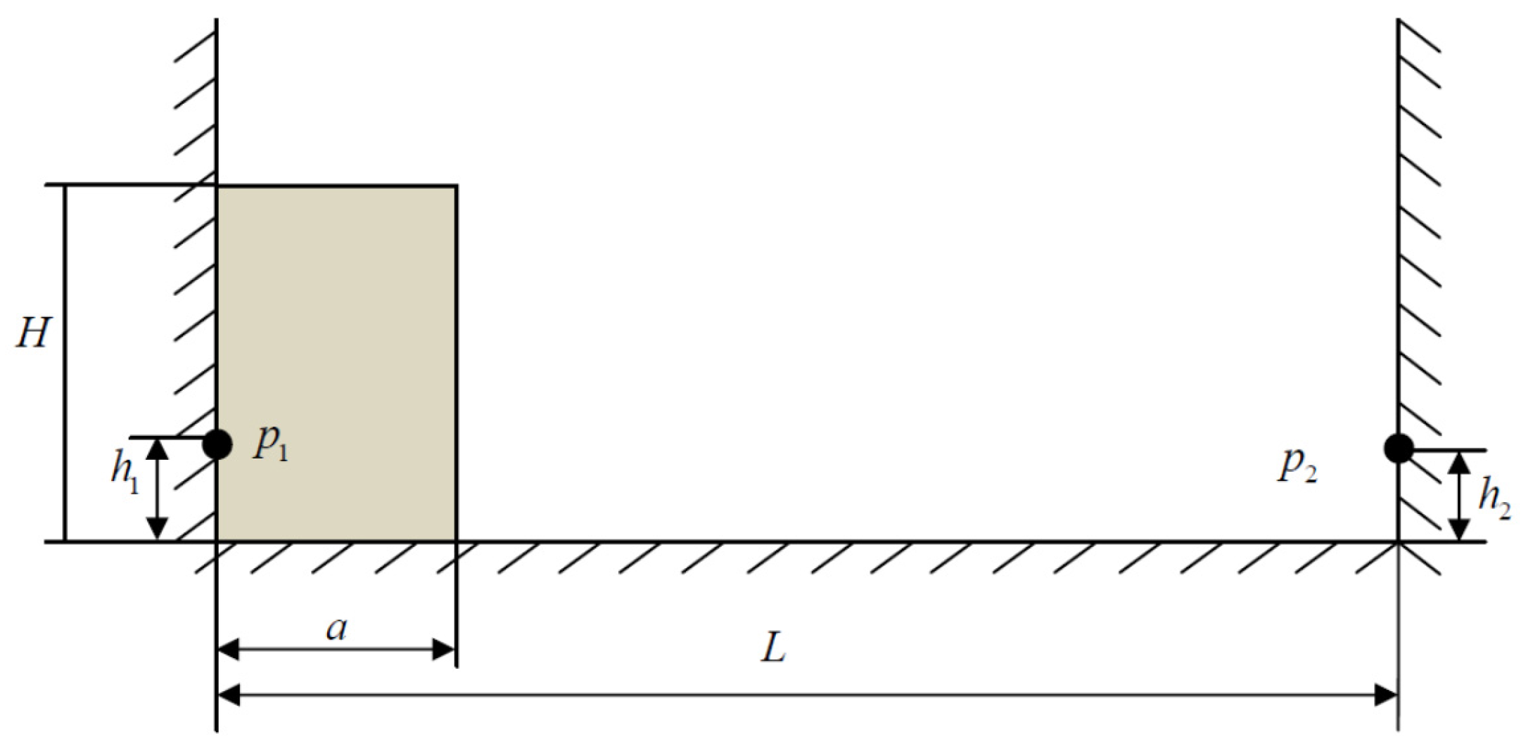
The dam break flow has always been a benchmark violent free surface flow to validate the numerical models. In this example, a rectangular column of water is initially confined. The width of water column is and the height is . At the beginning of the computation, the dam is instantaneously collapsed. A schematic setup of the dam break flow domain is given in Figure 4, where is the distance between the two vertical walls. There are two pressure sensors and located on the left and right walls, respectively, with a distance of and from the horizontal bed. In the following analysis, all the variables are non-dimensionalised by using the dam width and gravitational acceleration , such as or .
In the present simulations it is assumed = 0.5 m, and . The total particle number is 60 × 120 with a particle size of 0.00833 m. The non-dimensionalised time step is given by . To validate the proposed C1_KI SPH computations, Figure 5a,b gives the comparisons of dam break flow leading edge and water column height, respectively, with the experimental results from [28]. A good agreement is found in both cases.
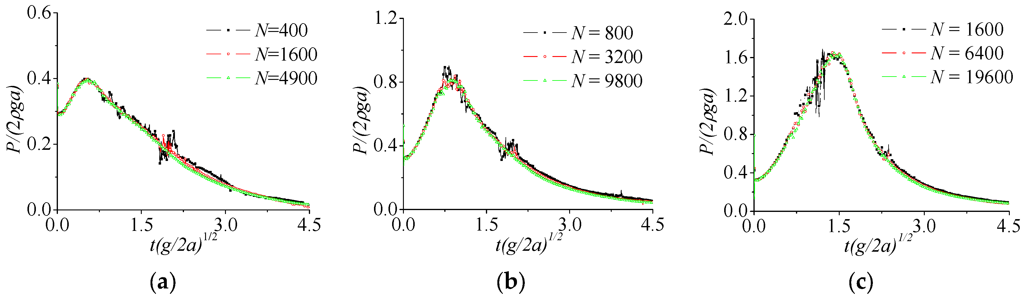
To carry out more robust model validations, three tests are run by changing the height of dam with , and , and the simulations continue to the stage when the dam break wave front hits on the right vertical wall. For analysis purpose, the non-dimensional pressure is expressed as . The total particle numbers used in case of are 400, 1600, 4900, in are 800, 3200, 9800, and in are 1600, 6400, 19600, respectively, for the study of the model convergence. Correspondingly, the particle sizes of three cases are 0.025 m, 0.0125 m and 0.00714 m.
The computational results of pressure time history on sensor point are shown in Figure 6a–c for the different dam height to width ratios . The vertical height of sensor point is from the bed. Figure 6 shows that the peak pressure value changes with the height of water column, which is 0.4, 0.8 and 1.6, respectively, for = 1, 2 and 4. Thus the relationship between maximum pressure and water column height seems to follow a linear correlation. Besides, C1_KI SPH computations demonstrate good convergence behaviours and different particle numbers lead to almost identical results. Although the numerical results demonstrate some kinds of oscillation in the time history, they tend to become smoother with the refinement of particle size.
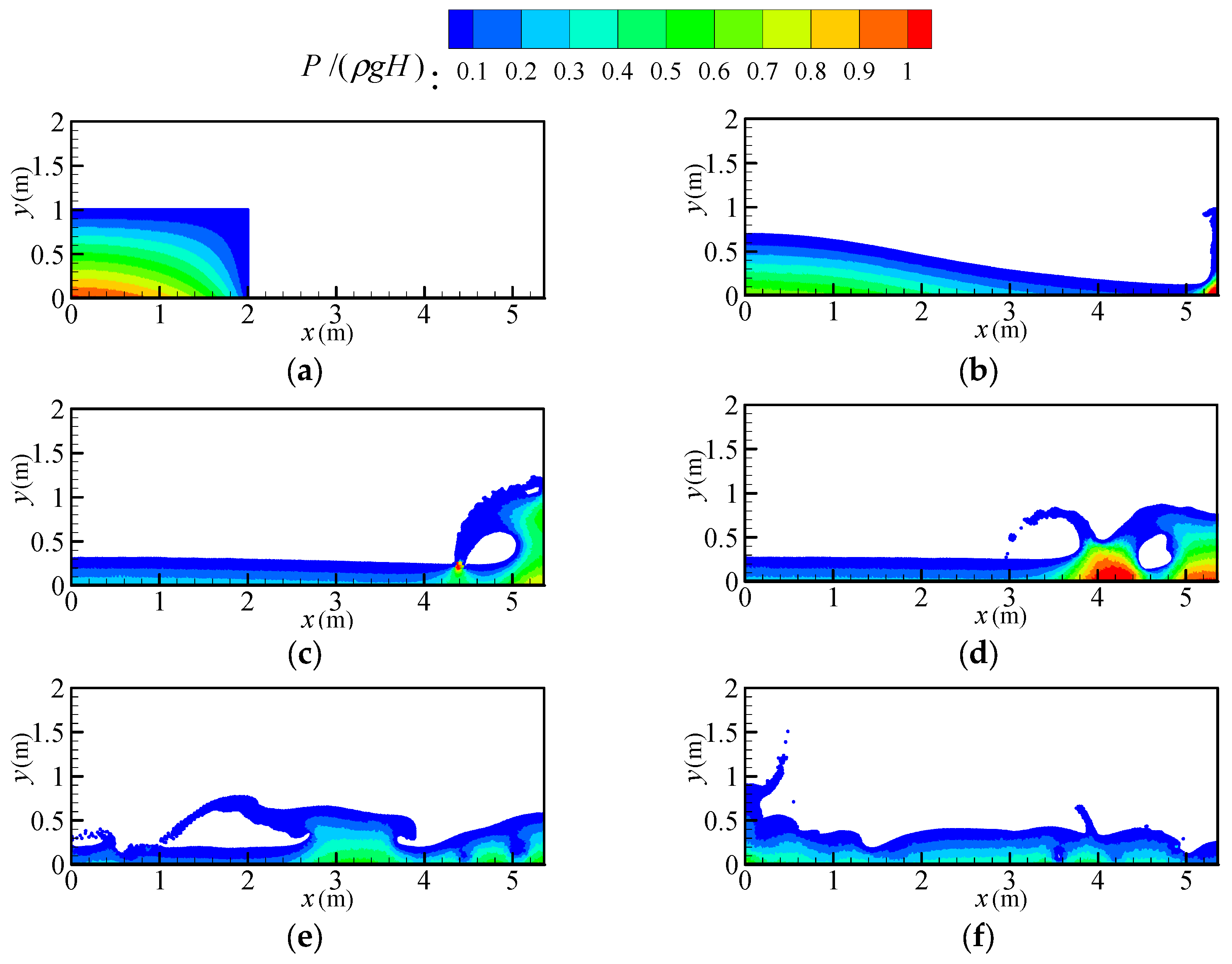
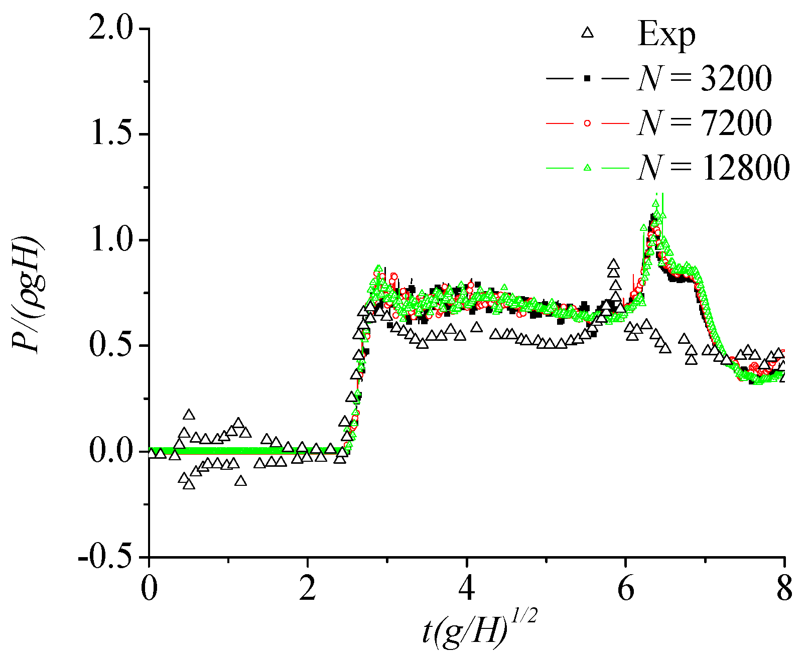
To quantify the accuracy of pressure predictions made by C1_KI SPH, the comparisons with experimental data of Zhou et al. [29] are also made. In this case, the water column dimension is = 2 m and , and the distance between the two vertical walls is . On the right wall, there is a pressure sensor point with a height of from the bed. From the C1_KI SPH simulations, the particle snapshots with pressure distributions are shown in Figure 7a-f at different time instants after the dam break. Besides, Figure 8 gives the time history of dam break flow impact pressures on the right wall computed by using different particle numbers. Compared with the experimental pressure data [29], not only a good agreement has been found, but also the pressure history of C1_KI SPH computations becomes more reasonable with a higher particle resolution.
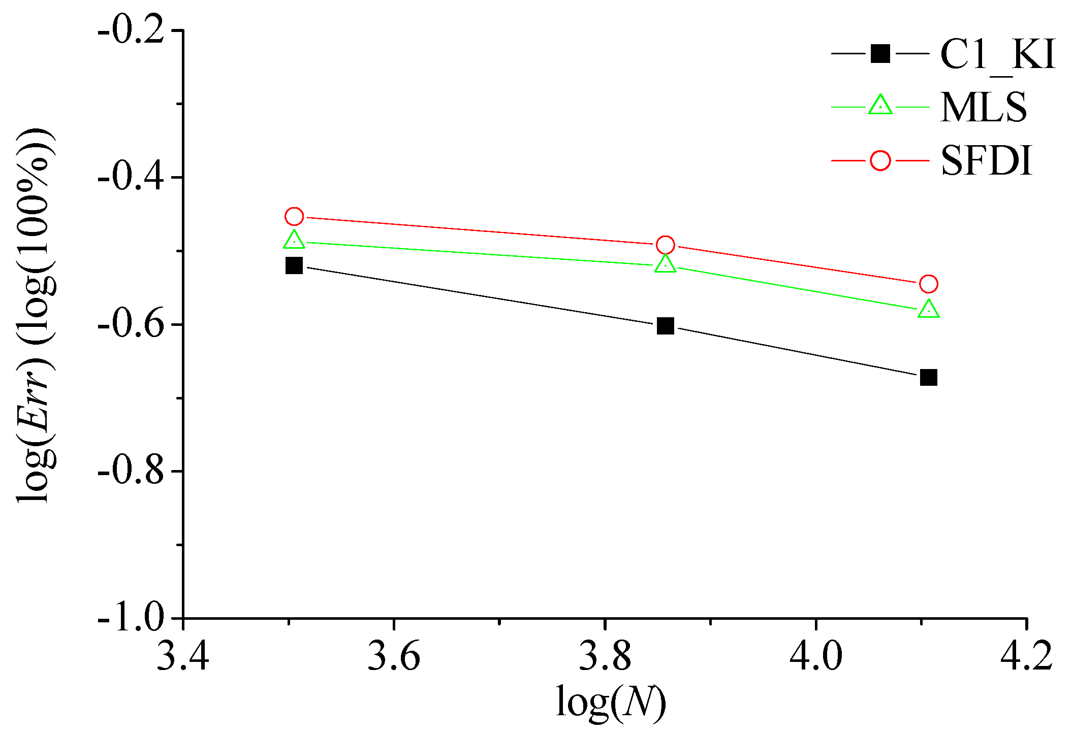
To show more clearly the improvement of proposed model, Figure 9 gives the pressure errors between the experimental data [29] and ISPH results computed by C1_KI, MLS and SFDI models using different particle numbers N. Again it fully demonstrates that C1_ KI scheme can achieve the lowest error and have the fastest convergence rate.
5.2. Solitary Wave Propagation over a Constant Depth
Recently the correlation in between the energy conservation properties and applied pressure gradient models has been extensively explored [30]. The solitary wave propagation over a constant water depth is considered in this section. The interaction between tsunami wave and coastal structure is the topic related to practical coastal and ocean engineering problems and therefore attracts increasing attentions. In most cases, the solitary wave is used to represent certain characteristics of the tsunami wave [31,32]. Long-distance wave propagation is still a huge challenge to SPH models since the wave form cannot be well reserved due to the particle disorders and numerical dissipations. To verify the robustness of the proposed C1_KI SPH scheme, the computed solitary wave profiles are compared with the analytical solutions derived from the Boussinesq equation referred to Zheng et al. [33].
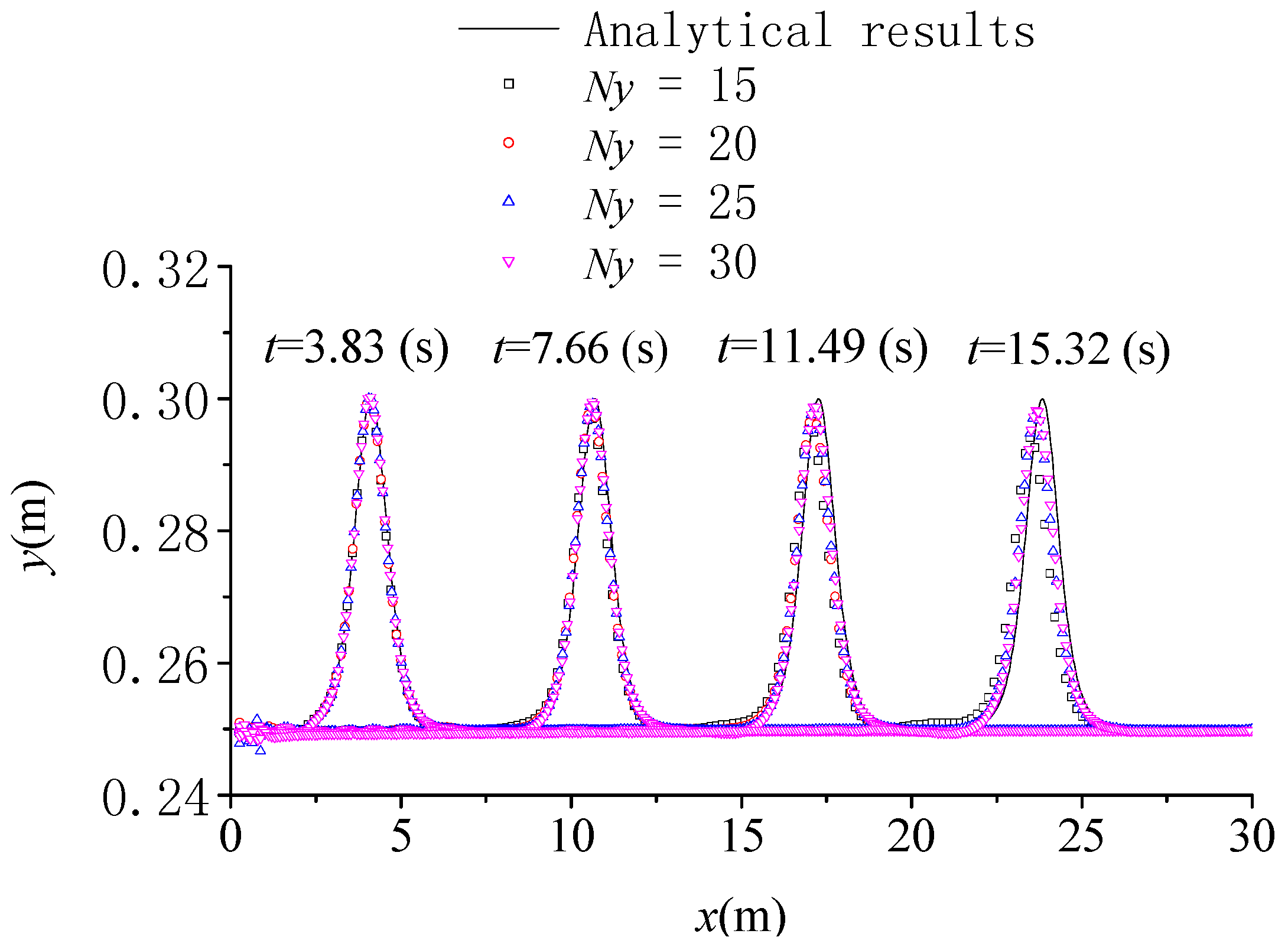
Here, consider a solitary wave with the wave amplitude = 0.05 m, water depth = 0.25 m and total length of the tank = 30.0 m. The computational time step is kept constant as 0.001 s. The numerical solitary wave is generated by a piston-type wave maker according to the theory given in [34], in which the motion of wave maker is defined in a dimensionless form by , and with the dimensionless wave celerity . Figure 10 shows the computed free surface profiles with the analytical solutions for different particle numbers at different times of the wave propagation. It shows that the numerical wave surfaces approach to the analytical ones with the increasing particle number in vertical direction . Meanwhile, the convergence of model computations is evidenced by the close agreement among the three numerical results. Especially it is promising to note that both the wave height and wave shape are well maintained during the wave propagation even if the wave has travelled nearly 30 m over a water depth of 0.25 m. This implies that the dampening of wave height over long-distance travel could be attributed to the influence of pressure gradient calculation schemes. Moreover, in addition to the possible numerical dissipations it has also been shown in the literature that some functions to reproduce the solitary waves lead to a progressive decay in the wave amplitude along the channel as well as the presence of trailing waves due to instantaneous truncation in the motion law of the wave maker. Finally, to show the model convergence more clearly, Figure 11 gives the errors of wave surface elevation between C1_KI SPH results computed with different particle numbers and the analytical results at time = 15.32 s.
5.3. Solitary Wave Impacting on Vertical and Inclined Walls
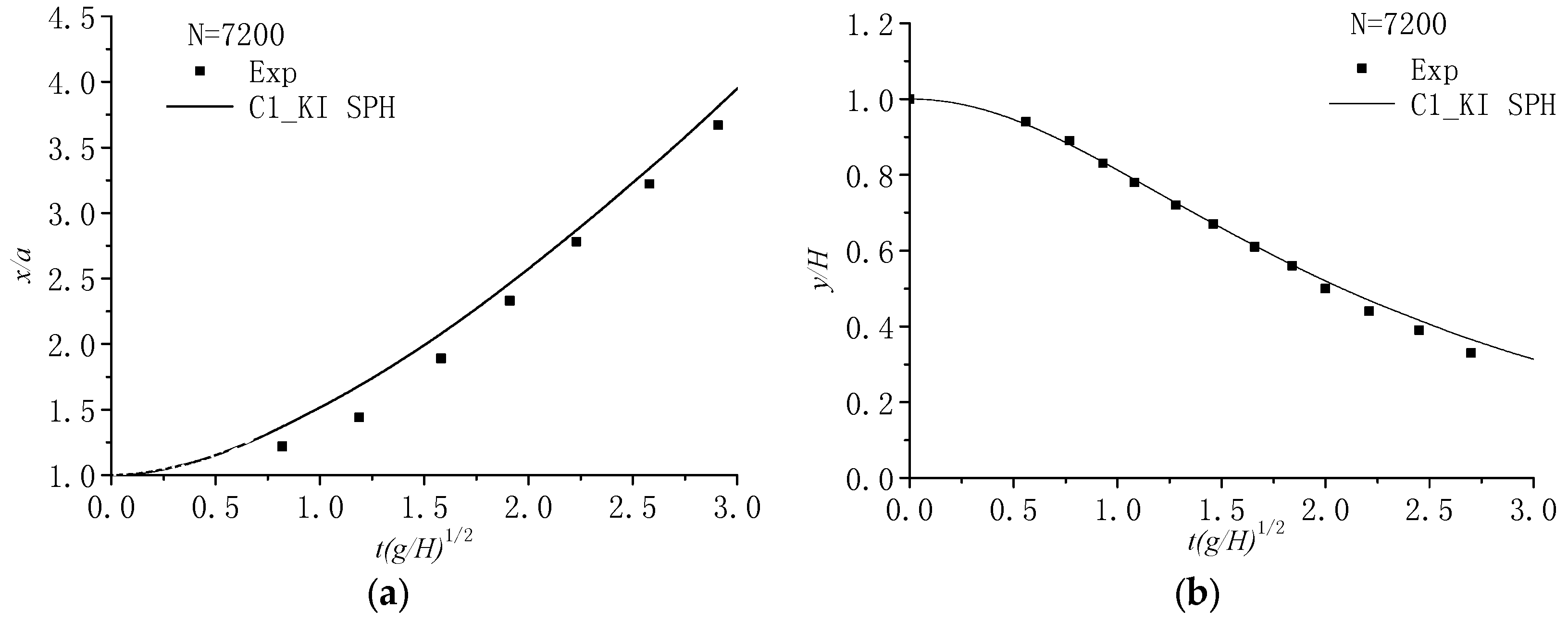
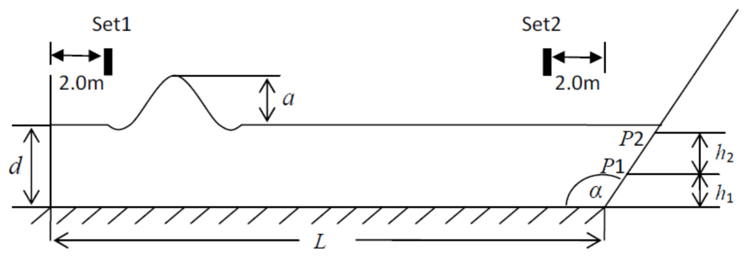
In order to further show the effectiveness of improved C1_KI SPH technique, an investigation is made on the numerical results of a solitary wave propagation and impact on a solid wall with different inclination angles. The physical experiment was carried out by Zheng et al. [35] in a 3-D wave flume with piston wave maker in Harbin Engineering University (HEU). The schematic diagram of the wave tank is shown in Figure 12. The wave tank length is L = 10 m and the water depth is = 0.25 m. The solitary wave height is = 0.15 m and the wave nonlinearity is = 0.6. As shown in Figure 12, two pressure sensor points are located on the right wall at a distance of 0.05 m and 0.15 m from the tank bottom to monitor the pressure time history, i.e., 0.05 m and 0.10 m. Besides, two wave elevation gauges are located at section of Set1 and Set2, which are 2.0 m away from the left and right boundaries, respectively. In the C1_KI SPH computations, the initial particle spacing is chosen to be 0.01 m and the time step is kept constant as 0.001 s.
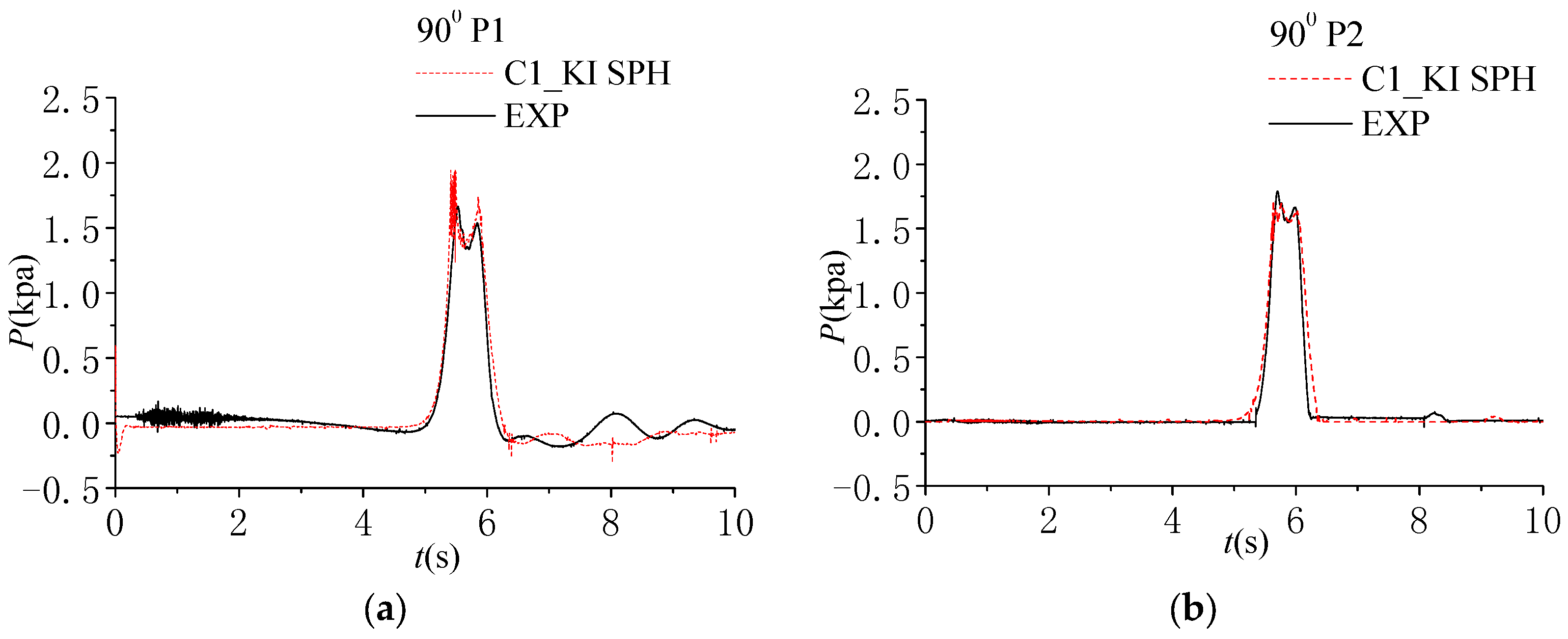
Figure 13a,b gives the comparison of wave surface elevations at Set1 and Set2, and Figure 14a,b gives the comparison of pressure time histories at P1 and P2, for the slope inclination angle = 90°. In order to show the pressure time histories more clearly, only the dynamic parts of the pressures are provided, while the total pressure should be obtained by adding to the part of static pressure. From the results in both figures, it shows that C1_KI SPH computations can achieve good results as compared with the experimental data [35]. Since there is a reflected wave after the solitary wave impacts on the slope, it shows double peaks in the wave elevation time history at Set2 in Figure 13. Due to the wave running up and down, there are some discrepancies in the numerical results after the solitary wave reflects from the slope. The pressure time histories at point P1 in Figure 14 are not as good as those at point P2, as there are some small oscillations in the peak domain. This is due to that some small water drops hit upon the water surface and make the pressure of inner particles change rapidly. The pressure amplitude at P1 and P2 are almost the same. It should be noted that the double peak pressure patterns in Figure 14 have also been reported in a latest ISPH work [36].
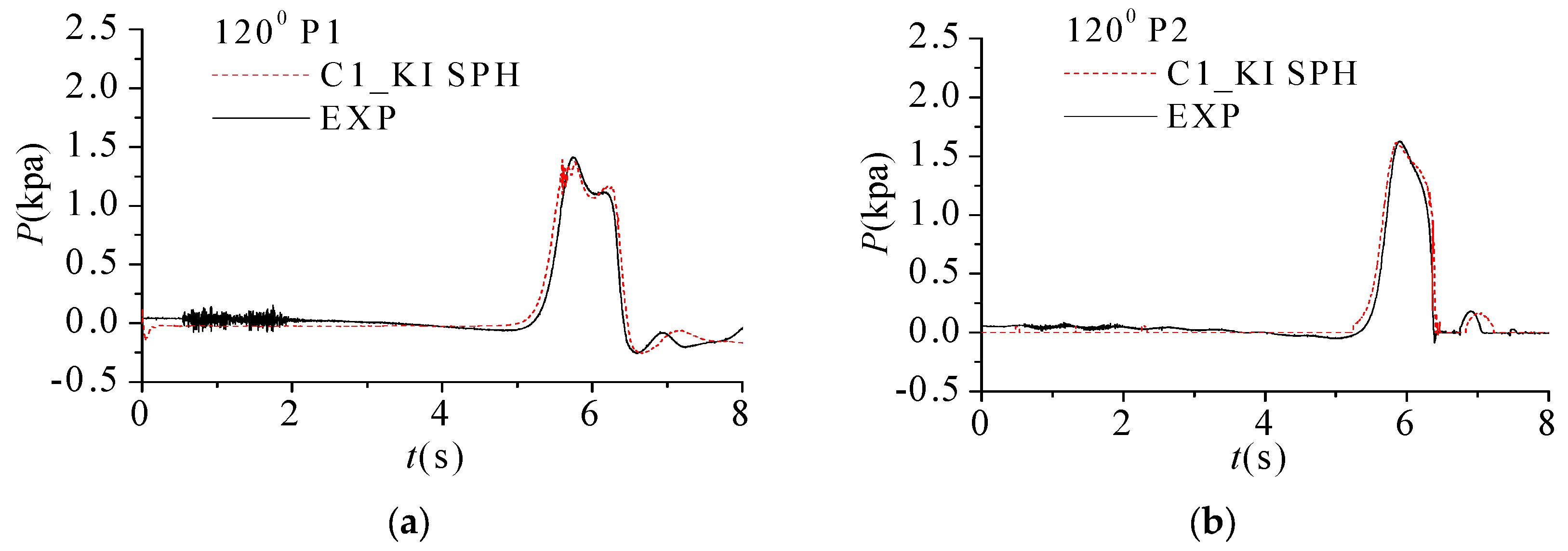
For generality, Figure 15a,b and Figure 16a,b give the comparisons of wave surface elevations at Set1 and Set2, and time histories of wave impact pressures at P1 and P2, respectively, when the slope angle is = 120°. As there exist the overturning and re-entering waves, the amplitude of reflected waves becomes smaller than the case of Figure 13. Due to being difficult to simulate the air-pocket and small bubbles in present model, the amplitude and phase of waves demonstrate some differences between the experimental data [35] and numerical ISPH results. With the increase of slope inclinations, i.e., from = 90° to = 120°, the amplitude of reflected wave elevations and wave impact pressures becomes smaller, and the duration of wave impact becomes longer, following the comparisons between Figure 13 and Figure 15, or between Figure 14 and Figure 16. Due to the 3D effect of wave propagation and small vibrations from the piston wave maker, there is a phenomenon of trailing waves appearing in Figure 13a and Figure 15a.
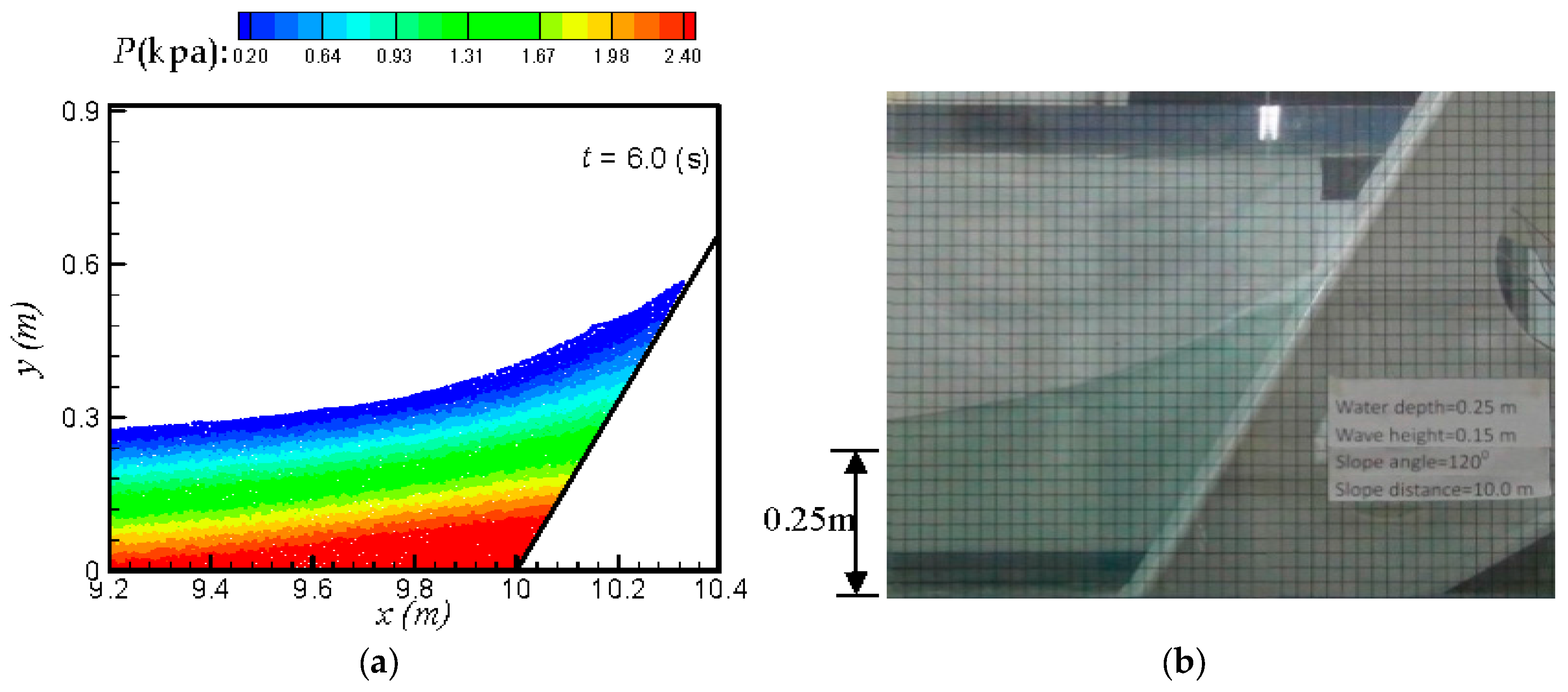
Finally, Figure 17a,b gives a snapshot of the computed wave profile with the experimental photo at time = 6 s, including the pressure contour distributions in the fluid domain. It shows again that the wave elevation profile obtained by C1_KI SPH can achieve a good agreement with the laboratory photograph, and the pressure distribution of wave field is quite stable and noise-free.
6. Conclusions and Discussions
An improved ISPH method is proposed to simulate violent water wave propagation and impact upon coastal structures such as vertical and inclined walls. After the comparisons of different first-order derivative calculation models, such as SFDI, MLS and C1_KI, C1_KI SPH has found to perform the best considering both the inner fluid domain and the near boundary region when the particles are randomly distributed. In practical model applications, the results of dam break flow computed by C1_KI SPH show good agreement with the experimental data. Then the robustness of C1_KI SPH is further verified by the solitary wave propagation over a long-distance with almost no wave height dampening, which implies that the accurate pressure calculation could be the key issues in modelling of wave system. Finally, the model is applied to the solitary wave impact on a slope with different orientation angles. After compared with the experimental data for two different slopes angles, i.e., 90° and 120°, the computational results of C1_KI SPH demonstrate its great potential in predicting the wave surface elevations and impact pressures in water wave system.
The main contributions of the paper lie in the following aspects: Firstly, it proposes the improved numerical scheme of C1_KI, which effectively avoids the process of kernel gradient calculation. The relevant matrix is strictly in symmetric distribution, so only the upper triangle elements need to be calculated while others can be obtained from the symmetric relationship. Secondly, a comprehensive analysis of SFDI, MLS and C1_KI benchmarks indicated that the proposed one achieves the most accuracy regardless of whether the particles are regularly or irregularly distributed in the inner fluid area. Considering the solid boundary effect, the accuracy of C1_KI is comparable with that of the existing approaches, but its numerical scheme is more straightforward in terms of the formulation and is more efficient in terms of CPU time costs. Thirdly, it is the first time that C1_KI scheme and truly incompressible SPH are combined for the water wave propagation and impact simulations, which has been evidenced by the high accuracy results and low dissipations of the wave peaks as well as stable pressure distributions.
Acknowledgments
This research work is supported by the National Natural Science Foundation of China (Nos. 51009034, 51279041, 51379051, 51479087 and 51639004), Foundational Research Funds for the Central Universities (Nos. HEUCDZ1202 and HEUCF170104) and Defence Pre Research Funds Program (No. 9140A14020712CB01158), to which the authors are most grateful. Author Q. Ma also thanks the Chang Jiang Visiting Chair Professorship Scheme of the Chinese Ministry of Education, hosted by HEU.
Author Contributions
All authors contributed to the work. X. Zheng performed the computations and data analysis; Q. Ma guided the engineering project and provided the data; S. Shao proofread and edited the manuscript; and A. Khayyer proofread and commented on the manuscript.
Conflicts of Interest
The authors declare no conflict of interest.
References
- Grilli, S.T.; Guyenne, P.; Dias, F. A fully nonlinear model for three-dimensional overturning waves over arbitrary bottom. Int. J. Numer. Methods Fluids 2001, 35, 829–867. [Google Scholar] [CrossRef]
- Celebi, M.S.; Kim, M.H.; Beck, R.F. Fully nonlinear 3D numerical wave tank simulation. J. Ship Res. 1998, 42, 33–45. [Google Scholar]
- Ma, Q.W.; Wu, G.X.; Eatock Taylor, R. Finite element simulation of fully non-linear interaction between vertical cylinders and steep waves. Part 2: Numerical results and validation. Int. J. Numer. Methods Fluids 2001, 36, 287–308. [Google Scholar] [CrossRef]
- Yue, W.; Lin, C.L.; Patel, V.C. Numerical simulation of unsteady multidimensional free surface motions by level set method. Int. J. Numer. Methods Fluids 2003, 42, 853–884. [Google Scholar] [CrossRef]
- Greaves, D.M. Simulation of interface and free surface flows in a viscous fluid using adaptive quadtree grids. Int. J. Numer. Methods Fluids 2004, 44, 1093–1117. [Google Scholar] [CrossRef]
- Wang, P.; Yao, Y.; Tulin, M. An efficient numerical tank for nonlinear water waves, based on the multi-subdomain approach with BEM. Int. J. Numer. Methods Fluids 1995, 20, 1315–1336. [Google Scholar] [CrossRef]
- Wu, G.X.; Hu, Z.Z. Simulation of nonlinear interactions between waves and floating bodies through a finite-element-based numerical tank. Proc. R. Soc. A 2004, 460, 3037–3058. [Google Scholar] [CrossRef]
- Stansby, P. Solitary wave runup and overtopping by a semi-implicit finite volume shallow-water Boussinesq model. J. Hydraulic Res. 2003, 41, 639–647. [Google Scholar] [CrossRef]
- Lucy, L.B. A numerical approach to the testing of fusion process. Astron. J. 1977, 88, 1013–1024. [Google Scholar] [CrossRef]
- Monaghan, J.J. Simulating free surface flows with SPH. J. Comput. Phys. 1994, 110, 399–406. [Google Scholar] [CrossRef]
- Gomez-Gesteira, M.; Cerqueiroa, D.; Crespo, C.; Dalrymple, R.A. Green water overtopping analyzed with a SPH model. Ocean Eng. 2005, 32, 223–238. [Google Scholar] [CrossRef]
- Koshizuka, S.; Oka, Y. Moving-particle semi-implicit method for fragmentation of incompressible fluid. Nucl. Sci. Eng. 1996, 123, 421–434. [Google Scholar]
- Cummins, S.J.; Rudman, M. An SPH projection method. J. Comput. Phys. 1999, 152, 584–607. [Google Scholar] [CrossRef]
- Shao, S.D.; Lo, E.Y.M. Incompressible SPH method for simulating Newtonian and non-Newtonian flows with a free surface. Adv. Water Resour. 2003, 26, 787–800. [Google Scholar] [CrossRef]
- Khayyer, A.; Gotoh, H.; Shao, S.D. Corrected incompressible SPH method for accurate water-surface tracking in breaking waves. Coast. Eng. 2008, 55, 236–250. [Google Scholar] [CrossRef]
- Crespo, A.J.C.; Dominguez, J.M.; Rogers, B.D.; Gómez-Gesteira, M.; Longshaw, S.; Canelas, R.; Vacondio, R.; Barreiro, A.; García-Feal, O. DualSPHysics: Open-source parallel CFD solver based on Smoothed Particle Hydrodynamics (SPH). Comput. Phys. Commun. 2015, 187, 204–216. [Google Scholar] [CrossRef]
- Aristodemo, F.; Meringolo, D.D.; Groenenboom, P.; Lo Schiavo, A.; Veltri, P.; Veltri, M. Assessment of dynamic pressures at vertical and perforated breakwaters through diffusive SPH schemes. Math. Probl. Eng. 2015, 2015, 305028. [Google Scholar] [CrossRef]
- Meringolo, D.D.; Aristodemo, F.; Veltri, P. SPH numerical modeling of wave-perforated breakwater interaction. Coast. Eng. 2015, 101, 48–68. [Google Scholar] [CrossRef]
- Meringolo, D.D.; Colagrossi, A.; Marrone, S.; Aristodemo, F. On the filtering of acoustic components in weakly-compressible SPH simulations. J. Fluids Struct. 2017, 70, 1–23. [Google Scholar] [CrossRef]
- Marrone, S.; Colagrossi, A.; Di Mascio, A.; Le Touzé, D. Prediction of energy losses in water impacts using incompressible and weakly compressible models. J. Fluids Struct. 2015, 54, 802–822. [Google Scholar] [CrossRef]
- Zheng, X.; Ma, Q.W.; Duan, W.Y. Comparative study of different SPH schemes on simulating violent water wave impact flows. China Ocean Eng. 2014, 28, 791–806. [Google Scholar] [CrossRef]
- Zheng, X.; Ma, Q.W.; Duan, W.Y. Incompressible SPH method based on Rankine source solution for violent water wave simulation. J. Comput. Phys. 2014, 276, 291–314. [Google Scholar] [CrossRef]
- Sriram, V.; Ma, Q.W. Improved MLPG_R method for simulating 2D interaction between violent waves and elastic structures. J. Comput. Phys. 2012, 231, 7650–7670. [Google Scholar] [CrossRef]
- Ma, Q.W. A new meshless interpolation scheme for MLPG_R method. CMES Comput. Model. Eng. Sci. 2008, 23, 75–89. [Google Scholar]
- Aturi, S.N.; Shen, S. The Meshless Local Petrove-Galerkin (MLPG) method: A simple & less-costly alternative to the finite element and boundary element methods. CMES Comput. Model. Eng. Sci. 2002, 3, 11–52. [Google Scholar]
- Zheng, X.; Duan, W.Y.; Ma, Q.W. Comparison of improved meshless interpolation schemes for SPH method and accuracy analysis. Int. J. Mar. Sci. Appl. 2010, 9, 223–230. [Google Scholar] [CrossRef]
- Yang, J.Y.; Zhao, Y.M.; Liu, N.; Bu, W.P.; Xu, T.L.; Tang, Y.F. An implicit MLS meshless method for 2-D time dependent fractional diffusion-wave equation. Appl. Math. Model. 2015, 39, 1229–1240. [Google Scholar] [CrossRef]
- Martin, J.C.; Moyce, W.J. Part IV. An experimental study of the collapse of liquid columns on a rigid horizontal plane. Philos. Trans. R. Soc. Lond. Ser. A Math. Phys. Sci. 1952, 244, 312–324. [Google Scholar] [CrossRef]
- Zhou, Z.Q.; De Kat, J.O.; Buchner, B. A nonlinear 3-D approach to simulate green water dynamics on deck. In Proceedings of the 7th International Conference on Numerical Ship Hydrodynamics, Nantes, France, 19–22 July 1999; pp. 1–15. [Google Scholar]
- Khayyer, A.; Gotoh, H.; Shimizu, Y.; Gotoh, K. On enhancement of energy conservation properties of projection-based particle methods. Eur. J. Mech. B/Fluids 2017, in press. Available online: http://dx.doi.org/10.1016/j.euromechflu.2017.01.014 (accessed on 3 June 2017).
- Liang, D.F.; Thusyanthan, I.; Madabhushi, S.P.G.; Tang, H. Modelling solitary waves and its impact on coastal houses with SPH method. China Ocean Eng. 2010, 24, 353–368. [Google Scholar]
- Lin, P.Z.; Liu, X.; Zhang, J. The simulation of a landside-induced surge wave and its overtopping of a dam using a coupled ISPH model. Eng. Appl. Comput. Fluid Mech. 2015, 9, 432–444. [Google Scholar]
- Zheng, X.; Shao, S.D.; Khayyer, A.; Duan, W.Y.; Ma, Q.W.; Liao, K.P. Corrected first-order derivative ISPH in water wave simulations. Coast. Eng. J. 2017, 59, 1750010. [Google Scholar] [CrossRef]
- Ma, Q.W.; Zhou, J. MLPG_R method for numerical simulation of 2D breaking waves. CMES Comput. Model. Eng. Sci. 2009, 43, 277–304. [Google Scholar]
- Zheng, X.; Hu, Z.H.; Ma, Q.W.; Duan, W.Y. Incompressible SPH based on rankine source solution for water wave impact simulation. Procedia Eng. 2015, 126, 650–654. [Google Scholar] [CrossRef]
- Liang, D.F.; Jian, W.; Shao, S.D.; Chen, R.D.; Yang, K.J. Incompressible SPH simulation of solitary wave interaction with movable seawalls. J. Fluids Struct. 2017, 69, 72–88. [Google Scholar] [CrossRef]
Figure 1.
Random particle distributions with particle number: (a) 400; (b) 1600; (c) 6400; and (d) 25,600.
Figure 1.
Random particle distributions with particle number: (a) 400; (b) 1600; (c) 6400; and (d) 25,600.

Figure 2.
Convergence and error analysis of first-order derivative calculation under uniform particle distributions in the: (a) inner fluid area; and (b) near boundary area.
Figure 2.
Convergence and error analysis of first-order derivative calculation under uniform particle distributions in the: (a) inner fluid area; and (b) near boundary area.

Figure 3.
Convergence and error analysis of first-order derivative calculation under disordered particle distributions in the: (a) inner fluid area; and (b) near boundary area.
Figure 3.
Convergence and error analysis of first-order derivative calculation under disordered particle distributions in the: (a) inner fluid area; and (b) near boundary area.

Figure 4.
Schematic setup of dam break flow domain.

Figure 5.
Comparisons between C1_KI SPH computations and experimental results on dam break flow: (a) leading edge; and (b) water column height.
Figure 5.
Comparisons between C1_KI SPH computations and experimental results on dam break flow: (a) leading edge; and (b) water column height.

Figure 6.
Time history of computed pressures for different water column height and particle number: (a) ; (b) ; and (c) .
Figure 6.
Time history of computed pressures for different water column height and particle number: (a) ; (b) ; and (c) .

Figure 7.
Particle snapshots with pressure distributions at different times computed by C1_KI SPH: (a) = 0.0; (b) = 3.0; (c) = 6.0; (d) = 6.75; (e) = 9.0; and (f) = 12.0.
Figure 7.
Particle snapshots with pressure distributions at different times computed by C1_KI SPH: (a) = 0.0; (b) = 3.0; (c) = 6.0; (d) = 6.75; (e) = 9.0; and (f) = 12.0.

Figure 8.
Pressure time history on right wall computed by C1_KI SPH with different particle numbers, compared with experimental data [29].
Figure 8.
Pressure time history on right wall computed by C1_KI SPH with different particle numbers, compared with experimental data [29].

Figure 9.
Comparisons of pressure errors for C1_KI, MLS and SFDI models with different particle numbers.
Figure 9.
Comparisons of pressure errors for C1_KI, MLS and SFDI models with different particle numbers.

Figure 10.
Comparisons of wave surface profile computed by C1_KI SPH using different particle resolutions with analytical solutions at different wave propagation stages.
Figure 10.
Comparisons of wave surface profile computed by C1_KI SPH using different particle resolutions with analytical solutions at different wave propagation stages.

Figure 11.
Convergence study of wave surface elevations computed by C1_KI SPH with different particle resolutions.
Figure 11.
Convergence study of wave surface elevations computed by C1_KI SPH with different particle resolutions.
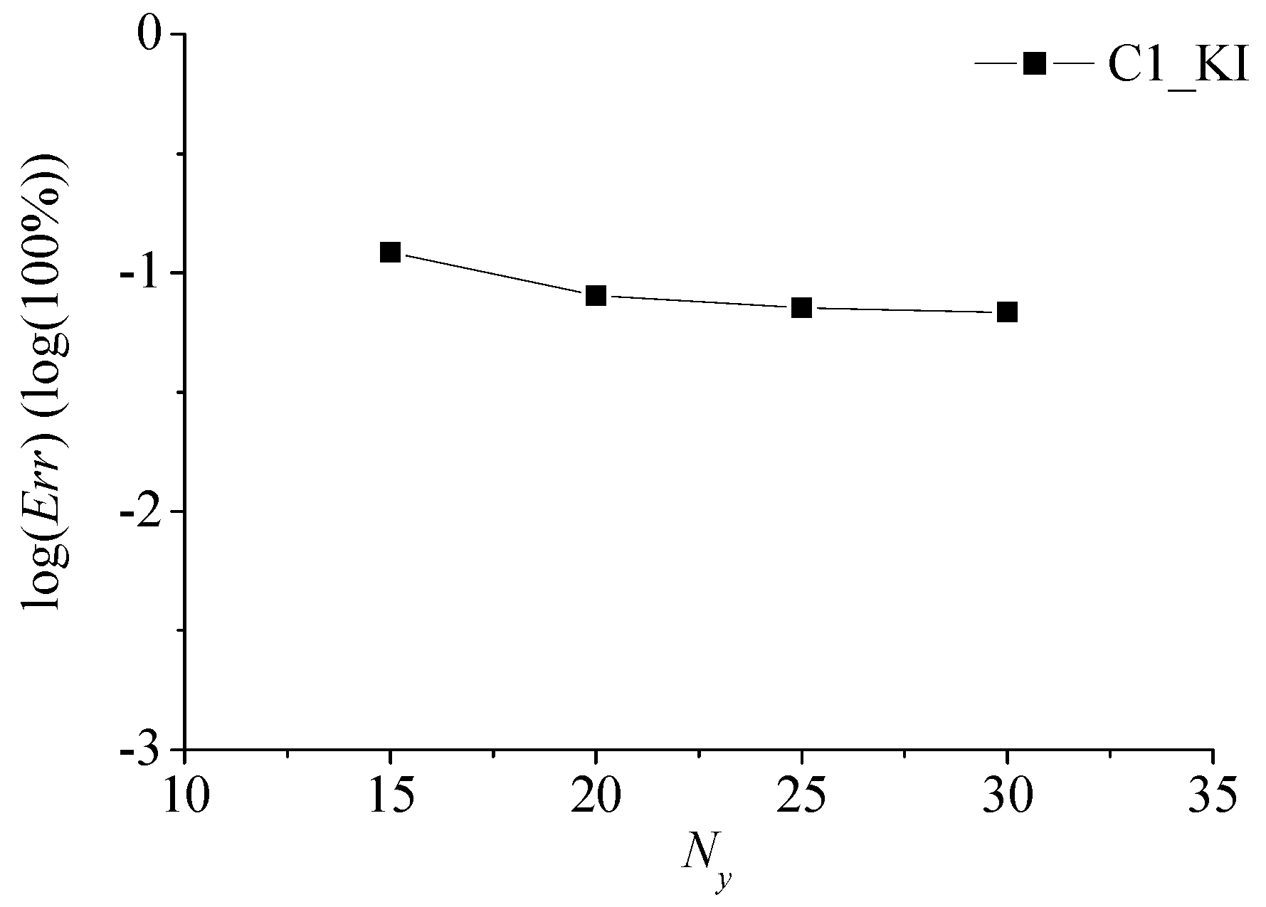
Figure 12.
Schematic view of solitary wave tank and measurement locations.

Figure 13.
Comparisons of wave surface elevations computed by C1_KI SPH with experimental data [35] for slope angle 90° at: (a) Set1; and (b) Set2.
Figure 13.
Comparisons of wave surface elevations computed by C1_KI SPH with experimental data [35] for slope angle 90° at: (a) Set1; and (b) Set2.
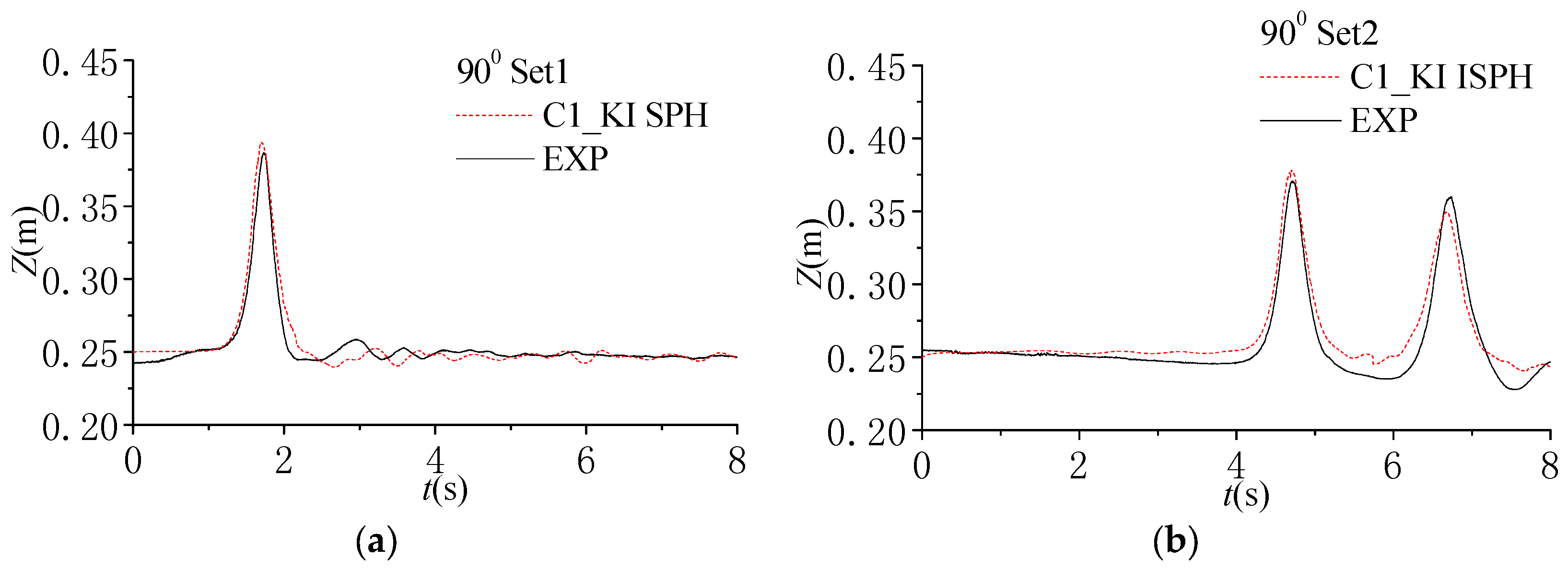
Figure 14.
Comparisons of wave impact pressure time histories computed by C1_KI SPH with experimental data [35] for slope angle 90° at: (a) P1; and (b) P2.
Figure 14.
Comparisons of wave impact pressure time histories computed by C1_KI SPH with experimental data [35] for slope angle 90° at: (a) P1; and (b) P2.

Figure 15.
Comparisons of wave surface elevations computed by C1_KI SPH with experimental data [35] for slope angle 120° at: (a) Set1; and (b) Set2.
Figure 15.
Comparisons of wave surface elevations computed by C1_KI SPH with experimental data [35] for slope angle 120° at: (a) Set1; and (b) Set2.
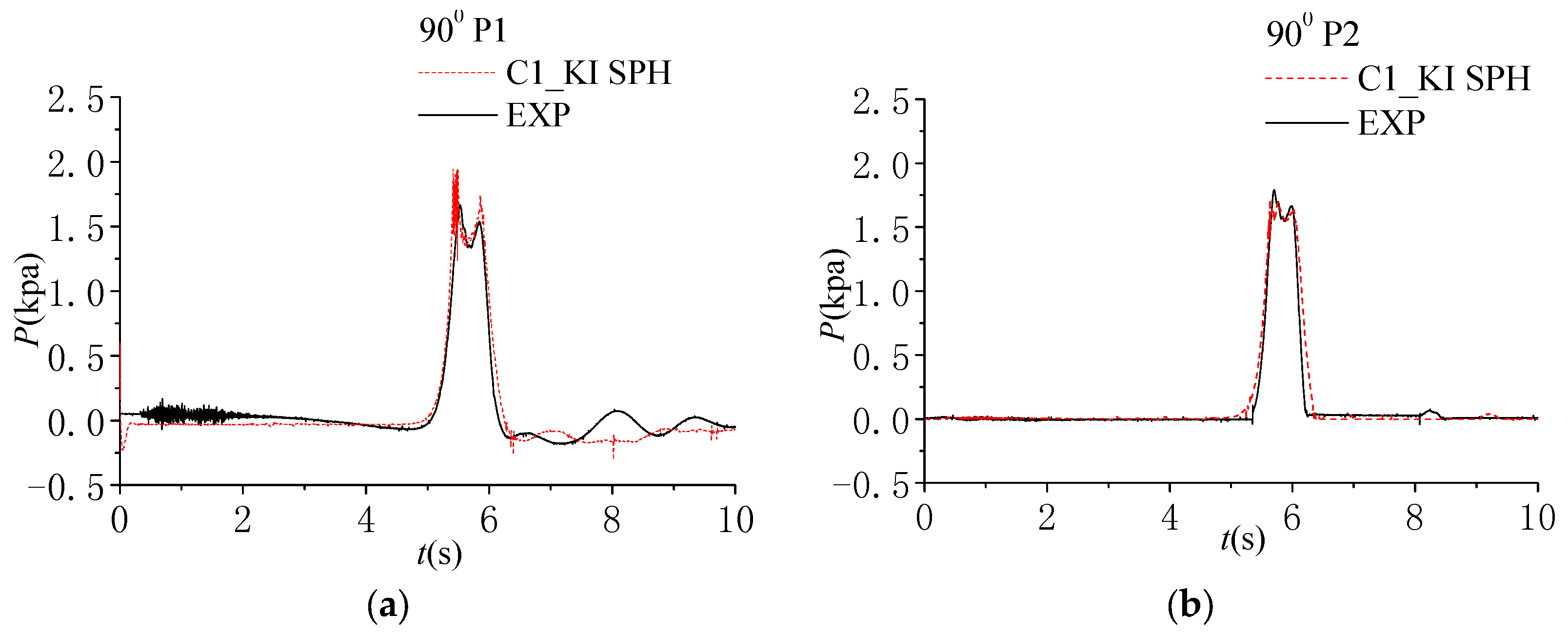
Figure 16.
Comparisons of wave impact pressure time histories computed by C1_KI SPH with experimental data [35] for slope angle 120° at: (a) P1; and (b) P2.
Figure 16.
Comparisons of wave impact pressure time histories computed by C1_KI SPH with experimental data [35] for slope angle 120° at: (a) P1; and (b) P2.

Figure 17.
Wave surface profile during its run-up at t = 6 s, compared between: (a) C1_KI SPH computations; and (b) Laboratory photograph.
Figure 17.
Wave surface profile during its run-up at t = 6 s, compared between: (a) C1_KI SPH computations; and (b) Laboratory photograph.
© 2017 by the authors. Licensee MDPI, Basel, Switzerland. This article is an open access article distributed under the terms and conditions of the Creative Commons Attribution (CC BY) license (http://creativecommons.org/licenses/by/4.0/).
Share and Cite
MDPI and ACS Style
Zheng, X.; Ma, Q.; Shao, S.; Khayyer, A. Modelling of Violent Water Wave Propagation and Impact by Incompressible SPH with First-Order Consistent Kernel Interpolation Scheme. Water 2017, 9, 400. https://doi.org/10.3390/w9060400
AMA Style
Zheng X, Ma Q, Shao S, Khayyer A. Modelling of Violent Water Wave Propagation and Impact by Incompressible SPH with First-Order Consistent Kernel Interpolation Scheme. Water. 2017; 9(6):400. https://doi.org/10.3390/w9060400
Chicago/Turabian StyleZheng, Xing, Qingwei Ma, Songdong Shao, and Abbas Khayyer. 2017. "Modelling of Violent Water Wave Propagation and Impact by Incompressible SPH with First-Order Consistent Kernel Interpolation Scheme" Water 9, no. 6: 400. https://doi.org/10.3390/w9060400
Note that from the first issue of 2016, this journal uses article numbers instead of page numbers. See further details here.