Abstract
Meteorological drought monitoring is important for drought early warning and disaster prevention. Regional meteorological drought can be evaluated and analyzed with standardized precipitation index (SPI). Two main processing schemes are frequently adopted: (1) mean of all SPI calculated from precipitation at individual stations (SPI-mean); and (2) SPI calculated from all-station averaged precipitation (precipitation-mean). It yet remains unclear if two processing schemes could make difference in drought assessment, which is of significance to reliable drought monitoring. Taking the Poyang Lake Basin with monthly precipitation recorded by 13 national stations for 1957–2014, this study examined two processing schemes. The precipitation mean and SPI mean were respectively calculated with the Thiessen Polygon weighting approach. Our results showed that the two SPI series individually constructed from two schemes had similar features and monitoring trends of regional meteorological droughts. Both SPI series had a significantly positive correlation (p < 0.005) with the number of precipitation stations. The precipitation-mean scheme reduced the extent of precipitation extremes and made the precipitation data more clustered in some certain, it made less precipitation deviate from the precipitation-mean series farther when less precipitation occurred universally, which would probably change the drought levels. Alternatively, the SPI-mean scheme accurately highlighted the extremes especially for those with wide spatial distribution over the region. Therefore, for regional meteorological drought monitoring, the SPI-mean scheme is recommended for its more suitable assessment of historical droughts.
1. Introduction
As a hydroclimatic hazard, drought poses a serious threat to society, economy, ecosystem and other sectors [1,2]. The droughts have been increasing worldwide [3,4]. Droughts occur in any climate zone, and their properties (frequency, duration, and severity) may differ from one to another [5]. Quantitative assessment of drought features and its development is essential to understanding different drought types at scales from the local to the global [6]. However, there is currently no general consensus on the definition of drought [4,6,7,8,9,10,11,12], which has been a stumbling block in drought monitoring and analysis. The American Meteorological Society [13] summarized dozens of drought definitions into four categories: meteorological, agricultural, hydrological and socioeconomic droughts. The four categories are associated with different components of hydrologic cycle [14]. Generally, precipitation is the driving and critical factor in the hydrologic cycle. The absence or reduction of precipitation instigates meteorological drought. Subsequently, short-term dryness in the surface and subsurface layers may result in agricultural drought. Finally, when precipitation deficits stay for a prolonged period, low recharge from soil to water features (lakes, groundwater, and rivers) causes a delayed hydrological drought [4,15]. The propagation from meteorological drought to hydrological drought is characterized in terms of pooling, time lag, attenuation, and lengthening [16,17,18]. That is to say, meteorological drought, which is defined as a lack of precipitation over region for a period of time [4], plays an important role in subsequent drought formation and propagation across different drought types [19].
In practice, drought assessment for a specific area is often required for disaster prevention from local agencies or communities [20]. Akhtari et al. [21] pointed out that tracking the droughts in cities is one of the most objectives of drought mapping. Zhang et al. [22] assessed drought vulnerability with SPI taking county as a study unit and the assessment was useful for early warning of regional droughts [23]. The National Temperature and Precipitation Maps of the National Oceanic and Atmospheric Administration’s National Centers for Environmental Information provides the drought products at different scales from national, regional, statewide, and divisional. Hydrologically, the region impacted by drought is not only limited to river network and its vicinity, but also the whole basin [24]. As an elementary unit of hydrologic processes, basin with a high degree of functional integrity contains abundant hydrological information. Basin-scale analysis is beneficial to reveal the interactions among multiple hydrologic variables [25]. Thus, it is highly worthwhile to study meteorological drought at a basin scale.
In recent decades, many drought indices have been proposed, such as Z-index Palmer [8], Palmer Drought Severity Index (PDSI) [8], Standardized Precipitation Index (SPI) [26], Effective Drought Index (EDI) [27], Reconnaissance Drought Index (RDI) [28], Standardized Precipitation Evapotranspiration Index (SPEI) [29]. Among these indices, the SPI has been widely applied in many aspects [3,27,30,31,32,33,34,35,36,37], and recommended as a standard index for tracking meteorological droughts by the World Meteorological Organization [38]. At present, two processing schemes are frequently adopted for regional drought assessment. In the first case, SPI is first calculated from precipitation for each individual stations and then regional SPI is obtained by averaging the SPI values of all the stations (SPI-mean, hereafter, Case A). In the second case, regional precipitation is at first obtained by averaging the precipitation of all the stations and then SPI is calculated from the average precipitation (precipitation-mean, hereafter, Case B). Livada and Assimakopoulos applied the Case-A processing scheme to analyze temporal trend of droughts in Greece [31]. Zhai et al. quantitatively analyzed frequencies of dry and wet years and its tendency for 7 basins and 3 regions in China with the time series of averaged annual SPI [39]. Gao and Zhang used the mean annual SDI and SPI series to disclose a tendency towards wetter condition in the Hexi Corridor, China [40]. Dash et al. investigated the characteristics of meteorological droughts in Bangladesh using SPI obtained with the Case-B scheme [41]. The characteristics (frequency, duration, and severity) of historical drought events based on SPI series obtained from areal mean precipitation are often applied to construct and examine the probabilistic models (using the Case B processing scheme) [42]. For drought assessment of an entire region based on local observations, either of two processing schemes is frequently used. Two processing schemes both involve space average. Hence, the difference between two processing schemes may result from the heterogeneity of precipitation. Furthermore, the mean-precipitation and mean-SPI schemes may produce different SPI values, providing that the local observations are generally not homogeneously distributed [43]. There are few studies to compare two processing schemes, leaving a gap for users to select a suitable scheme for reliable assessment of regional droughts.
The areal SPI values are the crucial basis and input variables for drought evolution, regional drought vulnerability assessment, and drought quantitative models. Therefore, the reasonable areal SPI series are of great importance. However, the different processing schemes might result in the dissimilar estimation results. Thus, this study uses both processing schemes to compare their pros and cons, and attempts to provide evidence on selection of an advisable scheme for drought analysis. First, in combination with the Thiessen polygon weighting approach, it testifies the frequency distribution of available data of monthly precipitation. Then, the characteristics of drought events obtained from two processing schemes is analyzed and compared. The Poyang Lake Basin in China is taken to be a case study area for its geographic and ecological importance. Moreover, the basin contains Poyang Lake wetlands which is in the first batch of The Ramsar Convention List of Wetlands of International Importance [44]. However, during the decade, the Poyang Lake wetlands have been under constant threat from anthropogenic activities and droughts [45,46]. The study could provide implications for regional drought analysis. Meanwhile, researches in this region could provide some clues to monitor drought in other similar areas.
2. Materials and Methods
2.1. Methods
2.1.1. Standardized Precipitation Index
The SPI was established by McKee et al. [26] assuming that precipitation follows the Gamma distribution. Calculation of 1-month SPI requires a Gamma distribution curve fitting for a given precipitation data sequence. The Gamma distribution is defined by a probability density function (See Equation (1)).
where α and β are the shape and scale parameters. The larger the shape parameter value is, the closer to normal distribution curve the density curve is. (>0) is the precipitation within i consecutive months, namely, i time scales.
where is the precipitation value of k-th month of j-th year. N is the number of year. This study uses 1-month time scale, and therefore i = 1.
The Gamma function Γ(α) is given as:
The parameters α and β are estimated with the approximation of THOM [47] as follows:
where .
Based on the probability density function (Equation (1)), the cumulative probability at the selected time scale is given as follows:
The probability of no precipitation can be written as:
where m denotes the number of zero precipitation in the calculated data sequence.
In the case of zero precipitation, the cumulative probability can be expressed as:
Finally, can be transformed to SPI using the following equations by Milton et al. [48].
where c0 = 2.515517, c1 = 0.802853, c2 = 0.010328, d1 = 1.432788, d2 = 0.189269, and d3 = 0.001308.
The drought levels can be classified according to SPI range in Table 1.

Table 1.
Drought levels according to SPI values [20,26].
2.1.2. Thiessen Polygon Approach
The Thiessen polygon approach divides a study area into sub-areas, which is defined by lines orthogonal to those connecting each nearest pair of meteorological stations. The data point is a proxy of the average condition for corresponding polygon. The approach is widely used in estimating areal average precipitation [49,50]. The weighting value of a meteorological station can be described as follows:
where wi represents the weighting value of i-th selected meteorological station, Si denotes the area of the Thiessen polygon of i-th selected meteorological station, Area denotes the whole study area, and M denotes the number of selected meteorological stations.
2.1.3. Two Processing Schemes for Regional SPI
In Case A, regional SPI (SPIA) is obtained from the SPIs of all the individual meteorological stations. The expression is given as:
where SPIi denotes the SPI series of i-th meteorological station.
In Case B, regional precipitation series is the mean of monthly precipitation values of all the selected meteorological stations in the same period. The expression can be written as follows:
where represents the average of precipitation observations. Then, the regional SPI for the case (SPIB) are computed as described in Section 2.1.1.
The difference between SPIA and SPIB is described as follows:
2.1.4. Metrics for Comparison
The slope coefficient of linear regression and coefficient of determination (R2) are often applied to depict the consistency between two measures. The linear regression and R2 can be written as follows [51]:
where denotes the number of stations or SPIA, denotes the average of the number of stations or SPIA, represents ΔSPI or SPIB acquired by the linear regression, represents the average of the linear estimates of ΔSPI or SPIB. The greater R2 is, the better results are.
To evaluate performances of different processing schemes for drought identification, probability of detection (POD) is used [52].
where G denotes the number of months in the case of a certain number of stations for monitoring drought. S denotes the number of months in the case of drought detected by a certain number of stations as well as by SPI series based on either processing scheme.
2.2. Study Area and Data Sources
The Poyang Lake Basin lies between 24°29′ to 30°04′ N and 113°34′ to 118°28′ E, covering an area of 1.62 × 10⁵ km2 (Figure 1) and enclosing the Poyang Lake. As China’s largest freshwater lake, Poyang lake plays a significant ecological and hydrological role [53]. The basin is a part of the North-South Transect of Eastern China defined in the Global Change and Terrestrial Ecosystems project of the International Geosphere-Biosphere Programme [54]. The basin belongs to a humid subtropical climate zone with an annual mean near surface air temperature of 17.5 °C for 1960–2010 [55]. The monthly precipitation ranges from 50.2 mm (in December) to 280.8 mm (in June) with a mean of 137.9 ± 74.2 mm for 1957–2014.
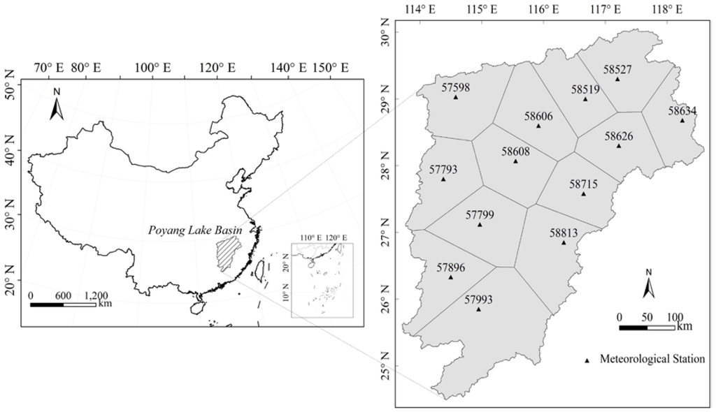
Figure 1.
Study area and location of the selected stations along with their Thiessen polygons.
The data sets of the study were acquired from the China Meteorological Data Sharing Service System (CMDSSS). Expect for the newly-built stations (after 2007) and stations with default data, this study selected 13 national meteorological stations. The monthly precipitation records for the period of 1957–2014 were available. The locations of the selected national meteorological stations are shown in Figure 1. In addition, the main characteristics of these stations are listed in Table S1.
3. Results
3.1. Areal Weights Obtained from the Thiessen Polygons Approach
The Thiessen polygons of 13 meteorological stations in the Poyang Lake Basin are shown in Figure 1. The weighting values of individual Thiessen polygons are listed in Table 2.
Table 2.
Weighting values of selected meteorological stations.
Table 2 shows that most weighting values ranged from 0.06 to 0.09. The largest weighting value was 0.16 for the Ganzhou meteorological station (code: 57993) located in the south of the Poyang Lake Basin, while the smallest weight value was 0.05 for the Yushan station (code: 58634) lied in the northeast of the basin. It indicated that the selected meteorological stations were relatively even as a whole. The values were used in computing areal mean precipitation and SPI.
3.2. Frequency Distribution of Site-Scale and Site-Averaged Precipitation
The Kolmogorov-Smirnov test demonstrated that the monthly precipitation followed Gamma distribution at all the selected meteorological stations for 1957–2014. So is the site-averaged precipitation sequence. Table 3 shows the shape parameter values of Gamma distribution. As indicated in Table 3, in terms of all the selected meteorological stations, the annual tendency of shape parameters for almost all stations at first increased and then decreased. The greater shape parameters ranged from 4.81 to 8.52 in April, whereas the less shape parameters ranged at 1.11–1.56 in November (or 1.15–1.61 in December). After processing by precipitation-average scheme, the shape parameter values of Gamma distribution for Case B were generally larger than that for individual stations, especially in March-September. In addition, the shape parameter values for Case B were greater than 8 in March (8.31), April (9.96), May (9.22), and June (10.53), but less than 5 in other months. It indicated that precipitation-density curves were closer to the normal distribution for Case B in March–June.
Table 3.
Shape parameters of Gamma distribution for 13 stations and that for precipitation-average scheme from January to December.
Figure 2 displays the cumulative-probability curves for 13 stations and Case B in January–December. The cumulative-probability curves were highlighted in red color for Case B. The distribution curves were more dispersed in February–September than other months. Moreover, the growth rate was generally faster for Case B, indicating more clustered precipitation for the period, which was consistent with that shown in Table 3. Noticeably, the cumulative probabilities at less precipitation for Case B were generally smaller than that for most of stations, but greater than that for most of stations at larger precipitation. The phenomenon was more distinctly observed in February–September (Figure 2). It indicated there was less frequency at relatively less or larger precipitation, while the majority of precipitation was located in the middle part of the gamma density distribution.
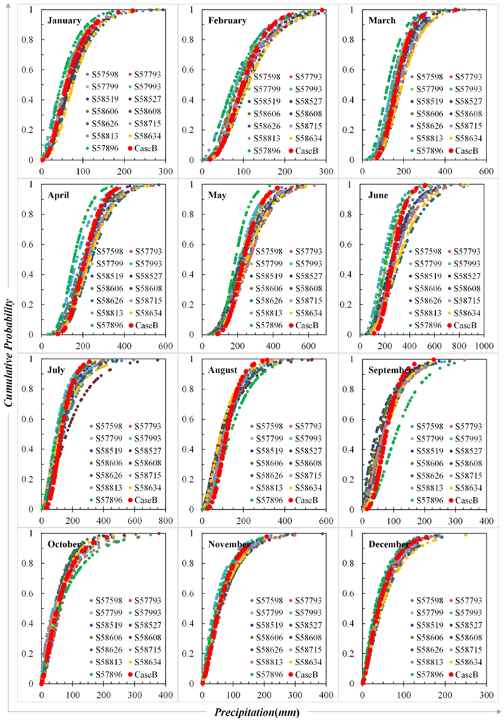
Figure 2.
The precipitation-cumulative probability curves of stations selected and the precipitation-average scheme in January–December.
3.3. Comparison of Case A and Case B for Drought Identification
Figure 3 illustrates the SPI time series obtained from two different processing schemes. The tendencies of the Poyang Lake Basin meteorological droughts were described by y = 5E-06x − 0.166 (R2 = 0.0018) for SPI time series obtained from Case A and y = 8E-06x − 0.252 (R2 = 0.0025) for SPI time series obtained from Case B, where x is the calendar month, respectively. Both series had similar features and trends of regional meteorological droughts. The slope of regression line was approximately 0 for either case. The fluctuation pattern generally stayed consistent, while their extreme values were greater for Case B than that for Case A. It implied that the Case A processing scheme could reduce the spatiotemporal variability in precipitation.
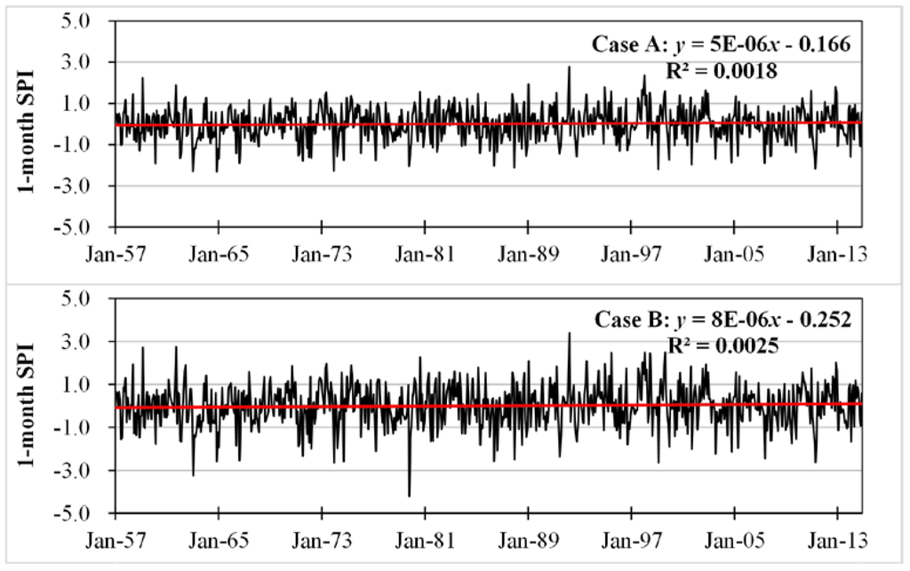
Figure 3.
SPI time series obtained from the SPI-mean scheme (Case A) and from the precipitation-mean scheme (Case B), along with fitted regression lines, for the Poyang Lake Basin in 1957–2014.
Table 4 shows the statistics of meteorological droughts obtained from two different processing schemes, in terms of drought event number, drought duration, and drought severity. The Case B processing schemes identified 162 drought events for 1957–2014, which was only one more than that for Case A. The drought duration ranged from 1 month to 11 months with 2.13 ± 1.72 months for Case A, approximately equal to that for Case B (2.13 ± 1.69 months). However, drought severity ranged at 0–12.26 with 1.70 ± 1.65 for Case B, generally greater than that for Case A. The quantitative statistical relationship of drought duration and severity of all drought events from two processing schemes was given in Figure 4. As indicated in Figure 4, the durations of most of drought events ranged from 1 to 4 months. The severity of drought events was generally aggravated in the case of Case B compared to that of Case A, which was also exhibited in Figure S1. Severe meteorological drought events were captured such as in 1963, 1978, 1997, 2003, and 2013 (Figure 4 and Figure S1). Moreover, the onset and termination time were almost identical for all the individual drought events. In addition, the slope of linear relationship for Case B was 0.7855 (R2 = 0.649), which was larger than 0.6146 (R2 = 0.6309) for Case A. In general terms, compared with that for Case B, the drought severity for Case A was generally smaller at the same drought duration. It might impact on drought assessment and quantitative approaches related to it.
Table 4.
Statistics of meteorological droughts obtained from two different processing schemes.
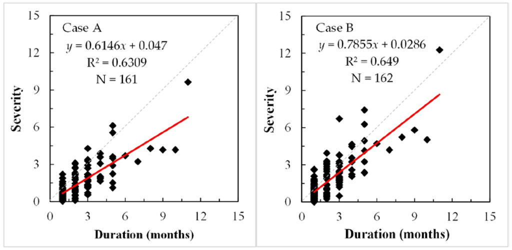
Figure 4.
Scatter plot with fitted regression line of drought duration and severity of drought events obtained from two different processing schemes for the Poyang Lake Basin in 1957–2014.
3.4. Difference in Drought Identification between Two Processing Schemes
Figure 5 shows change of probability of detection (POD) varying with available meteorological stations for regional drought monitoring. As indicated in Figure 5, POD increased gradually with more available stations in both processing schemes. When the available stations were less than 8 (61.5% of total stations), POD was obviously higher for Case B than Case A. When the station number was more than 8, POD approached to 91%–100% for both processing schemes. In this case, both schemes could identify the regional droughts with a high detectability.
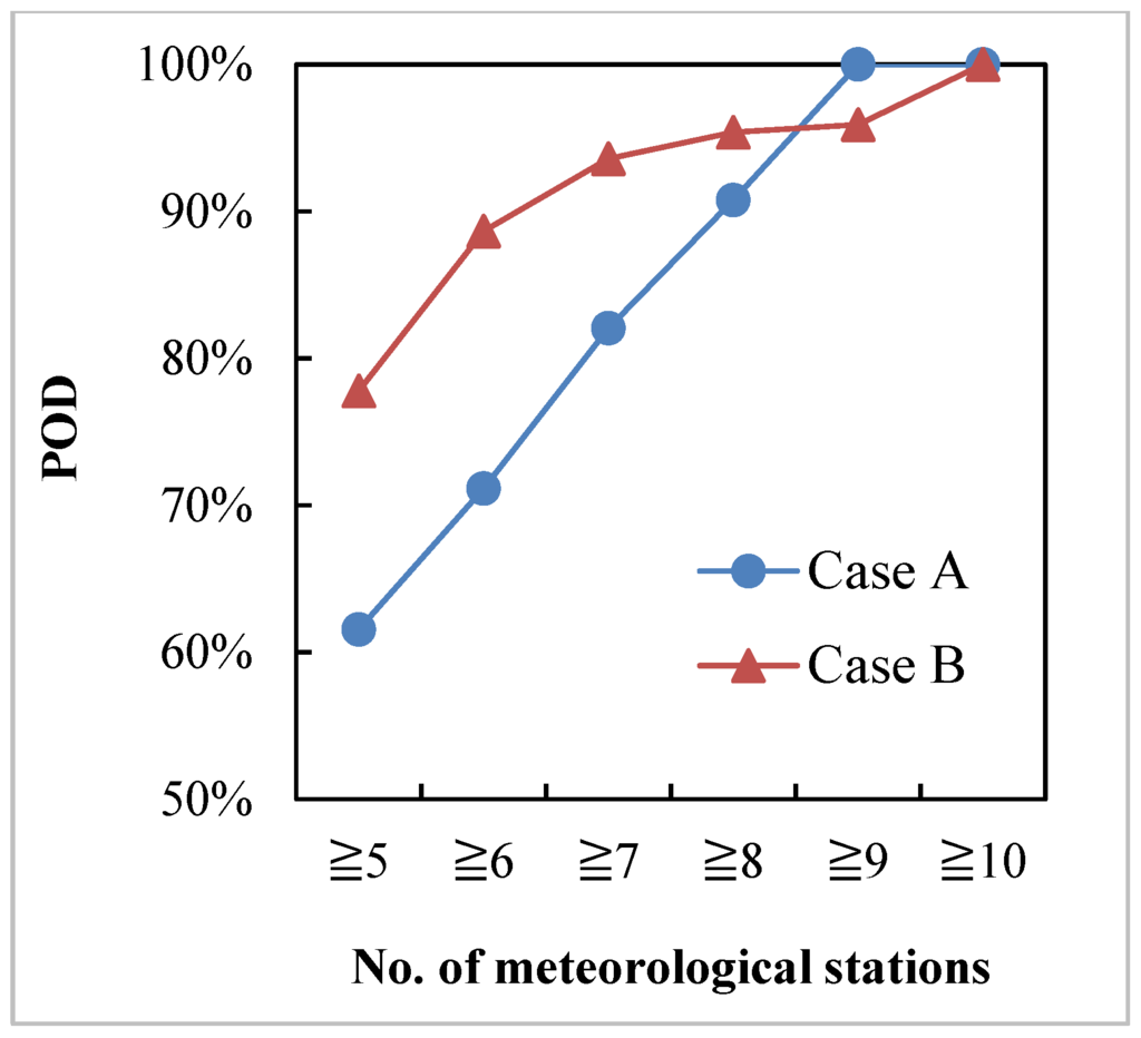
Figure 5.
The relationships between probability of detection (POD) and station numbers for monitoring regional meteorological droughts with two different processing schemes.
The difference of both processing schemes in drought detectability is related to available stations for monitoring. Figure 6 illustrates the relationship between ΔSPI and the number of meteorological stations for monitoring regional droughts. The statistics relationship of x (number of available meteorological stations) versus y (mean ΔSPI) was described by y = 0.0309x − 0.0026 (R2 = 0.773, p < 0.005). It indicated that ΔSPI had a positive correlation with the station number in the same period (p < 0.005). When the number of stations exceeded 10 (76.9% of total stations), ΔSPI was higher than 0.284. It reached up to 0.489 for 13 stations.
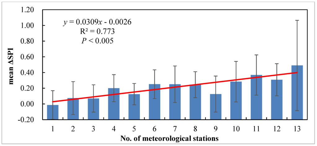
Figure 6.
The relationship between ΔSPI (= SPIA − SPIB) and the number of meteorological stations for monitoring regional droughts in the same period, along with a regression line for the relationship.
The relationship between ΔSPI and number of stations is also drought-level dependent. Table 5 shows that ΔSPI varied with number of stations for monitoring regional droughts of different levels. ΔSPI increased with the aggravated meteorological droughts. For example, in the case of ≥7 stations, ΔSPI was 0.305 ± 0.313 for moderate droughts and above, 0.412 ± 0.409 for severe droughts and above, and 0.616 ± 0.559 for extreme droughts. It suggested that the drought levels may have changed due to the difference in two processing schemes. Moreover, ΔSPI was enhanced with an increase of the number of stations. For example, when number of stations increased from 7 to 10, in the case of moderate droughts and above, the ΔSPI mean increased from 0.305 to 0.368. Moreover, the ΔSPI mean changed from 0.616 to 0.759 for Extreme droughts. Therefore, different processing schemes may result in significant impacts on regional drought assessment.
Table 5.
The difference between two processing schemes (ΔSPI) for monitoring regional droughts of different levels varying with number of stations.
Furthermore, the relationship between ΔSPI and number of stations had seasonal variation. Figure 7 shows the variation under three different situations. The multi-year mean ΔSPI at first increased and then decreased. The maximum variation (ΔSPI = 0.662 for ≥7 stations) was in June, whereas the minimum (ΔSPI = 0.139 for ≥7 stations) appeared in November. When the number of stations was ≥9, the multi-year mean ΔSPI reached up to 0.916 in June and down to 0.151 in November. The phenomenon was found in other calendar month with ≥10 stations. Hence, ΔSPI aggravated gradually with an increase of number of stations for monitoring regional droughts in the same period, even if the annual tendency remained unchanged.
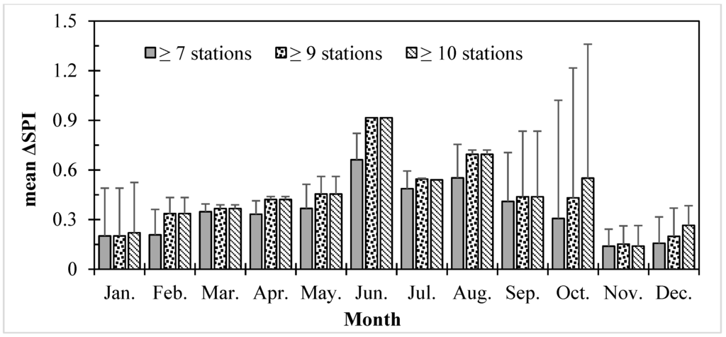
Figure 7.
Seasonal variation of ΔSPI and its change with station number for monitoring regional droughts in the same period.
Change in ΔSPI can be explained through inter-comparison between monthly SPI values of two processing schemes. Table 6 displays the statistical indicators of linear relationship of the SPI values of two schemes for each calendar month. The SPI series had a significantly positive correlation between Case A and Case B for every month (R2 > 0.93). The intercept of linear regression relationship was approximately 0 for each calendar month. The slopes of the linear regression increased from January and then decreased after June. The maximum slope was 1.5625 in June, but the minimum slope was 1.0925 in December. Meanwhile, the slope values were larger than 1.2 in March–September. It was in January and December that the slope values were approximately equal to 1. The greater slope values appeared in March-September, which indicated that the larger difference between two different processing schemes could occur in these months as well, as shown in Figure 7. The phenomena confirmed that the SPI series from either processing schemes depicted the annual tendency of the basin-scale droughts.
Table 6.
The linear relationship of SPI series from two processing schemes (independent variable: SPI series obtained from precipitation-mean scheme, dependent variable: SPI series captured from SPI-mean scheme).
Notably, some points deviated away from their sequences in different degrees, namely, in January and October (Table 6). For example, the SPI value for Case B in October 1979 was as low as −4.20, whereas the SPI value for Case A was −2.04. In terms of 13 selected meteorological stations, the SPI values of 2 stations (15.4% of total stations) were −1.74 and −1.82 (belongs to −2.0 ~ −1.5), which represented the severe meteorological droughts. The SPI values of 11 stations (84.6% of total stations) were smaller than −2.0, which indicated the extreme meteorological droughts. Moreover, the cumulative probabilities of 13 meteorological stations ranged from 0.015 to 0.05. However, the cumulative probability for Case B was 1.3E-05 in the period, which was approximately equal to zero. Hence, when cumulative probability was transformed into SPI by the inverse of cumulative standard normal function, the SPI value for Case B was far less than that for Case A. the phenomena confirmed that the precipitation-mean processing scheme (Case B) could make the less precipitation recorded by most or all of stations deviated from the precipitation-mean series more seriously.
Figure 8a shows three precipitation-density curves. Curve I and Curve II exhibited positive skew-distribution, whereas the curve for Case B was close to normal distribution. The maximum precipitation frequency peak was found in Case B obtained from the precipitation-mean scheme. Therefore, the precipitation-mean processing scheme generally weakens the extreme precipitation and made the precipitation series smoother. Then, when the precipitation was P, the cumulative probabilities from largest to smallest were in Curve I, Curve II, and Case B (Figure 8b). Furthermore, when the precipitation was less than P, the cumulative probability for Case B was even much smaller. Finally, the cumulative probabilities for three curves at P value were transformed into SPII, SPIII, and SPIB through the inverse of the cumulative standard normal distribution function respectively (Figure 8c). The mean of SPII and SPIII was distinctly larger than SPIB.
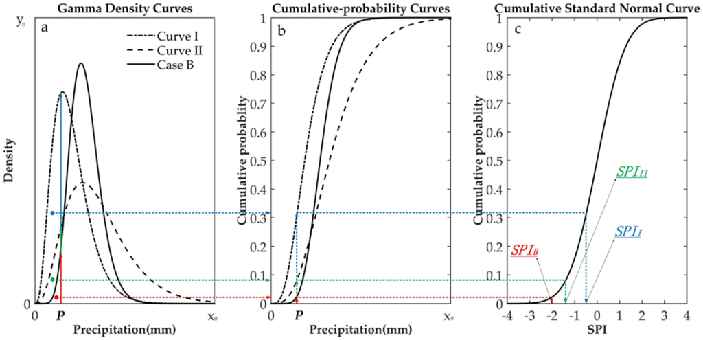
Figure 8.
Explanation of transformation from precipitation density (a) to precipitation cumulative probability (b) to SPI (c), Curve I and Curve II represents the corresponding gamma density curves of a station with minimum mean precipitation and a station with maximum mean precipitation, respectively.
In essence, when the P represented dry condition (i.e., less precipitation), the frequency of less precipitation in their individual long-term precipitation series observed by meteorological station was higher relatively (e.g., in Curve I and Curve II). Moreover, the varying gradients of precipitation were also more even and more stationary relatively. However, when the less precipitation happened to record by most or all of selected meteorological stations at the same period, the precipitation density at P for Case B processed by the precipitation-mean processing scheme was much smaller (e.g., in curve for Case B). That is to say, the less precipitation in the period for Case B would deviated away from the precipitation-mean series more seriously, as indicated in Figure 8a,b. In this case, then, the precipitation density integration at P was transformed into the cumulative probability by the gamma cumulative distribution function. The cumulative probability at P for Case B was much smaller than that for the other curves (Figure 8b). Finally, when the less precipitation was transformed to SPI value, the extreme SPI value would be calculated. Moreover, the smaller the precipitation was, the less the SPI value was. This was why the some points deviated from the SPI series in Table 6 such as in January, June, and October.
4. Discussion
This study investigated the effects of two different processing schemes on meteorological drought assessment with long-term precipitation data in the Poyang Lake Basin for 1957–2014. The results provide the important evidences on selection of a suitable scheme for reliable assessment of regional droughts.
In a view of drought identification, both processing schemes revealed the similar long-term trend, number of drought events, and drought duration as well. Hence, the two schemes were often used to analyze the characteristics and tendency of regional drought [31,56]. However, the drought severity was generally alleviated in the case of the SPI-mean scheme compared to that of the precipitation-mean scheme. In the study of Dash et al. [41], we noticed that the SPI series from selected individual stations had barely extreme SPI values (SPI > 3.0 or SPI < −3.0), whereas the extreme values (even SPI > 4.0 or SPI < −4.0) were found frequently in SPI series obtained from the regional average of observed data in the research. The details exhibited by Dash et al. are consistent with the results of the research. Additionally, the relationship between drought characteristics, especially drought duration and drought severity, is often used for constructing drought probabilistic models [42,56]. However, due to the difference in drought duration and severity obtained from two processing schemes (Figure 4), it might affect the drought quantitative approaches related to them.
From a perspective of regional drought monitoring, ΔSPI between two SPI series had a significantly positive correlation with the number of stations (p < 0.005). The number of stations recording less precipitation at the same period could be applied to represent the severity of dry condition (i.e., precipitation deficit). Therefore, the more the number of stations (i.e., precipitation deficit) were, the larger the difference obtained from two processing schemes was (Table 5). When one drought occurs over the region, the quantitative assessment should be taken seriously. In addition, the study is relevant in satellite remote sensing of precipitation and its application to monitor regional drought [57]. Satellite precipitation data generally cover large areas (e.g., 25 km for TRMM). In essence, these data can be considered as spatially averaged. Use of these data may generate different results from those of ground observations. Therefore, the research can provide implications for accurate drought monitoring using satellite precipitation data.
A quantified comparison with two SPI series was carried out addressing a significantly positive correlation between Case A and Case B for every month. The annual tends of the slope values of the linear regression at first increased from January and then decreased after June. The slope values were larger than 1.20 in March-September, suggesting the greater difference between precipitation-mean scheme and SPI-mean scheme. From a perspective of the transformation from precipitation density to cumulative probability to SPI calculation, the study revealed the causes of the difference between two processing schemes. The precipitation-mean processing scheme averaged and weakened the extreme precipitation situations and made the precipitation more clustered in some certain (Table 3 and Figure 2). However, when less precipitation was recorded by most or all of the meteorological stations over the basin, less precipitation would be deviated from the new precipitation-mean series more seriously (Figure 8). Smaller density was found in the precipitation-density curve. Comparison with the cumulative probabilities for other meteorological stations at the less precipitation, the cumulative probability for Case B was less. Therefore, the less SPI value was calculated through the inverse of cumulative standard normal distribution function (Figure 8). Based on calculation principles, the mean-precipitation processing scheme is first linear and then nonlinear transformation, and the mean-SPI scheme just the opposite. It is just in the homogeneous areas that the two processing schemes may produce the same results.
5. Conclusions
Compared with the performances in assessing the regional meteorological drought from two different processing schemes, the following conclusions may be made:
- (1)
- Both processing schemes could express the similar monitoring trends, number of drought events, and drought duration as well. However, the drought severity in the case of the precipitation-mean scheme was generally smaller than that of the SPI-mean scheme.
- (2)
- The difference from two processing schemes had a significantly positive correlation with the number of stations monitoring drought (p < 0.005). Moreover, sometimes, the difference was so large that it could change meteorological drought levels.
- (3)
- The precipitation-mean scheme reduced the extent of precipitation deficits and made the precipitation more clustered in some certain. Meanwhile, it made less precipitation deviate from the precipitation-mean series farther when the less precipitation has wide spatial distribution over the region. However, the SPI-mean scheme can accurately highlight the relatively serious and universal dry situations occurred over the region. Therefore, on regional meteorological drought monitored effectively basis, for representing regional meteorological drought reliably, the SPI-mean scheme is more likely to satisfy the physical.
Supplementary Materials
The following are available online at www.mdpi.com/2073-4441/8/9/373/s1, Table S1: Characteristics of the meteorological station, Figure S1: Time series of drought severity obtained with two different processing schemes for the Poyang Lake Basin in 1957–2014.
Acknowledgments
This work was supported by the State Key Program of National Natural Science of China under Grant 41430855.
Author Contributions
Han Zhou performed the study, collected and analyzed the data, and wrote the manuscript. Yuanbo Liu proposed the main idea, designed the study and revised the manuscript.
Conflicts of Interest
The authors declare no conflict of interest.
References
- Rossi, G.; Benedini, M.; Tsakiris, G.; Giakoumakis, S. On regional drought estimation and analysis. Water Resour. Manag. 1992, 6, 249–277. [Google Scholar] [CrossRef]
- Obasi, G.O.P. Wmo’s role in the international decade for natural disaster reduction. Bull. Am. Meteorol. Soc. 1994, 75, 1655–1661. [Google Scholar] [CrossRef]
- Spinoni, J.; Naumann, G.; Carrao, H.; Barbosa, P.; Vogt, J. World drought frequency, duration, and severity for 1951–2010. Int. J. Climatol. 2014, 34, 2792–2804. [Google Scholar] [CrossRef]
- Mishra, A.K.; Singh, V.P. A review of drought concepts. J. Hydrol. 2010, 391, 202–216. [Google Scholar] [CrossRef]
- Mpelasoka, F.; Hennessy, K.; Jones, R.; Bates, B. Comparison of suitable drought indices for climate change impacts assessment over australia towards resource management. Int. J. Climatol. 2008, 28, 1283–1292. [Google Scholar] [CrossRef]
- Kallis, G. Droughts. Annu. Rev. Environ. Resour. 2008, 33, 85–118. [Google Scholar] [CrossRef]
- Gumbel, E.J. Statistical forecast of droughts. Int. Assoc. Sci. Hydrol. Bull. 1963, 8, 5–23. [Google Scholar] [CrossRef]
- Palmer, W.C. Meteorological Drought; US Department of Commerce, Weather Bureau: Washington, DC, USA, 1965.
- Dracup, J.A.; Lee, K.S.; Paulson, E.G., Jr. On the definition of droughts. Water Resour. Res. 1980, 16, 297–302. [Google Scholar] [CrossRef]
- Wilhite, D.; Glantz, M. Understanding: The drought phenomenon: The role of definitions. Water Int. 1985, 10, 111–120. [Google Scholar] [CrossRef]
- Stanley, A.; Changnon, J.; Easterllng, W.E. Measuring drought impacts the illinois case. Water Resour. Bull. 1989, 25, 27–42. [Google Scholar]
- Hao, Z.C.; Singh, V.P. Drought characterization from a multivariate perspective: A review. J. Hydrol. 2015, 527, 668–678. [Google Scholar] [CrossRef]
- Society, A.M. Policy statement: Meteorological drought. Bull. Am. Meteorol. Soc. 1997, 78, 847–849. [Google Scholar]
- Peters, E. Propagation of Drought through Groundwater Systems: Illustrated in the Pang (UK) and Upper-guadiana (es) Catchments. Ph.D. Thesis, Wageningen University, Wageningen, The Netherlands, 2003. [Google Scholar]
- Zargar, A.; Sadiq, R.; Naser, B.; Khan, F.I. A review of drought indices. Environ. Rev. 2011, 19, 333–349. [Google Scholar] [CrossRef]
- Eltahir, E.A.B.; Yeh, P.J.F. On the asymmetric response of aquifer water level to floods and droughts in illinois. Water Resour. Res. 1999, 35, 1199–1217. [Google Scholar] [CrossRef]
- Peters, E.; Torfs, P.J.J.F.; van Lanen, H.A.J.; Bier, G. Propagation of drought through groundwater—A new approach using linear reservoir theory. Hydrol. Process. 2003, 17, 3023–3040. [Google Scholar] [CrossRef]
- Van Loon, A.F.; van Lanen, H.A.J.; Tallaksen, L.M.; Hanel, M.; Fendeková, M.; Machlica, A.; Sapriza, G.; Koutroulis, A.; van Huijgevoort, M.H.J.; Jódar Bermúdez, J.; et al. Propagation of Drought through the Hydrological Cycle; WATCH Technical Report 31; Wageningen University: Wageningen, The Netherlands, 2011. [Google Scholar]
- Potop, V. Evolution of drought severity and its impact on corn in the republic of moldova. Theor. Appl. Climatol. 2011, 105, 469–483. [Google Scholar] [CrossRef]
- Al-Faraj, F.A.M.; Scholz, M.; Tigkas, D.; Boni, M. Drought indices supporting drought management in transboundary watersheds subject to climate alterations. Water Policy 2015, 17, 865–886. [Google Scholar] [CrossRef]
- Akhtari, R.; Morid, S.; Mahdian, M.H.; Smakhtin, V. Assessment of areal interpolation methods for spatial analysis of spi and edi drought indices. Int. J. Climatol. 2009, 29, 135–145. [Google Scholar] [CrossRef]
- Zhang, Q.; Sun, P.; Li, J.; Xiao, M.; Singh, V.P. Assessment of drought vulnerability of the Tarim River basin, Xinjiang, China. Theor. Appl. Climatol. 2014, 121, 337–347. [Google Scholar] [CrossRef]
- Pei, W.; Fu, Q.; Liu, D.; Li, T.-X.; Cheng, K. Assessing agricultural drought vulnerability in the Sanjiang plain based on an improved projection pursuit model. Nat. Hazards 2016, 82, 683–701. [Google Scholar] [CrossRef]
- Tallaksen, L.M.; Hisdal, H.; Lanen, H.A.J.V. Space-time modelling of catchment scale drought characteristics. J. Hydrol. 2009, 375, 363–372. [Google Scholar] [CrossRef]
- Vrochidou, A.E.K.; Tsanis, I.K.; Grillakis, M.G.; Koutroulis, A.G. The impact of climate change on hydrometeorological droughts at a basin scale. J. Hydrol. 2013, 476, 290–301. [Google Scholar] [CrossRef]
- McKee, T.B.; Doesken, N.J.; Kleist, J. The relationship of drought frequency and duration to time scales. In Proceedings of the 8th Conference on Applied Climatology; American Meteorological Society: Boston, MA, USA, 1993; Volume 17, pp. 179–183. [Google Scholar]
- Byun, H.-R.; Wilhite, D.A. Objective quantification of drought severity and duration. J. Clim. 1999, 12, 2747–2756. [Google Scholar] [CrossRef]
- Tsakiris, G.; Vangelis, H. Establishing a drought index incorporating evapotranspiration. Eur. Water 2005, 9, 3–11. [Google Scholar]
- Vicente-Serrano, S.M.; Beguería, S.; López-Moreno, J.I. A multiscalar drought index sensitive to global warming: The standardized precipitation evapotranspiration index. J. Clim. 2010, 23, 1696–1718. [Google Scholar] [CrossRef]
- Hayes, M.J.; Svoboda, M.D.; Wilhite, D.A.; Vanyarkho, O.V. Monitoring the 1996 drought using the standardized precipitation index. Bull. Am. Meteorol. Soc. 1999, 80, 429–438. [Google Scholar] [CrossRef]
- Livada, I.; Assimakopoulos, V.D. Spatial and temporal analysis of drought in greece using the standardized precipitation index (SPI). Theor. Appl. Climatol. 2007, 89, 143–153. [Google Scholar] [CrossRef]
- Shiau, J.T.; Modarres, R. Copula-based drought severity-duration-frequency analysis in iran. Meteorol. Appl. 2009, 16, 481–489. [Google Scholar] [CrossRef]
- Qian, B.; Zhang, X.; Chen, K.; Feng, Y.; O’Brien, T. Observed long-term trends for agroclimatic conditions in Canada. J. Appl. Meteorol. Climatol. 2010, 49, 604–618. [Google Scholar] [CrossRef]
- Bonsal, B.R.; Aider, R.; Gachon, P.; Lapp, S. An assessment of canadian prairie drought: Past, present, and future. Clim. Dyn. 2013, 41, 501–516. [Google Scholar] [CrossRef]
- Jenkins, K.; Warren, R. Quantifying the impact of climate change on drought regimes using the standardised precipitation index. Theor. Appl. Climatol. 2015, 120, 41–54. [Google Scholar] [CrossRef]
- Merino, A.; López, L.; Hermida, L.; Sánchez, J.L.; García-Ortega, E.; Gascón, E.; Fernández-González, S. Identification of drought phases in a 110-year record from western mediterranean basin: Trends, anomalies and periodicity analysis for iberian peninsula. Glob. Planet. Chang. 2015, 133, 96–108. [Google Scholar] [CrossRef]
- Svoboda, M.D.; Fuchs, B.A.; Poulsen, C.C.; Nothwehr, J.R. The drought risk atlas: Enhancing decision support for drought risk management in the United States. J. Hydrol. 2015, 526, 274–286. [Google Scholar] [CrossRef]
- Hayes, M.; Svoboda, M.; Wall, N.; Widhalm, M. The lincoln declaration on drought indices: Universal meteorological drought index recommended. Bull. Am. Meteorol. Soc. 2011, 92, 485–488. [Google Scholar] [CrossRef]
- Zhai, J.; Su, B.; Krysanova, V.; Vetter, T.; Gao, C.; Jiang, T. Spatial variation and trends in PDSI and SPI indices and their relation to streamflow in 10 large regions of China. J. Clim. 2010, 23, 649–663. [Google Scholar] [CrossRef]
- Gao, L.; Zhang, Y. Spatio-temporal variation of hydrological drought under climate change during the period 1960–2013 in the Hexi Corridor, China. J. Arid Land 2016, 8, 157–171. [Google Scholar] [CrossRef]
- Dash, B.K.; Rafiuddin, M.; Khanam, F.; Islam, M.N. Characteristics of meteorological drought in Bangladesh. Nat. Hazards 2012, 64, 1461–1474. [Google Scholar] [CrossRef]
- Mishra, A.K.; Singh, V.P.; Desai, V.R. Drought characterization: A probabilistic approach. Stoch. Environ. Res. Risk Assess. 2007, 23, 41–55. [Google Scholar] [CrossRef]
- Vicente-Serrano, S.M. Differences in spatial patterns of drought on different time scales: An analysis of the iberian peninsula. Water Resour. Manag. 2006, 20, 37–60. [Google Scholar] [CrossRef]
- The Ramsar Convention. The List of Wetlands of International Importance. Available online: http://www.ramsar.org/document/the-list-of-wetlands-of-international-importance-the-ramsar-list (accessed on 3 May 2016).
- Liu, Y.; Wu, G. Hydroclimatological influences on recently increased droughts in China’s largest freshwater lake. Hydrol. Earth Syst. Sci. 2016, 20, 93–107. [Google Scholar] [CrossRef]
- Liu, Y.B.; Wu, G.; Guo, R.F.; Wang, R.G. Changing landscapes by damming: The three gorges dam causes downstream lake shrinkage and severe droughts. Landsc. Ecol. 2016. [Google Scholar] [CrossRef]
- Thom, H.C.S. A note on the gamma distribution. Mon. Weather Rev. 1958, 86, 117–122. [Google Scholar] [CrossRef]
- Milton, A.; Stegun, I.A. Handbook of Mathematical Functions: With Formulas, Graphs, and Mathematical Tables; Courier Corporation: New York, NY, USA, 1965. [Google Scholar]
- Johnson, D.; Smith, M.; Koren, V.; Finnerty, B. Comparing mean areal precipitation estimates from nexrad and rain gauge networks. J. Hydrol. Eng. 1999, 4, 117–124. [Google Scholar] [CrossRef]
- Fiedler, F. Simple, practical method for determining station weights using thiessen polygons and isohyetal maps. J. Hydrol. Eng. 2003, 8, 219–221. [Google Scholar] [CrossRef]
- Squires, G.L. Practical Physics; Cambridge University Press: Cambridge, UK, 2001. [Google Scholar]
- Gosset, M.; Viarre, J.; Quantin, G.; Alcoba, M. Evaluation of several rainfall products used for hydrological applications over west africa using two high-resolution gauge networks. Q. J. R. Meteorol. Soc. 2013, 139, 923–940. [Google Scholar] [CrossRef]
- Hu, Q.; Feng, S.; Guo, H.; Chen, G.; Jiang, T. Interactions of the yangtze river flow and hydrologic processes of the Poyang Lake, China. J. Hydrol. 2007, 347, 90–100. [Google Scholar] [CrossRef]
- Canadell, J.G.; Steffen, W.L.; White, P.S. Igbp_gcte terrestrial transects dynamics ofterrestrial ecosystems under environmental change. J. Veg. Sci. 2002, 13, 297–450. [Google Scholar]
- Liu, Y.; Wu, G.; Zhao, X. Recent declines in China’s largest freshwater lake: Trend or regime shift? Environ. Res. Lett. 2013, 8, 014010. [Google Scholar] [CrossRef]
- Janga Reddy, M.; Ganguli, P. Application of copulas for derivation of drought severity-duration-frequency curves. Hydrol. Process. 2012, 26, 1672–1685. [Google Scholar] [CrossRef]
- Tao, H.; Fischer, T.; Zeng, Y.; Fraedrich, K. Evaluation of TRMM 3B43 precipitation data for drought monitoring in Jiangsu Province, China. Water 2016, 8, 221. [Google Scholar] [CrossRef]
© 2016 by the authors; licensee MDPI, Basel, Switzerland. This article is an open access article distributed under the terms and conditions of the Creative Commons Attribution (CC-BY) license (http://creativecommons.org/licenses/by/4.0/).