1. Introduction
Reservoirs, as projects to regulate runoff, play an important role in making water resources more suitable for social development and environmental protection. Making reasonable regulation rules is significant for reservoirs to play roles in water resources allocation [
1,
2,
3,
4]. Based on the research of reservoir release, starting standard, ending condition, and the determination of periods supplying water, different kinds of water supply rules have been put forward, such as Pack Rule (PR) [
5], Space Rule (SP) [
6], New York City Rule (NYC) [
7], Linear Decision Rule (LDR) [
8] and Standard Operation Policy (SOP) [
5], Hedging Rules (HR) [
9,
10,
11,
12,
13], and so on. Among the rules, the SOP is widely applied in reservoir operation. The maximum water supply and minimum water shortage of the water supply system are chosen by SOP [
10]. The reservoir water is fully released under SOP when the available water is smaller than the water demand. During the dry season, water is not reserved in advance under SOP, which will cause severe damage for water supply in the later period. HR is obtained on the basis of optimizing the operation rules of SOP in dry season, which is an effective measure for reservoir regulation [
14]. In order to avoid severe water deficit of a few periods in the dry season, HR mostly chooses several periods to decrease the water supply so that water can be reserved for the later period [
15]. The loss caused by a severe water deficit of a few periods is more serious than that caused by the slight water shortage of many periods.
HR determines the starting water availability according to the judgements of reservoir storage or available water in facing period [
10]. Bayazit
et al. [
16] proposed the starting water availability and ending water availability of hedging rules based on the judging condition of available water at the beginning or end of the period, and analyzed the influence of the available water threshold on reservoir release performance. Srinivasan
et al. [
17] added a hedging factor (HF) index on the basis of the available water threshold index at the beginning or end of the period by Bayazit
et al. [
16], and analyzed the influence of the three indices on reliability, resiliency, and vulnerability of reservoir release.
Currently, in the studies of hedging rules, the research of the two-period model is a hot issue. The two-period model divides operation periods into a facing period and remaining period. This study focuses on the operation rules through analyzing the water supply of a facing period and water storage target of the next period. The operation rules contact the water supply of the facing period, starting water availability (SWA), and ending water availability (EWA). The study mainly focuses on two aspects: one is the determination of the three elements of hedging rules, including the starting water availability (SWA), ending water availability (EWA), and hedging factors (HF); another is the influence of inflow uncertainty on operation rules [
18]. Draper
et al. [
10] and Shiau [
15] determined starting water availability according to marginal costs of reservoir storage and marginal benefits of reservoir release based on the marginal benefit principle of economics. According to different reservoir hedging thresholds, SWA and EWA are given by the analytical expression of the period water supply. You
et al. [
12] and Zhao
et al. [
19,
20] discussed effects of inflow uncertainty and reservoir operation constraint conditions on optimal conditions and operation rules of the two-period reservoir operation model.
In the two-period model, the weighting factor and water storage target are important parameters for determining hedging rules. Due to short-term defects of the two-period model, it is difficult to determine the weighting factor and water storage target. The two-period model chose the upper-basic operation curve as the storage target which could not guarantee the optimal release benefits in the long term. Therefore, this study proposes a hedging model that consists of the two-period model and parameter simulation and an optimization model. The relationship between the different operation periods is established by the optimization model of weighting factors and the release target, so it makes up the deficiency of the two-period model. This paper proposes a hedging rule which is composed of the two-period model and the parameter simulation optimization model. The two-period model is adopted for simulating the process of the water supply. The parameter simulation optimization model, with a particle swarm optimization algorithm, is adopted for optimizing the parameter. Heiquan reservoir is employed as a case study to verify the reasonability and efficiency of the hedging rule.
2. Methodology
2.1. Hedging Rules Based on the Two-Period Model
2.1.1. The Optimal Reservoir Release
For a water supply reservoir, the water availability at time
t is the sum of initial water stored in a reservoir at time
t plus the current inflow and minus the evaporation loss at this time period,
i.e.,
where
WAt, is the water availability of the reservoir during time period
t;
St,
It, and
Et are, respectively, the initial water stored in a reservoir at the beginning of time period
t, inflow into reservoir at time
t, evaporation and seepage loss at time
t.
By applying the principle of water balance, the initial water stored in a reservoir at the beginning of time period
t+1 is equal to the sum of the initial water stored in a reservoir at time
t plus the current inflow and minus the sum of evaporation loss and reservoir release at time period
t. That is:
where
Rt is the reservoir release at time
t, which is used for projected demand
Dt and constrained by 0
Rt Dt when considering breakage depth.
Equations (1) and (2) simplify to Equation (3):
Equation (3) implies that water availability during time period
t includes the reservoir release of the current period
Rt, along with water storage capacity
St+1 at the beginning time
t+1. The benefits of a water supply reservoir during a period can be separated into two parts, including the benefit of release and benefit of storage. The benefit of release is measured by water deficit loss at time
t, while the benefit of storage is measured by the difference between storage at the beginning of the next period and storage targets. The optimization framework of reservoir operation is to minimize the sum of the water supply benefit function
B(Rt) and the carryover storage benefit function
C(St+1) [
19].
B(Rt) and
C(St+1) is formulated as Equations (5) and (6):
where ω is the weighting factor assigned to the loss function of reservoir release target, m is an exponent to define the shape of the loss functions (m should exceed 1 in order to have a convex function that can be minimized).
The key finding of Draper and Lund [
10] was the derivation of the optimal hedging condition for a water supply reservoir, which states that the marginal benefit of release is equal to the marginal benefit of storage. That is:
Using the Equations (5)–(7), the optimal reservoir release
can be deduced, which is formulated as Equation (8):
2.1.2. Starting Water Availability (SWA) and Ending Water Availability (EWA) of Hedging Rules
A factor
, which is called the inverse-weighted target ratio (IWTR), is developed by Shiau [
19]. IWTR is defined as:
By putting Equation (9) into Equation (8), the optimal reservoir release
can be simplified using
, which is formulated as Equation (10):
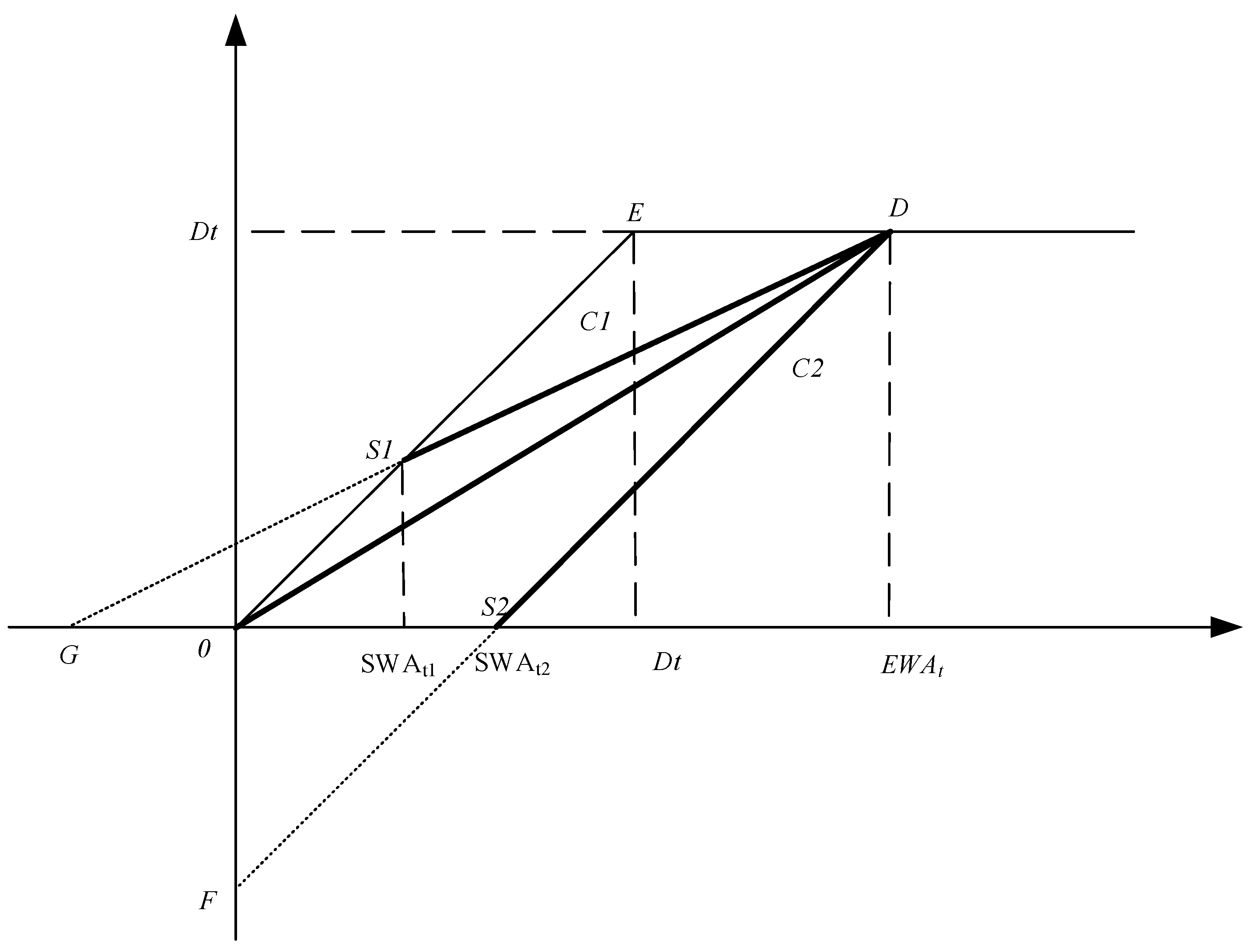
Under the hedging rules, when
m = 2, the relationship between the optimal reservoir release and water availability (WA) has a linear relationship with a slope of
. As demonstrated in
Figure 1, O-S1-D, O-D, and O-S2-D represent hedging rules under three different situations, where S1 and S2 are SWA and D is the EWA. In the figure, D is a fixed point, because
.
The linear optimal hedging of
is line OD, the slope of line OD is
. When
, Equation (10) can be simplified as:
It is shown from Equation (11) that WA is allocated according to the ratio of demand target and storage target, and the two targets get the same satisfaction degree in line OD. Line OD separates area O-S1-D-S2-O into two parts. As D is a fixed point, the slope of any line DS1 in the upper area of line OD is smaller than the slope of line OD. The slope of line DS1 is , so , then . As a result, when WA remains constant, is larger, and the satisfaction degree of the demand target is larger than that of the storage target. On the other hand, the slope of any line DS2 in the lower area of line OD is larger than the slope of line OD. The slope of line OS2 is , so , then . As a result, when WA remains constant, is smaller, and the satisfaction degree of the demand target is smaller than that of the storage target.
2.1.3. The Expression Form of Hedging Rules
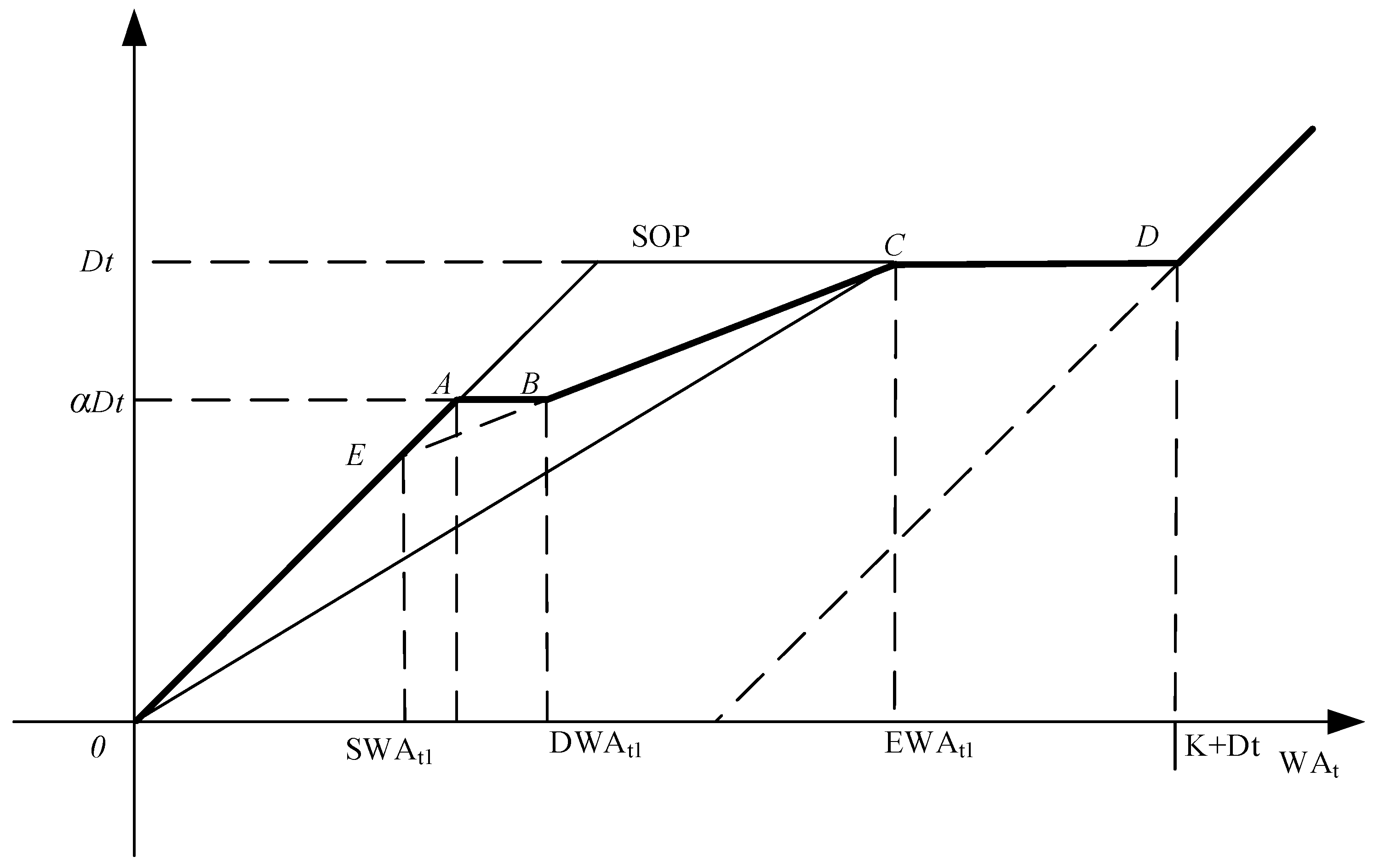
Damage depth is an important index for the ability of water supply of reservoir. This index for evaluating the reservoir with low inflow in dry season is particularly important. The acceptable damage depth (ADD) is used to express the vulnerability of water supply reservoir, generally defined as the proportion of the minimum water supply to the water demand in a single period for water-supply area. The minimum water supply is obtained by the minimum demand in different departments. The supply water is less than the minimum water supply, which can bring a devastating effect on the local economy. After considering ADD, hedging rules can be expressed in three situations, which is shown in
Table 1.
Situation I: Point E is defined as SWA by the traditional model. Point A of ADD is higher than Point E (
Figure 2). Water is supplied under the guide of the SOP rule in line EA. Point A is chosen as the SWA point, then the quantity of the water supply is kept fixed at an allowable damage depth in line AB, and point C is defined as the EWA point. In hedging rules:
,
,
.
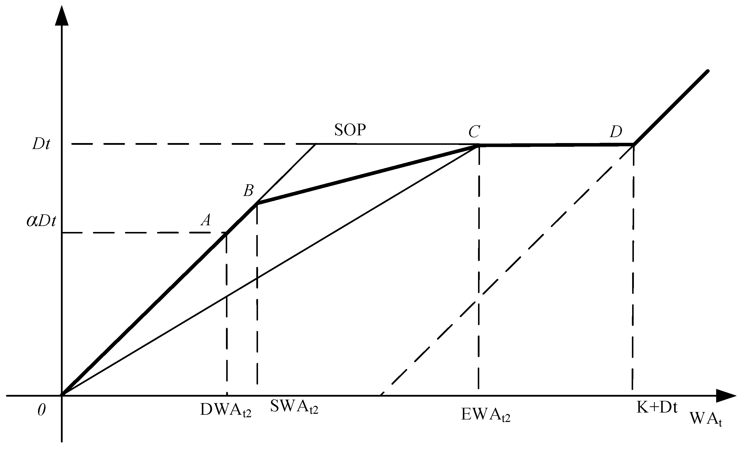
Situation II: Point B is defined as the SWA by the traditional model. Point A of ADD is lower than Point B (
Figure 3). Point B is chosen as the starting point and point C is chosen as the water-supply hedging ending point. In hedging rules:
,
,
.
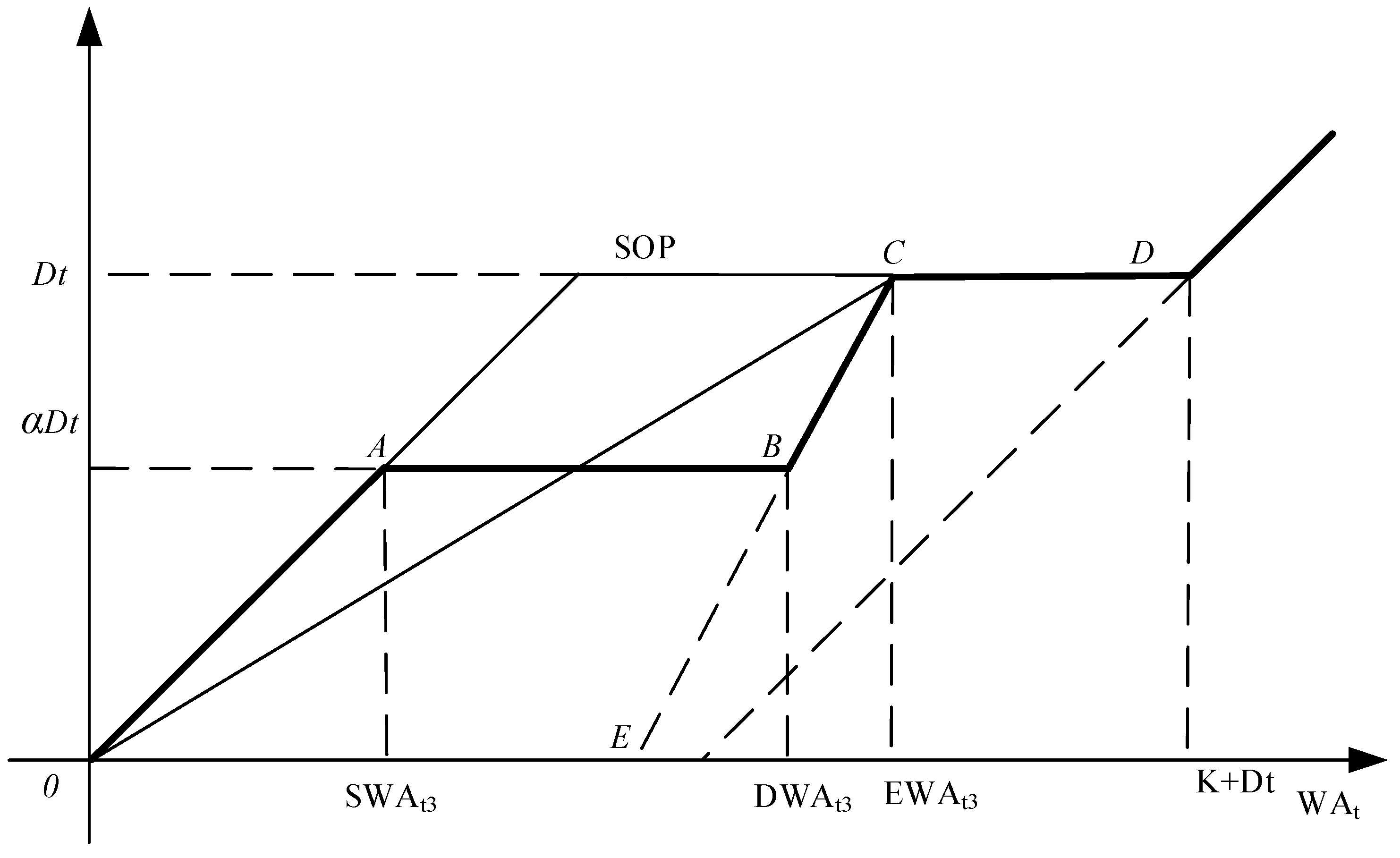
Situation III: Point A of ADD is higher than the water-supply hedging starting point E, which is defined as the SWA by the traditional model (
Figure 4). Point A is chosen as the starting point and point C is chosen as the water-supply hedging ending point, water is supplied under the guide of the SOP rule in line OA and the quantity of water supply is kept fixed at an allowable damage depth in line AB. In hedging rules:
,
,
.
2.2. Parameter Simulation and Optimization Model in Hedging Rules
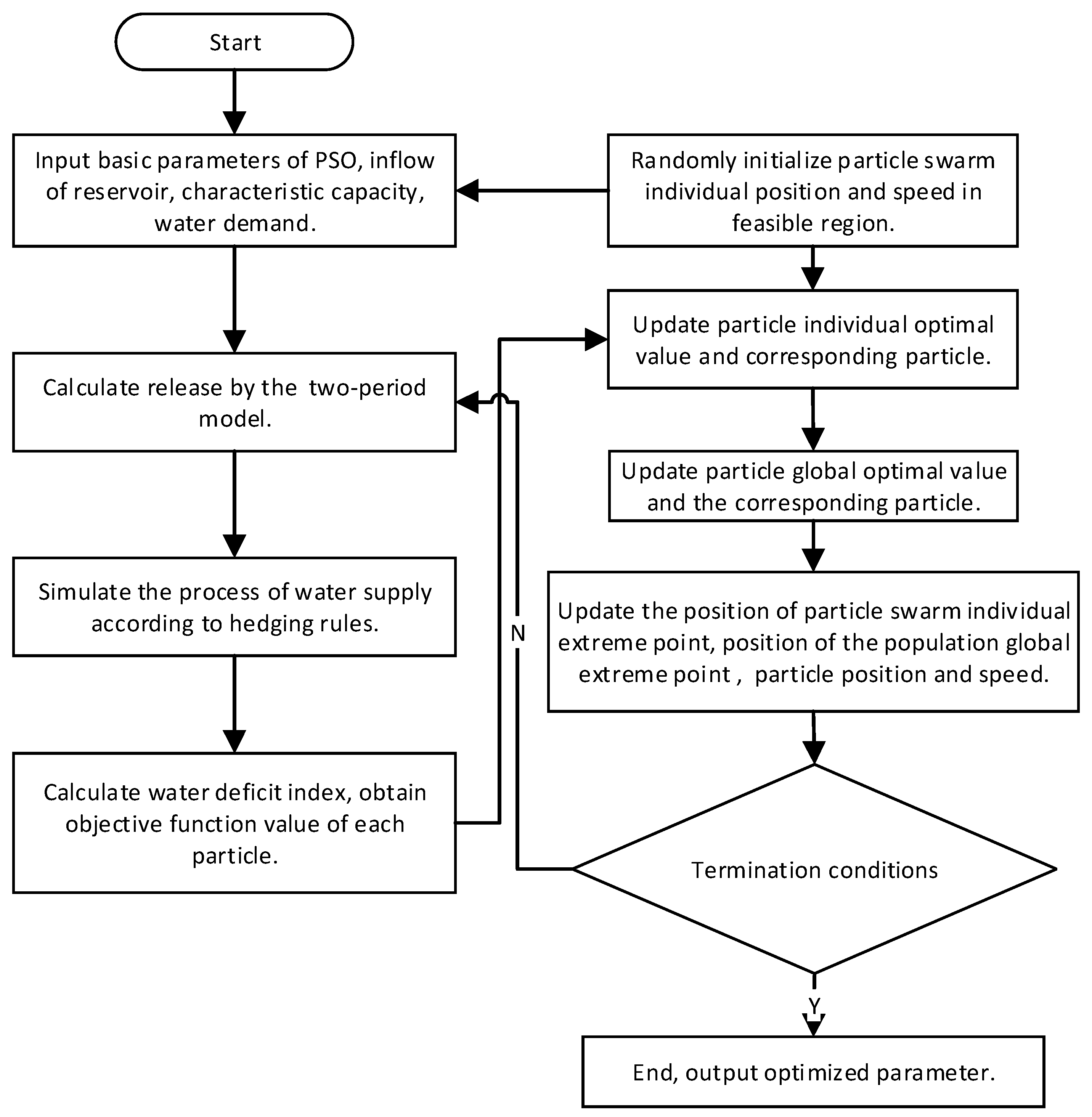
Water supply decision in a certain period can change the reservoir storage condition at the beginning of the next period, which affects the water supply decision in the next period and eventually influences the overall benefit of the reservoir in the long-series release. In order to ensure maximum long-term benefits, weighting factors and storage targets as the parameters need to be optimized by the simulation and optimization models. The structure of the models include state variable, decision variable, bound condition, and object function. The state variable is the reservoir storage and the decision variable is the reservoir release. The specific steps are as follows: (1) a set of parameters is randomly selected in the feasible region, the water supply process of the long-series is simulated through the two-period model, and the value of objective function is obtained; (2) according to the value of objective function, the parameters are adjusted by the optimization algorithm; (3) the water supply process of the long-series is simulated again after the readjustment of the parameters; and (4) repeat from step (1) to (3) again until a satisfactory value of the objective function is obtained. In this paper, one regulation cycle is separated into 12 regulation periods; the chosen parameters are the water storage target and the water supply weighting factor for each period w, which are 24 in total.
2.2.1. Objective Function
In order to allocate limited water resources between different regulation periods and avoid severe damage during some periods, the minimum shortage index (SI) is chosen as the objective function:
2.2.2. System Constraint
- (1)
- (2)
- (3)
Reservoir capacity constraint
where,
Sd is the dead storage capacity and
Su is the storage capacity of the reservoir.
2.2.3. Model Calculation
Parameter simulation and optimization models of hedging rules firstly determine a group of decision variables by use of the particle swarm optimization algorithm (PSO). Hedging rules can guide reservoir operation by this group of decision variables. The process of water supply is simulated in each period. The final statistical index uses the SI as the fitness value, and decision variables are readjusted by the PSO. Parameter simulations and the optimization model repeat the above steps again until the objective satisfies the requirements. The process is shown in
Figure 5.
3. Case Study
The developed model is applied to the Heiquan reservoir. The Heiquan reservoir is the most important water resource for Xining City, which is located in the Qinghai Province of China. The Heiquan reservoir was built in 1996 with a normal storage capacity of 124 million m3 and a dead storage of 17 million m3. Water demand has shown an upward trend along with the rapid development of the economy, which leads to the severe shortages of the Heiquan reservoir. To evaluate the HR rule, 55 years of monthly inflow data of the Heiquan reservoir is used from 1956 to 2010, resulting in a total of 660 months. The input data include reservoir properties, evaporation, and seepage of the reservoir.
In order to verify the feasibility of HR, which is composed of the two-period model and the parameter simulation optimization model, three kinds of comparable operation models are established, including standard operation policy (SOP), operation chart, and dynamic programming. The decision interval of solution process of the different operation model is one month in this study. The water shortage index (SI) and water supply damage recovery index (RI) are chosen as indexes, in order to evaluate scheduling results of the operation schemes. RI refers to average frequency of recovering from a water-deficiency condition during the operation period. RI is usually measured by the maximum number of successive water-deficiency periods in which the water supply degree is less than ADD for a risk analysis. The number of successive water-deficiency periods is fewer, the recovery ability is stronger. Conversely, the recovery ability is weaker.
3.1. Reasonable Analysis of Optimized Parameter
3.1.1. Impact Analysis of Parameters of HR
(1) Impact analysis of ω on HR
Equation (10) shows that the optimal reservoir release at time
t (
) is a function of η
t, when the carryover storage target at time t (
) is fixed. The derivative of the Equation (10) is calculated with respect to η
t, the result of derivation is as follows:
During the hedging period, WA cannot completely meet the benefit of storage and release, namely . According to the Equation (16), it shows that function about ηt is monotonically decreasing. While the result that ηt is monotonically decreasing with ω in the range of 0 to 1 can be determined from Equation (9). As a result, is monotonically increasing with ω during the hedging period, which indicates that ω is an important parameter for measuring current water supply.
Table 1 shows that ω does not have impact on EWA and SWA of HR in situation I and III, only influences that in situation II. The SWA of situation II is
, so
decreases with η
t during the hedging period. However, η
t decreases with ω in the range of 0 to 1. So,
is positively associated with ω, namely,
increases with
during the hedging period.
(2) Impact analysis of storage target on HR
Equation (8) shows that the optimal reservoir release at time
t (
) is a function of the carryover storage target at time t (
), when ω is fixed. The derivative of the Equation (8) is calculated with respect to
, the result of derivation is as follows:
Equation (17) shows that decreases with the increase of when during the hedging period. increases with the increase of when during the hedging period. When , monotonically decreases with the increase of , has no effect on .
The carryover storage target at time
t (
) mainly influences the EWA of the HR. The larger
is, the larger the hedging interval will be; otherwise, the hedging interval will be smaller.
Table 1 shows that
does not have impact on SWA of HR.
3.1.2. Rationality Analysis of Results of Optimization Parameters
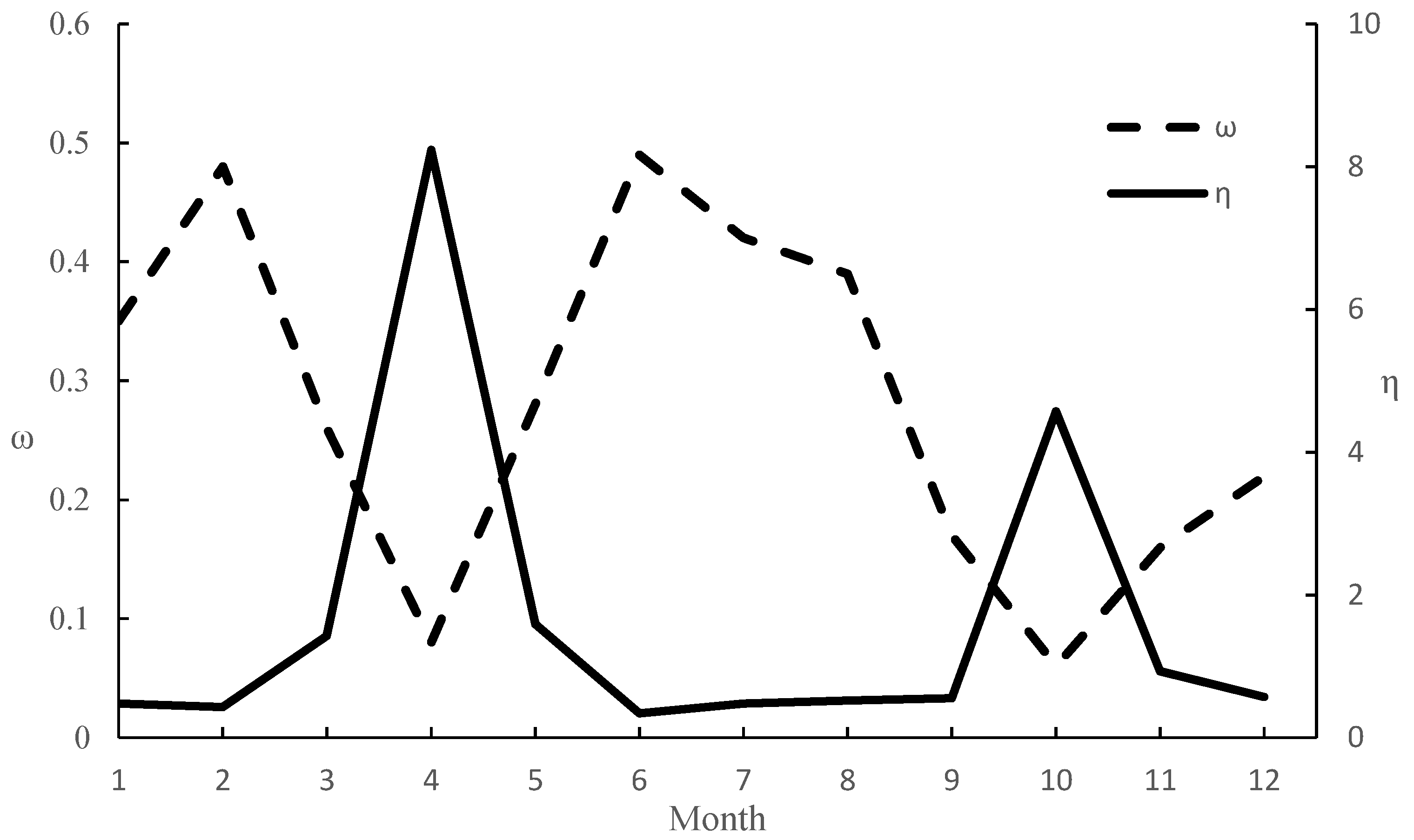
The optimal values of ω and η
t are shown in
Figure 6. It shows that ω is negatively correlated with η
t. Both ω and η
t show large fluctuations in scheduling period.
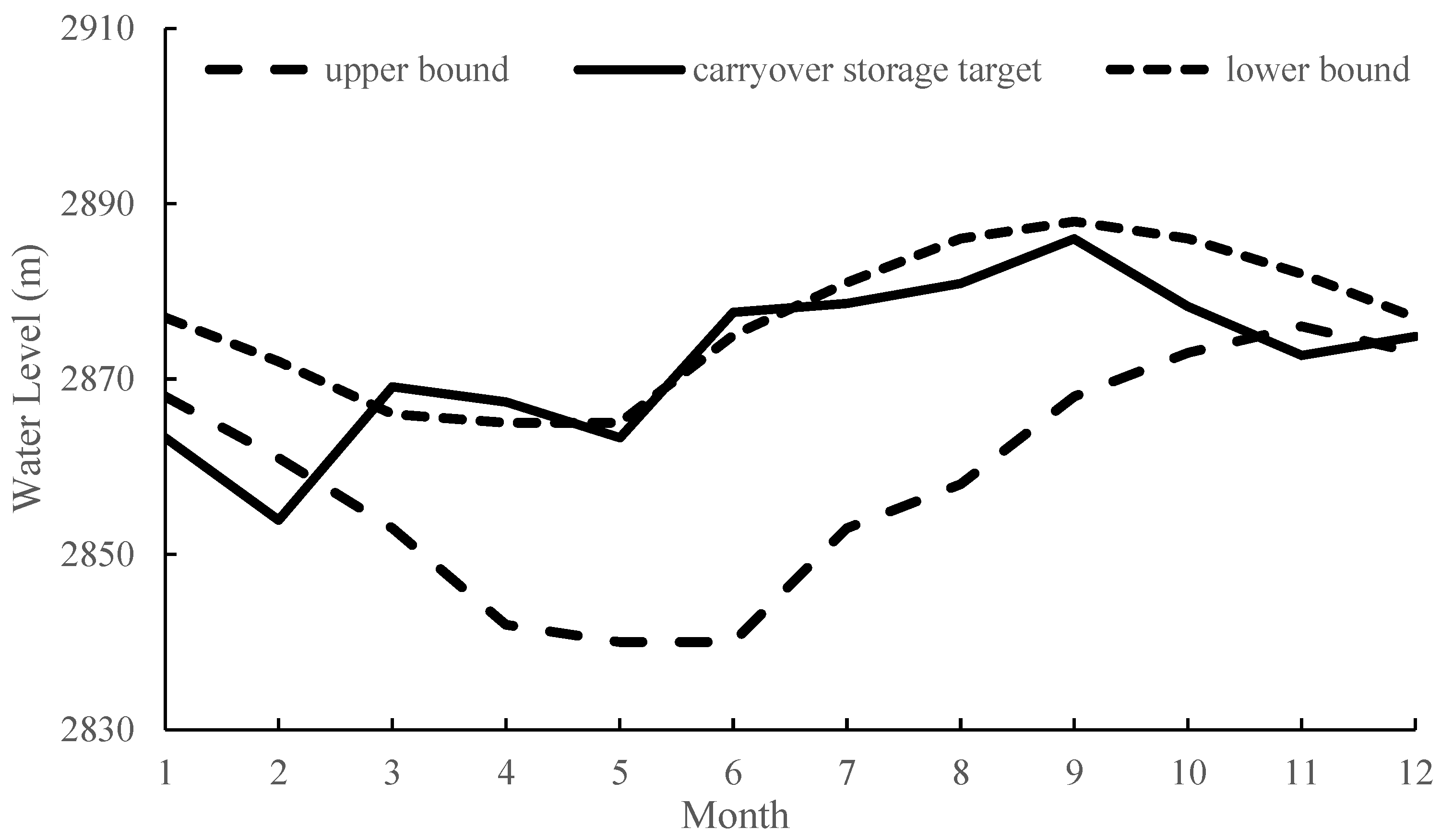
Figure 7 shows the change of the storage target in scheduling period. The upper bound and the lower bound represent operation lines of the operation chart. The upper bound and the lower bound are selected as the reference values for the rationality analysis of the storage target. In order to make a concrete analysis, the operation process is divided into three periods.
While the value of ω has a gradual increasing trend, the storage target changes smoothly from Novermber to Feburary in the following year. In this period, ω is smaller than 0.5, ηt is smaller than 1, and the storage target is mostly under the lower bound. It shows that the satisfaction degree of the release target is larger than that of the storage target in this period. In this period both the reservoir inflow and water demand is less, because this period is in the dry season, and there is no water supply for agriculture. Thus, water stored in the flood season can be used to avoid water supply damage in the beginning of this period. Consequently, the carryover storage target should be kept at a lower level to reduce the hedging water supply interval. With the decrease of stored water in the flood season, it is necessary to increase the water supply by increasing the value of ω during the hedging period.
There has been a high level of water demand from March to August; this period is called the constant water supply period (CWSP). The reservoir inflow also increases during the CWSP. The storage target decreases gradually, but it is higher than the upper bound in the first half of the CWSP (from March to May). The value of ω is smaller than that in the last period and ηt is larger than 1. Although reservoir inflow is increasing, water demand is higher than reservoir inflow in this period. Constant water supply can lead to the decrease of reservoir storage. Therefore, in order to avoid water supply damage, it is necessary to reduce the hedging water supply interval by decreasing the storage target. However, the satisfaction degree of release target is smaller than that of the storage target by decreasing the value of ω in this period, so that water is stored to avoid severe damage in the next period in advance.
The storage target increases gradually in the second half of the CWSP (from June to August). The value of ω is larger than that in the first half of the CWSP and ηt is smaller than 1. The flood season is the period from June to August, and the reservoir inflow is higher than water demand in this period. The increase of storage target is beneficial for water supply in the next period. Water demand needs to be satisfied as much as possible in this period. Increasing the value of ω can make the satisfaction degree of the release target higher than that of the storage target.
September and October are two special months. In September, inflow is higher, and water demand is lower. On the contrary, inflow is lower, and water demand is higher in October. The storage target is highest in September, ηt is smaller than 1. This allows for water to be stored in September, and the satisfaction degree of the release target is larger than that of the storage target. Oppositely, the storage target decreases in October, but still remains at a higher level, and ηt is larger than 1. Water is stored to avoid severe damage at the beginning of dry season.
3.2. Rationality Analysis of Hedging Rules
Table 2 and
Table 3 show the statistical results of water supply index of the four operation schemes. The statistical results show that the index result of dynamic pragramming is the most optimal. Dynamic pragramming is one optimum model; it divides the reservoir storage process into several parts, utilizes a step-by-step inducing principle to make decisions on every part, and then gets the optimistic operation performance of the total problem. The inflow condition is not taken into account under the SOP rule. The operation performance under the SOP is the worst with SI of 0.81 and RI of 7. The SI of the SOP scheme is the largest among the four schemes, which shows that the average degree of water supply is lower than that of other schemes. Meanwhile, there are 101 periods in which the water supply degree is less than ADD, accounting for 15.3% of the total periods. The proportion of the successive water-deficiency periods (≥2∆T) is the largest during these periods, accounting for 85.1% of the water-deficiency periods. This water supply policy is not suitable for the water supply in the dry season.
The operation performance under the operation chart is better than that under SOP with SI of 0.74 and RI of 6. The operation curves is obtained on the basis of analysis of the long-series inflow in the operation chart scheme. Consequently, operation curves can guide the reservoir to take measures to decrease water supply before the low water period. The water can be stored in advance to avoid water-deficiency, it proves that the SWA of the operation chart scheme is more reasonable. However, due to the operation feature of the operation chart scheme, the hedging coefficient of this model is fixed, and the hedging release is not optimal. There are 88 periods in which the water supply degree is less than ADD, accounting for 13.3%. That is a significant difference between the operation performance under the operation chart and that under dynamic prigramming.
The minimum SI is chosen as the objective function in the parameter simulation and optimization model, so the value of SI under HR is close to the value of SI under DP. The main advantage of the HR scheme is that the number of water-deficiency periods under HR is very close to that under DP. The results show that HR scheme is optimal except the DP scheme.
To analyze the reason for water deficiency and the operating features of the different operation schemes in the extreme dry season, this study chose two successive water-deficiency periods in the SOP scheme (October 1991–April 1992, January 1978–June 1978) for research.
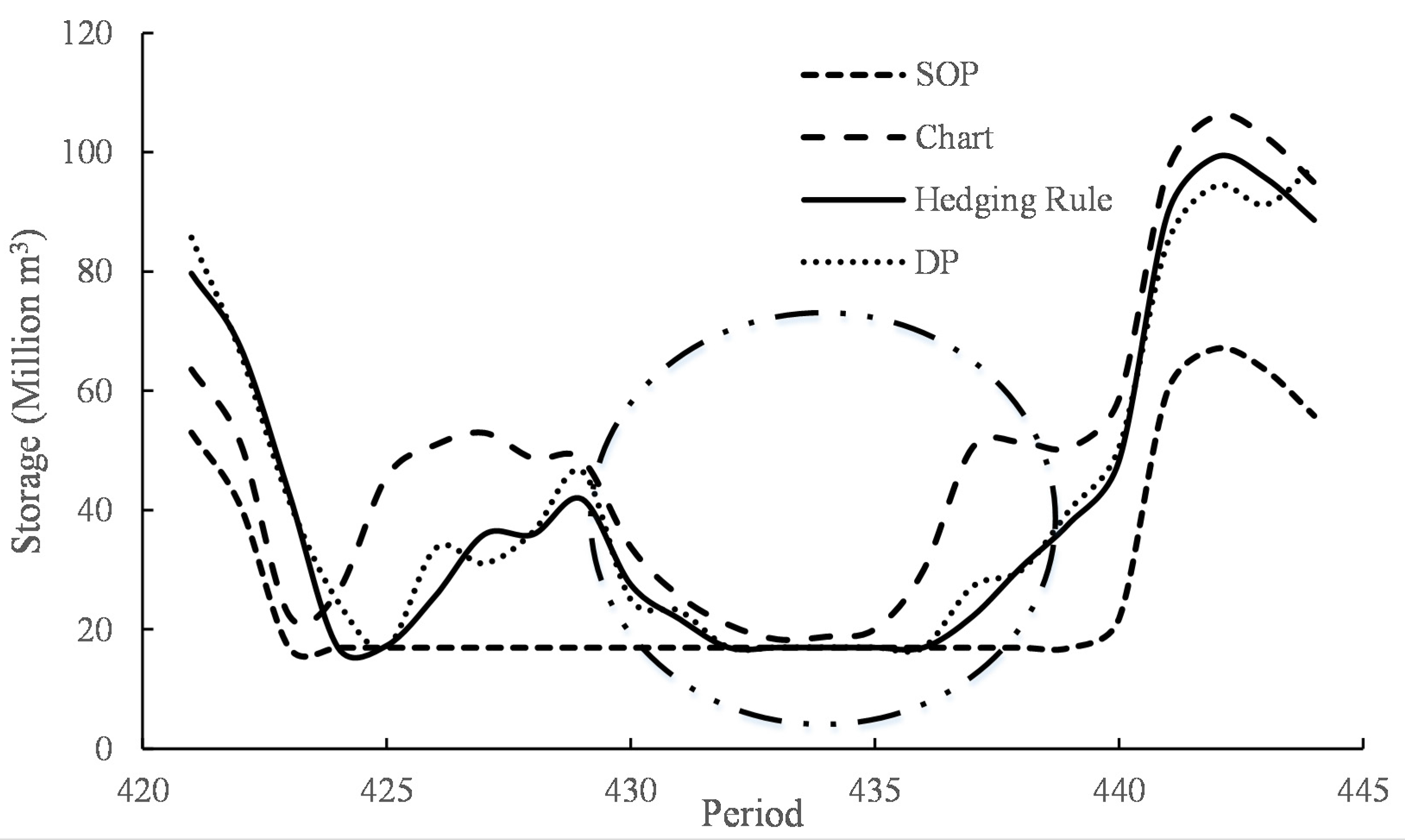
The longest successive water-deficiency periods occurred in Period 430–436 (October 1991–April 1992). The changing process of reservoir storage in period 421–444 (January 1991–December 1992) is shown in
Figure 8. Water is impounded in advance in Period 425–429 under the scheduling chart and HR before the successive water-deficiency period. The inflow level is far below the average, the total inflow of this period is 39.42 million m
3, and the average inflow is 80.88 million m
3. Water stored in advance fails to meet the water demand in this successive water-deficiency periods.
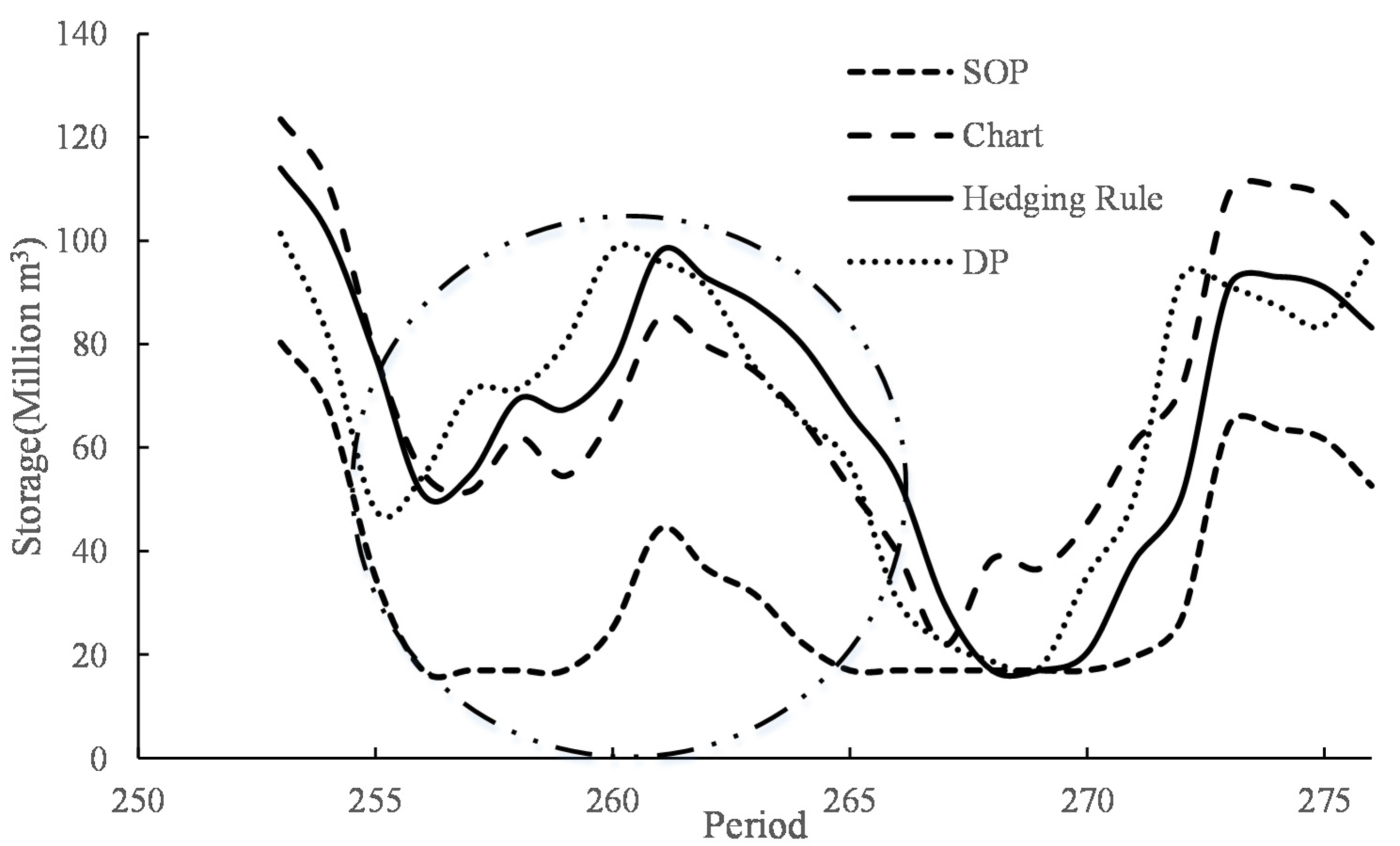
A successive water-deficiency period from January 1978 to June 1978 lasted six months under the SOP rule, lasted one month under scheduling chart, and zero months under the hedging rule. As a result, selecting the period from January 1977 to December 1978 (Period 253–276) for research, the changing process of reservoir storage during this period is shown in
Figure 9. Before the successive water-deficiency period, water is impounded in advance in Period 256–262 under the scheduling chart and HR. The reservoir stores water only at the end of flood season (Period 260–262) under the SOP rule. Thus, the storage water under the operation chart and HR is more than that under SOP at the beginning of the successive water-deficiency period (Period 263). In addition, the water supply hedging coefficient is fixed under the scheduling chart, so water supply cannot be adjusted according to the dry season. Water stored in advance cannot satisfy water supply requirement in the successive water-deficiency period, leading to deep damage. HR can guide the reservoir to carry out different levels of hedging the water supply at different periods by optimal reservoir release and avoid the deep damage better.
4. Conclusions
It is essential to develop the reasonable HR model for water supply reservoirs. This study proposed the hedging rule model which is composed of the two-period model and the parameter simulation and optimization model. The HR model contains two types of undetermined parameters. The undetermined parameters are optimized by the parameter simulation and optimization model. In order to verify the effectiveness of the HR model, the Heiquan reservoir is employed as a case study. The kinds of comparable operation models are developed, including standard operation policy (SOP), operation chart, and dynamic programming. Through comparing the operation performance of the models, the results are summarized below:
(1) The values of the optimal parameters have a larger fluctuation in a scheduling cycle, including the weighting factor and the storage target. The optimal parameters are proved reasonable by analyzing the inflow and water demand and can be used to guide the water supply; and
(2) The result shows that the operation performance of HR is close to that of DP and is better than that of the operation chart and SOP. The operation curves are obtained on the basis of analysis of the long-series inflow under the operation chart, so the result of the operation chart is superior to that of SOP. Due to the fixed hedging coefficient under the operation chart, the hedging release is non-optimized. The SWA, EWA, and hedging release are optimized in HR schemes, so the operation performances of HR is close to the optimal schemes.
Acknowledgments
This paper was jointly supported by National Key Technology R&D Program of the Ministry of Science and Technology (2013BAB05B05), National 973 project (2013CB036406).
Author Contributions
Yi Ji designed the experiments and wrote the manuscript; Xiaohui Lei provided suggestions on the data analysis and manuscript preparation, Siyu Cai and Xu Wang revised the manuscript.
Conflicts of Interest
The authors declare no conflict of interest.
References
- Zeng, X.; Hu, T.; Guo, X.; Li, X. Water transfer triggering mechanism for multi-reservoir operation in inter-basin water transfer-supply project. Water Resour. Manag. 2014, 28, 1293–1308. [Google Scholar] [CrossRef]
- Peng, Y.; Chu, J.; Peng, A.; Zhou, H. Optimization operation model coupled with improving water-transfer rules and hedging rules for inter-basin water transfer-supply systems. Water Resour. Manag. 2015, 29, 3787–3806. [Google Scholar] [CrossRef]
- Birhanu, K.; Alamirew, T.; Dinka, M.O.; Ayalew, S.; Aklog, D. Optimizing reservoir operation policy using chance constraint nonlinear programming for Koga irrigation Dam, Ethiopia. Water Resour. Manag. 2014, 28, 4957–4970. [Google Scholar] [CrossRef]
- Jothiprakash, V.; Shanthi, G. Single reservoir operating policies using genetic algorithm. Water Resour. Manag. 2006, 20, 917–929. [Google Scholar] [CrossRef]
- Maass, A.; Hufschmidt, M.M.; Dorfman, R.; Thomas, H.A., Jr.; Marglin, S.A.; Fair, G.M. Design of water resource system. Soil Sci. 1962, 94, 135. [Google Scholar] [CrossRef]
- Bower, B.T.; Hufschmidt, M.M.; Reedy, W.W. Operating procedures: Their role in the design of water-resource systems by simulation analyses. In Design of Water Resource System; Maass, A., Hufschmidt, M.M., Dorfman, R., Thomas, H.A., Jr., Marglin, S.A., Fair, G.M., Eds.; Harvard University Press: Cambridge, MA, USA, 1962; pp. 443–458. [Google Scholar]
- Clark, E.J. Impounding reservoirs. J. Am. Water Work. Assoc. 1956, 48, 349–354. [Google Scholar]
- Revelle, C.; Joeres, E.; Kirby, W. The linear decision rule in reservoir management and design: 1, Development of the stochastic model. Water Resour. Res. 1969, 5, 767–777. [Google Scholar] [CrossRef]
- Tu, M.-Y.; Hsu, N.-S.; Tsai, F.T.-C.; Yeh, W.W.-G. Optimization of hedging rules for reservoir operations. J. Water Resour. Plan. Manag. 2008, 134, 3–13. [Google Scholar] [CrossRef]
- Draper, A.J.; Lund, J.R. Optimal hedging and carryover storage value. J. Water Resour. Plan. Manag. 2004, 130, 83–87. [Google Scholar] [CrossRef]
- Tu, M.-Y.; Hsu, N.-S.; Yeh, W.W.-G. Optimization of reservoir management and operation with hedging rules. J. Water Resour. Plan. Manag. 2003, 129, 86–97. [Google Scholar] [CrossRef]
- You, J.Y.; Cai, X. Hedging rule for reservoir operations: 1. A theoretical analysis. Water Resour. Res. 2008, 44, W01415. [Google Scholar] [CrossRef]
- You, J.Y.; Cai, X. Hedging rule for reservoir operations: 2. A numerical model. Water Resour. Res. 2008, 44, W01416. [Google Scholar] [CrossRef]
- Celeste, A.B.; Billib, M. Evaluation of stochastic reservoir operation optimization models. Adv. Water Resour. 2009, 32, 1429–1443. [Google Scholar] [CrossRef]
- Shiau, J.T. Analytical optimal hedging with explicit incorporation of reservoir release and carryover storage targets. Water Resour. Res. 2011, 47. [Google Scholar] [CrossRef]
- Bayazit, M.; Ünal, N. Effects of hedging on reservoir performance. Water Resour. Res. 1990, 26, 713–719. [Google Scholar] [CrossRef]
- Srinivasan, K.; Philipose, M. Effect of hedging on over-year reservoir performance. Water Resour. Manag. 1998, 12, 95–120. [Google Scholar] [CrossRef]
- Shiau, J.; Lee, H. Derivation of optimal hedging rules for a water-supply reservoir through compromise programming. Water Resour. Manag. 2005, 19, 111–132. [Google Scholar] [CrossRef]
- Zhao, T.; Zhao, J.; Lund, J.R.; Yang, D. Optimal hedging rules for reservoir flood operation from forecast uncertainties. J. Water Resour. Plan. Manag. 2014, 140, 04014041. [Google Scholar] [CrossRef]
- Zhao, T.; Zhao, J. Optimizing operation of water supply reservoir: The role of constraints. Math. Probl. Eng. 2014, 2014, 853186. [Google Scholar] [CrossRef]
© 2016 by the authors; licensee MDPI, Basel, Switzerland. This article is an open access article distributed under the terms and conditions of the Creative Commons Attribution (CC-BY) license (http://creativecommons.org/licenses/by/4.0/).


