Potential Impacts of Food Production on Freshwater Availability Considering Water Sources

Abstract

We quantify the potential impacts of global food production on freshwater availability (water scarcity footprint; WSF) by applying the water unavailability factor (fwua) as a characterization factor and a global water resource model based on life cycle impact assessment (LCIA). Each water source, including rainfall, surface water, and groundwater, has a distinct fwua that is estimated based on the renewability rate of each geographical water cycle. The aggregated consumptive water use level for food production (water footprint inventory; WI) was found to be 4344 km³/year, and the calculated global total WSF was 18,031 km³ H₂Oeq/year, when considering the difference in water sources. According to the fwua concept, which is based on the land area required to obtain a unit volume of water from each source, the calculated annual impact can also be represented as 98.5 × 10⁶ km². This value implies that current agricultural activities requires a land area that is over six times larger than global total cropland. We also present the net import of the WI and WSF, highlighting the importance of quantitative assessments for utilizing global water resources to achieve sustainable water use globally.

1. Introduction

Water is a vital resource for human health, personal livelihoods, and quality of life. As recent water demand, especially in the agricultural sector, faces numerous challenges related to freshwater availability [1,2,3], quantifying the impacts of agricultural water use on freshwater availability is critical to improving sustainable water management. In regards to freshwater sustainability, the terrestrial renewable fresh water supply (RFWS_land) component has been proposed in the literature, and the human appropriation of accessible RFWS_land has been estimated at 30% [4]. The planetary boundary concept states that limitations on global freshwater use range between 1100 and 4500 km³/year [5,6]. These methods are based on the simple aggregated values of freshwater resources and their use; however, renewable freshwater resources exhibit spatiotemporal variability [7,8], implying that the potential environmental impacts of water use on freshwater availability also exhibit spatiotemporal variability. This finding shows that freshwater sustainability should be assessed in consideration of geographical distributions.

On the other hand, numerous studies have been conducted on the virtual flow of water through the international trade of food and other commodities. The virtual water concept has been developed to explain the virtual use of water through trading [9], and is has been adopted to estimate water dependency levels in countries using net virtual water imports [10]. Since the concept’s establishment, water savings through international trade have been estimated globally [11,12,13]. Recently, global virtual water transfer has been associated with the trade of agricultural and industrial products [14,15]. Virtual water flow volumes can be used to estimate the global balance between water supply and demand and the volume of water that is compensated through international trade. However, the virtual flow of water should also be assessed in consideration of the geographical distribution of water resources for the sustainable trade of virtual water.

Some key technical terms and an influential proposal on water footprint assessment (WFA) and life cycle assessment (LCA) related to water have been introduced [16,17]. The International Organization for Standardization (ISO) defines the “water footprint” as a metric that quantifies potential impacts related to water. According to the ISO 14046, a summation of water use is referred to as a “water footprint inventory (WI)” [18]. Several methods have been proposed to estimate the potential environmental impacts of changes in water quantities. The groundwater footprint (GF) has been presented as an estimate based on the potential impacts of groundwater use in major groundwater basins, which is represented by the area needed to sustain groundwater use and groundwater-dependent ecosystem services [19]. The water stress index (WSI) is derived from the ratio of water withdrawals to freshwater availability and from a variation factor weighted by the spatial precipitation distribution [20]. While these methods consider geographical distributions of water resources, different water sources are not addressed (i.e., only groundwater use for the GF and the aggregation of surface water and groundwater for the WSI). As each water source is uniquely renewable and available, the potential impacts of water use also vary by water source. The water unavailability factor (fwua) has been proposed as a means of characterizing water consumption based on its potential impacts, reflecting differences in water renewability levels according to place and water source [21]. Yano et al. [21] also conducted a case study to describe global food trade patterns via LCIA. However, the study was not based on the latest statistics or on multiple forcing datasets, and it did not involve a detailed discussion of country-based assessments of food production. In this study, we quantify the potential impacts of global food production on freshwater availability based on a detailed grid and country based evaluation. We assess the impact of international food trade from a LCIA perspective on sustainable water consumption, and we use the fwua concept, new trade statistics, and several forcing datasets to improve the robustness of the results.

2. Materials and Methods

2.1. Calculation of the Water Footprint Inventory

In this study, the WI of food production is defined as the total evapotranspiration from croplands during the cropping period of each agricultural product. Water use for fertilizers, pesticides, and machine production is not considered. To estimate the WI for agricultural and livestock production, the H08 model, a global water resources model, was used [22]. As this model addresses the effects of human activities (e.g., reservoir operation and cropland irrigation), while considering different types of water sources, the geographical distributions of water resources and differences between water sources can be counted for in the calculation of WI. Water and heat balance calculations made at a daily interval reflect the temporal aspect if the renewability rate of water resources and water usage from each source. Meteorological forcing data, including air temperature, surface pressure, rainfall rate, snow fall rate, wind speed, radiation, and specific humidity level, are adopted as climatic input data at daily intervals. River basins are expressed based on the elevation and flow direction. Cropland and irrigated area are considered based on the global dataset [23,24]. The WI values of 58 major trade commodities in consideration of different water sources (i.e., precipitation, stream flow, medium-sized reservoirs, and non-renewable and non-local blue water (NNBW)) are calculated at a resolution of 0.5° × 0.5°. NNBW is defined as a conceptual water source, and the WI of NNBW is defined as a component of water withdrawal that cannot be explained within the system boundaries. NNBW can be described as components of deep groundwater, lakes, glaciers, water diversions, and desalinated water that are not modelled in the H08 [12]. The NNBW value is known to be comparable to withdrawals reported for several aquifers in arid regions in the United States [12]. In this study, irrigated water from stream flows and medium-sized reservoirs are defined as the WI for surface water, and the irrigated NNBW value is defined as WI for groundwater.

WI flows were estimated for 58 major trade commodities derived from five major crops (i.e., barley, maize, rice, soy, and wheat) and three livestock products (i.e., beef, chicken, and pork) using FAOSTAT trade matrix data [25] (Table S1). The simulation settings used to calculate WI and WI flows were identical to those used in a previous study [10], although the meteorological forcing data and calculation period used differed. WATCH forcing data (WFD) [26], the third Global Soil Wetness Project (GSWP3) dataset [27], and Princeton’s Global Meteorological Forcing Dataset (PFD) [28] were used as input data for calculating the average WI for croplands between 1991 and 2000. As the WFD covers the period running to 2000, the GSWP3 and PFD were used to calculate the WI for between 2001 and 2008. The average WI for each agricultural product between 1991 and 2000 was used to determine WI flows between 22 regions.

2.2. Water Scarcity Footprint Assessment

The calculated WI was converted into a WSF by multiplying the value by a characterization factor. As the fwua was developed to characterize the WI in consideration of different water sources, we used the fwua as the characterization factor for this study [21]. The fwua was devised by Yano et al. [21]. For the readers’ convenience, the factor is described in brief below. See Yano et al. [21] for a detailed account and for the full formulation. The WSF of food production was determined as follows:

$$WSF={\displaystyle \sum _x\sum _l}\left(fwu{a}_{x,l}\times W{I}_{x,l}\right)$$

(1)

$$fwu{a}_{x,l}=\frac{A_{x,l}}{A_{ref}}$$

(2)

where x denotes the water source (including precipitation, surface water, and groundwater); fwua is based on the land area required to obtain the reference volume of water from each water source; A_x,l is the required land area per unit of time to obtain the reference volume for water from water source x at location l; and A_ref is the required land area per unit of time to obtain the reference volume of water from the reference condition [21]. In this study, the reference volume is defined as 1 m³ of rainfall per year over an area of 1.0 m² (e.g., 1000 mm/year) based on the global mean annual precipitation level. The calculated WSF has global mean precipitation equivalent units (e.g., m³ H₂Oeq). The fwua value for precipitation was calculated from the average annual precipitation for each domain using WFD, GSWP3, and PFD. The fwua values for surface water and groundwater were calculated from the average total runoff and sub-surface runoff levels of each domain using WFD, GSWP3, and PFD according to H08. All factors have a spatial resolution of 0.5° × 0.5°. The calculation period was identical to that used to determine the WI. The fwua values adopted herein do not account for the effects of water inputs from upstream regions, thus allowing the WSF to be assessed based on local water consumption levels. To prevent extremely high fwua values from increasing the total WSF, upper limits were defined at the 99th percentiles of each fwua. The upper fwua values for rainfed cropland precipitation, irrigated cropland precipitation, surface water, and groundwater were 5.0, 5.0, 100, and 200, respectively, for the study period.

3. Results

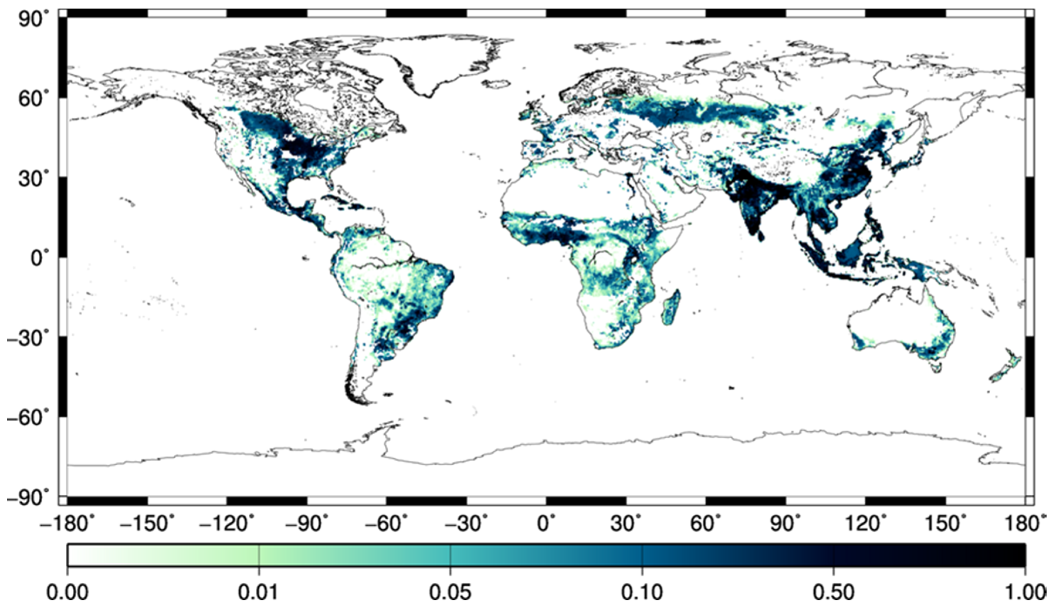
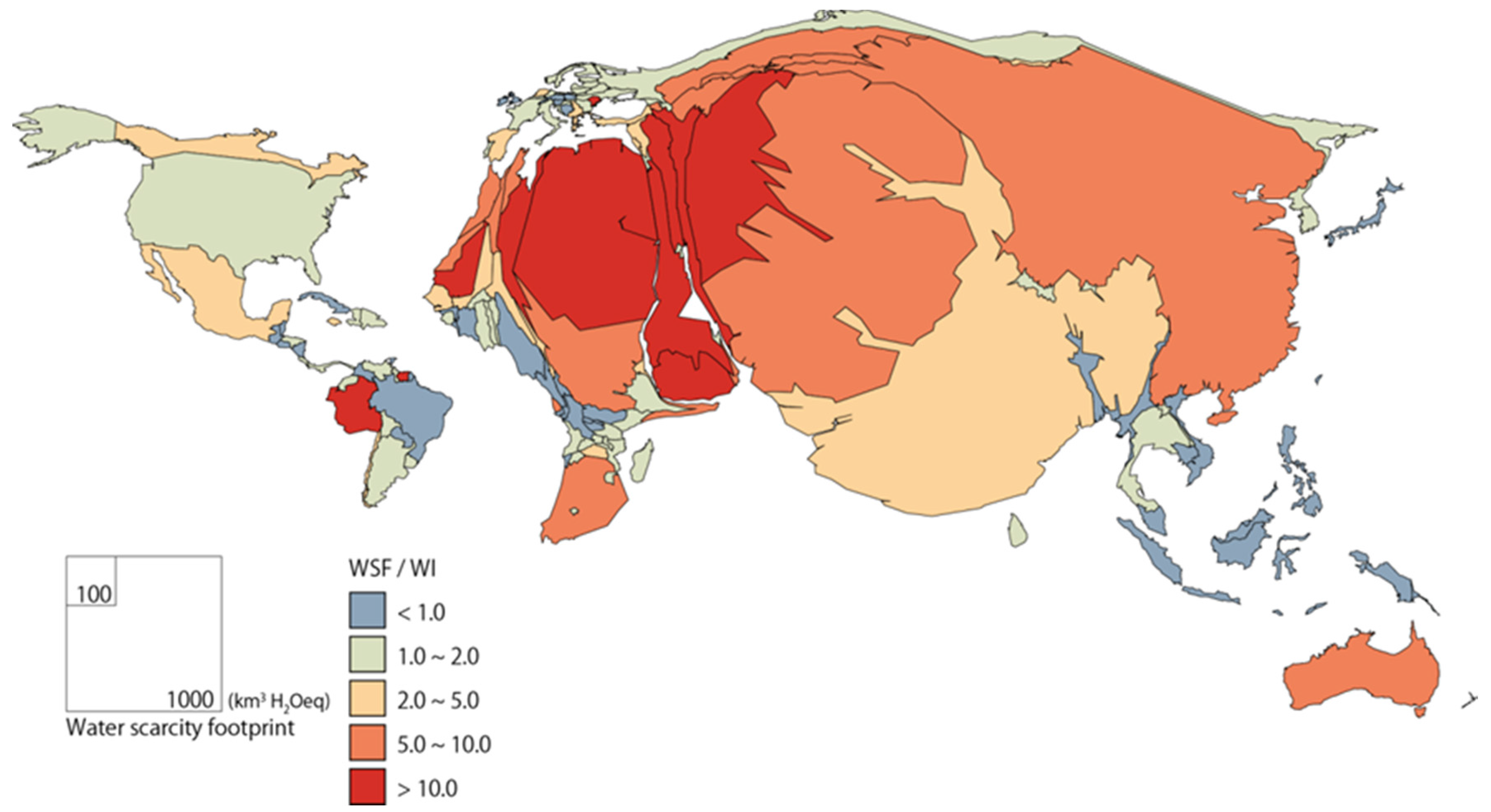
3.1. Water Footprint Inventory and the Water Scarcity Footprint of Global Food Production

The global total WI related to global agricultural activities is shown in Figure 1 and in Tables S2 to S3. The total globally averaged WI reached 4344 km³/year between 1991 and 2000, and 4592 km³/year between 2001 and 2008. According to the t-test results that assume that two average values are equal in a null hypothesis, the p- value of the average values for the two periods was 0.6; therefore, differences between the WI results are not statistically significant. According to the individual water sources, the WI of precipitation in rainfed croplands accounted for more than 50 % of the total WI. India, China, the United States, Pakistan, and Indonesia generated the highest WI values during this period, i.e., 790, 571, 484, 252, and 244 km³/year, respectively. These five countries accounted for approximately 50% of the total global WI.

The global total WSF related to agricultural activities reached 18,031 km³ H₂Oeq/year between 1991 and 2000, and 21,673 km³ H₂Oeq/year between 2001 and 2008 (Tables S4 and S5). The WSF results for all water sources were greater than the WI values for these periods. Between 1991 and 2000, the WSFs for rainfed cropland precipitation, irrigated cropland precipitation, surface water, and groundwater were 1.2, 1.2, 7.7, and 21.2 times greater than the WI values, respectively. Although the WI for groundwater constituted only 8.5 % of the total WI, the WSF for groundwater accounted for 43.4 % of the total WSF. The highest WSF value was registered at 24.25° N, 33.25° E in Egypt. The WSF for groundwater reached 42.6 km³ H₂Oeq/year, accounting for 95% of the total WSF of this domain. The fwua value for groundwater in this domain reached 171. This grid belongs to the Nubian Sandstone aquifer, which was reported as a non-renewable aquifer system [29]. Central America, India, Pakistan, Northern China, and Southeastern Australia registered high WSFs. Figure 2 shows the annual WSF and the WSF/WI ratio for each country between 1991 and 2000; the image was visually enhanced using a cartogram [30]. The area of each country is proportionate to the WSF map, and boundary lines have been maintained. Countries dependent on minimal renewable water resources are represented as large countries in this figure. China, India, Pakistan, the United States, and Egypt registered the highest WSFs, i.e., 3415, 2061, 2408, 922, and 892 km³ H₂Oeq/year, respectively. Saudi Arabia, Libya, Yemen, and Egypt registered the highest WSF/WI ratios, i.e., 44.5, 38.2, 25.8, and 25.2, respectively. The Middle East and North African (MENA) countries tended to generate high WSF/WI ratios. Outside of the MENA region, Suriname and Chile registered WSF/WI ratios exceeding a value of 10. By contrast, Southeast Asia, Japan, Central Africa, and Brazil registered small areas with WSF/WI ratios of less than 1.0. The ratio of the WI for groundwater to the total WI for Brazil was founded to be less than 0.1%, whereas a value of 34.5% was found for Egypt.

The WSF results divided based on cropland areas within each country and basin (mm H₂Oeq/year) are shown in Figures S3 and S4. While the country-based results can be easily applied for assessment purposes using country-based statistical data, the basin-based results do not require one to consider the effects of water inputs from upstream areas of international river basins. The total WSF value for the United States reached 507 mm H₂Oeq/year (including 553 mm H₂Oeq/year for the Mississippi River, the largest basin in the country). The WSF of the Colorado River reached 4261 mm H₂Oeq/year, exceeding the national average value. As the cropland area of the river basin accounted for only 1.1% of the total cropland area for the US, Colorado River basin had a minor effect. For the countries with large cropland areas, the WSF values of local basins were more suited to sustainability assessments of local water issues.

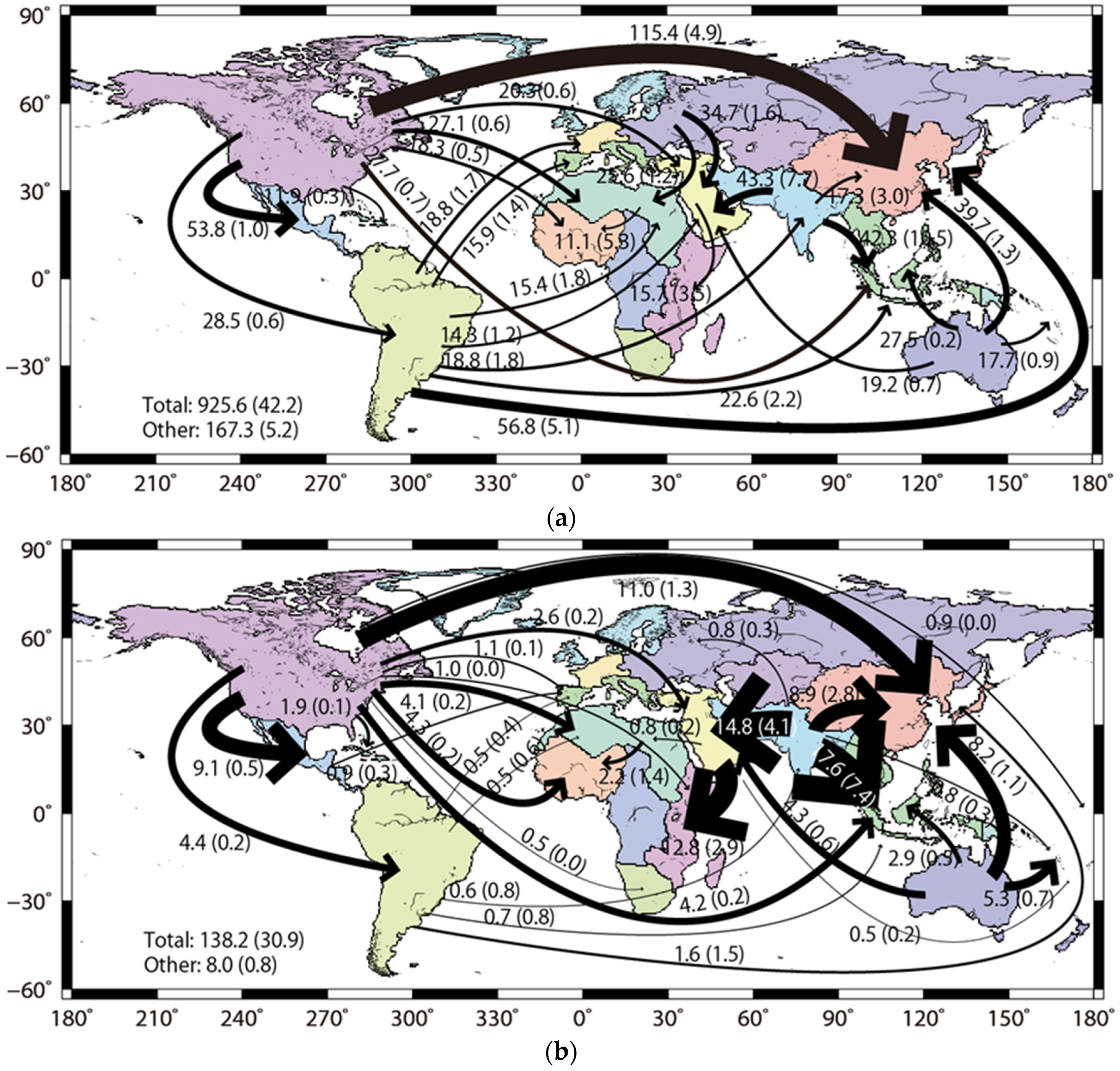
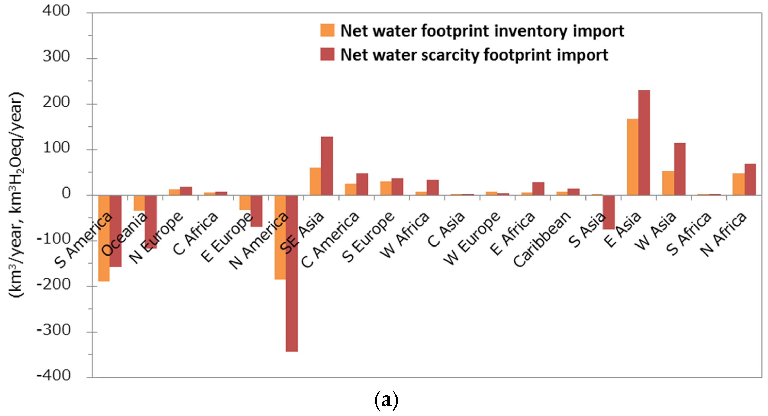
3.2. Water Scarcity Footprint Flows Based on Food Trade

WSF flows from 2010 that were divided by country were aggregated into 22 regions based on a previous study [18]. Figure 3 shows (a) net exports of the WSF for all water sources and (b) irrigated groundwater alone. The “total” value represents the total net flows between the 22 regions, and “other” signifies the total flows below threshold values, i.e., 10 km³ H₂Oeq/year for all water sources and 0.5 km³ H₂O/year for irrigated groundwater. The numbers shown in parentheses are the standard deviations of the calculated values between the three meteorological forcing datasets. Global total net flows of WI between the 22 regions were calculated at 524.8 km³/year. Previous studies have estimated global gross flows of WI related to crop trades as 695 km³/year for 1995–1999 and global net exports as 355 to 545 km³/year for 2000 [12,21,31]. Although there is not full agreement between the simulation settings (the period, net and gross values, countries, and crops examined in this study), it appears that WI flows were adequately estimated. The WSF flows tended to generate larger arrows than the WI for both types of water sources. The total WSF flows were 1.8 times greater than the total WI flows. WSF water source, precipitation, surface water, and groundwater values were 1.1, 8.2, and 13.8 times greater than the WI values, respectively. In regard to each region, WSF flows for Northern Africa, Eastern Asia, Southern Asia, Western Asia, North America, and Oceania were 15.5, 15.6, 4.9, 11.7, 1.8, and 3.4 times greater than the WI values, respectively. In comparison, WSF flows for the Caribbean, South America, and Northern Europe were 0.6, 0.9, and 0.8 times greater than the WI values, respectively, and in these regions, food production levels were dependent on the presence of abundant water resources. North America, South America, Oceania, and Southern Asia were characterized by net exports of 345.4, 187.8, 118.6, and 109.1 km³ H₂Oeq/year, respectively, in 2010. Relative to previous case study results on WSF flows in 2000 [22], the imported value of the WSF for Eastern Asia has been increasing. The imported WSF from North America grew from 88.5 km³ H₂Oeq/year in 2000 to 115.4 km³ H₂Oeq/year in 2010 and that from South America increased from 12.6 km³ H₂Oeq/year in 2000 to 56.8 km³ H₂Oeq/year in 2010. This fact is mainly attributed to the growth of the Chinese economy. According to the FAO, the net importing value of crops and livestock products of China increased from 6.5 billion USD in 2000 to 55.4 billion USD in 2010.

The WSF/WI ratios for groundwater for North Africa, North America, South America, Eastern Asia, and Southern Asia were recorded as 18.5, 9.1, 27.7, 14.5, and 14.0, respectively. The largest flows of the WSF from groundwater were reached 46.4 km³ H₂O/year for North America, 43.8 km³ H₂Oeq/year for southern Asia, 21.3 km³ H₂Oeq/year for Oceania, and 14.5 km³ H₂Oeq/year for Western Asia. South America, which generated the second largest WSF flow for all water sources, registered a net WSF export level of only 5.3 km³ H₂Oeq/year for groundwater. This implies South America did not export food produced from scarce water resources, although large quantities of food produced from water sources with lower potential impacts were exported during the study period.

4. Discussion

The estimated global total WSF presents valuable information for understanding the sustainability of existing agricultural systems. As the fwua value is based on the land area required to obtain the reference volume of water, the WSF/WI ratio contains information on the required land area to maintain current agricultural conditions in terms of water availability. The WSF/WI ratio can also be described as a characterization factor weighted by the volume of water use. The WSF/WI ratios for rainfed cropland precipitation, irrigated cropland precipitation, irrigated cropland surface water, and irrigated cropland groundwater were calculated as 1.2, 1.2, 7.7, and 21.2, respectively. Rainfed and irrigated cropland areas covered 12.4 × 10⁶ km² and 2.8 × 10⁶ km² [23,24], respectively. The 18,031 km³ H₂Oeq/year value calculated for the WSF can also be referred to as 98.5 × 10⁶ km² of the required land area by multiplying each cropland area by the corresponding WSF/WI ratio. This value was 6.6 times greater than the 14.9 × 10⁶ km² value calculated for the total cropland area [23] and was 6.4 times greater than the 15.4 × 10⁶ km² value calculated for the total arable and permanent cropland area of 2010 [32].

Figure 4 shows the net WI and WSF import levels due to international food trade (exports are negative), the gross domestic product (GDP) per capita [33], and the ratio of irrigated croplands to cumulative croplands for each region. Melanesia, Micronesia, and Polynesia were excluded from the analysis, as these regions generated low proportions. As noted above, South America’s WSF value is smaller than its WI, implying that the region produced food using abundant water resources. In comparison, Oceania and North America generated larger WSFs relative to their WI values. Southern Asia was a net importing region in terms of its WI; however, it was a net exporting region in terms of its WSF. In other words, Southern Asia exports foods produced from scarcer water resources than the water resources used to produce imported foods. GDP per capita values serve as a justification for why Oceania and North America exported foods using scarce water resources. For example, a high GDP creates technological capacities to develop new water resources, to maintain high water-use efficiency levels, and to secure low water use costs due to the presence of competitive industry structures. However, Southern Asia exported food produced from scarce water resources due to the country’s high ratio of irrigated cropland. Southern Asia’s irrigated ratio reached 37%, exceeding values of 10% and 13% for Oceania and North America, respectively. This high ratio resulted in higher water-use efficiency levels, implying that the aggressive use of scarce water resources occurred in Southern Asia.

Figure 5 shows the renewable water resources [32] and WI per capita for each region. Although South America and Central Africa prevented abundant water resources per capita, the ratio of water utilization remained low. The sustainable use of water at a global scale requires the utilization of abundant water resources with lower potential impacts (especially in these regions) in consideration of supply, demand, and sustainable water use. This quantitative assessment of WI and WSF can contribute to strategies on how to utilize global water resources to achieve global sustainability. Domestic water resources may not be utilized adequately for the following reasons:

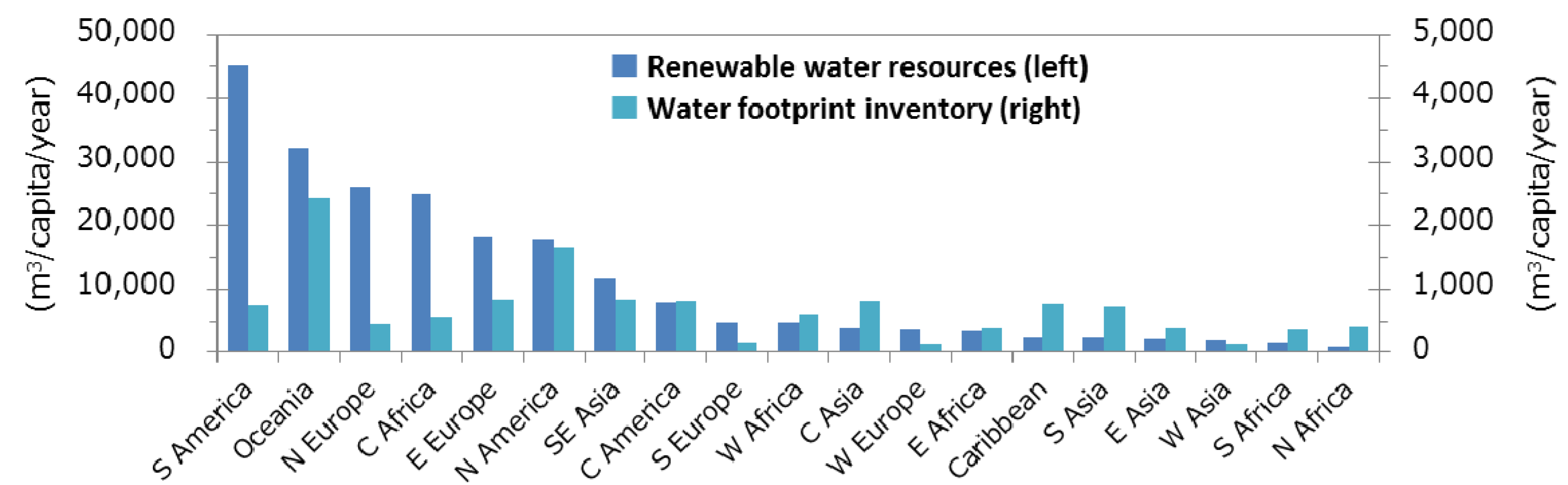
• Irrigated croplands are limited due to low GDP levels (e.g., South America and Central Africa), resulting in limited water resource utilization;
• Industrial structures have not been developed due to low GDP levels, which has led to minimal competitive and small-scale agricultural practices and low levels of water resource utilizations;
• Water resource development is difficult to achieve due to low GDP and low technological capacity levels, resulting in low water resource utilization;
• High costs of infrastructure use imply high costs for water use, resulting in low water resource utilization; and
• Climatic conditions are not conductive to intensive agriculture (e.g., Northern Europe [34]), causing individuals to not utilize domestic water resources adequately.

All of these phenomena are influenced by both social and natural factors. However, resolving uneven GDP distributions could effectively promote global water-use efficiency.

In regards to hydrological modelling, the state of current practices has been reviewed and the scientific and data-related challenges have been considered with a focus on human-water activities manifested through water resource management [35,36]. The H08 is used as one of the latest large-scale hydrological models to show how international trade helps control regional water demand. The results of our calculations include uncertainties due to modelling assumptions. In considering the uncertainties in meteorological forcing data, this study adopts an average result value using three meteorological forcing datasets. To evaluate uncertainties in groundwater withdrawal levels, we used the NNBW measure that has been validated as comparable to groundwater withdrawal levels reported for several arid aquifers. Although these results include uncertainties, this study presents new information and insights on water footprint and international food trade patterns from an LCA point of view. It is valuable to quantitatively assess the potential impacts of water use and virtual flows related to international food trade at a global scale in consideration of different water sources.

5. Conclusions

Potential impacts on global food production freshwater availability (WSF) and flows of WSF related to international food trade were estimated using the fwua, which reflects the difference in water renewability rates by source. The global WSF of food production reached 18,031 km³ H₂Oeq/year and was also described as 98.5 × 10⁶ km² of the required land area, which is equivalent to 4.2 times the value of the summation of the WI. Although groundwater constituted only 8.5% of the total WI, it accounted for 43.4% of the total WSF. China, India, Pakistan, the United States, and Egypt exhibited the highest WSFs, showing dependence on minimal renewable water resources. WSF flows via food trade are 1.8 times greater than the total WI flows. In total, 925.6 km³ H₂Oeq of WSF are traded each year. The WSF imported by Eastern Asia is growing mainly because of the rapid growth of the Chinese economy. Southern Asia is a net WI importing region, however, it is also a net WSF exporting region, which implies its dependence on scarcer water resources for food production rather than on water used to produce imported foods. Sustainable water use requires the utilization of abundant water resources at a global scale, and uneven GDP distributions can be resolved to effectively promote global water-use efficiency. The assessment of WSF showed a new insight that net WI importing regions can be net WSF exporting regions considering the difference in water sources. The results illustrate the importance of quantitative assessments of WI and WSF for utilizing global water resources to achieve global sustainability with lower potential impacts.

References

1. The 2030 Water Resources Group. Charting our Water Future: Economic Frameworks to Inform Decision-Making; McKinsey & Company: New York, NY, USA, 2009. [Google Scholar]
2. Foley, J.A.; Ramankutty, N.; Brauman, K.A.; Cassidy, E.S.; Gerber, J.S.; Johnston, M.; Mueller, N.D.; O’Connell, C.; Ray, D.K.; West, P.C.; et al. Solutions for a cultivated planet. Nature 2011, 478, 337–342. [Google Scholar] [CrossRef] [PubMed]
3. Food and Agriculture Organization of the United Nations (FAO). The State of the World’s Land and Water Resources for Food and Agriculture (SOLAW)—Managing Systems at Risk; FAO: Rome, Italy, 2011. [Google Scholar]
4. Postel, S.L.; Daily, G.C.; Ehrlich, P.R. Human appropriation of renewable fresh water. Science 1996, 271, 785–788. [Google Scholar] [CrossRef]
5. Rockström, J.; Stefen, W.; Noone, K.; Persson, A.; Chapin, F.S.; Lambin, E.F.; Lenton, T.M.; Scheffer, M.; Folke, C.; Schellnhuber, H.J.; et al. A safe operating space for humanity. Nature 2009, 461, 472–475. [Google Scholar] [CrossRef] [PubMed]
6. Gerten, D.; Hoff, H.; Rockström, J.; Jägermeyr, J.; Kummu, M.; Pastor, A.V. Towards a revised planetary boundary for consumptive freshwater use: Role of environmental flow requirements. Curr. Opin. Environ. Sustain. 2013, 5, 551–558. [Google Scholar] [CrossRef]
7. The United Nations Educational, Scientific and Cultural Organization (UNESCO). Managing Water under Uncertainty and Risk (Vol. 1); The United Nations World Water Development Report 4; UNESCO: Paris, France, 2012. [Google Scholar]
8. Hoekstra, A.Y.; Mekonnen, M.M.; Chapagain, A.K.; Mathews, R.E.; Richter, B.D. Global monthly water scarcity: Blue water footprints versus blue water availability. PLoS One 2012, 7, e32688. [Google Scholar]
9. Allan, J.A. Virtual water: A strategic resource global solutions to regional deficits. Groundwater 1998, 36, 545–546. [Google Scholar] [CrossRef]
10. Hoekstra, A.Y.; Hung, P.Q. Virtual Water Trade, A Quantification of Virtual Water Flows between Nations in Relation to International Crop Trade; Value of Water Research Report Series No. 11; UNESCO-IHE: Delft, The Netherland, 2002. [Google Scholar]
11. Aldaya, M.M.; Llamas, M.R. Water Footprint Analysis for the Guadiana River Basin; Value of Water Research Report Series No. 35; UNESCO-IHE: Delft, The Netherland, 2008. [Google Scholar]
12. Hanasaki, N.; Inuzuka, T.; Kanae, S.; Oki, T. An estimation of global virtual water flow and sources of water withdrawal for major crops and livestock products using a global hydrological model. J. Hydrol. 2010, 384, 232–244. [Google Scholar] [CrossRef]
13. Hoekstra, A.Y.; Mekonnen, M.M. The water footprint of humanity. PNAS 2012, 109, 3232–3237. [Google Scholar] [CrossRef] [PubMed]
14. Oki, T.; Kanae, S. Global hydrological cycles and world water resources. Science 2006, 313, 1068–1072. [Google Scholar] [CrossRef] [PubMed]
15. Mekonnen, M.M.; Hoekstra, A.Y. National Water Footprint Accounts: the Green, Blue and Grey Water Footprint of Production and Consumption; Value of Water Research Report Series No. 50; UNESCO-IHE: Delft, The Netherland, 2011. [Google Scholar]
16. Boulay, A.M.; Hoekstra, A.Y.; Vionnet, S. Complementarities of water-focused life cycle assessment and water footprint assessment. Environ. Sci. Technol. 2013, 47, 11926–11927. [Google Scholar] [CrossRef] [PubMed]
17. Manzardo, A.; Mazzi, A.; Loss, A.; Butler, M.; Williamson, A.; Scipioni, A. Lessons learned from the application of different water footprint approaches to compare different food packaging alternatives. J. Clean. Prod. 2016, 112, 4657–4666. [Google Scholar] [CrossRef]
18. International Organization for Standardization (ISO). ISO 14046 Environmental Management, Water Footprint—Principles, Requirements and Guidelines; ISO: Geneva, Switzerland, 2014. [Google Scholar]
19. Gleeson, T.; Wada, Y.; Bierkens, M.F.P.; van Beek, L.P.H. Water balance of global aquifers revealed by groundwater footprint. Nature 2012, 488, 197–200. [Google Scholar] [CrossRef] [PubMed]
20. Pfister, S.; Koehler, A.; Hellweg, S. Assessing the environmental impacts of freshwater consumption in LCA. Environ. Sci. Technol. 2009, 43, 4098–4104. [Google Scholar] [CrossRef] [PubMed]
21. Yano, S.; Hanasaki, N.; Itsubo, N.; Oki, T. Water Scarcity Footprints by Considering the Differences in Water Sources. Sustainability 2015, 7, 9753–9772. [Google Scholar] [CrossRef]
22. Hanasaki, N.; Kanae, S.; Oki, T.; Masuda, K.; Motoya, K.; Shirakawa, N.; Shen, Y.; Tanaka, K. An integrated model for the assessment of global water resources—Part 1: Model description and input meteorological forcing. Hydrol. Earth Sys. Sci. 2008, 12, 1007–1025. [Google Scholar] [CrossRef]
23. Ramankutty, N.; Evan, A.; Monfreda, C.; Foley, J.A. Farming the planet: 1. Geographic distribution of global agricultural lands in the year 2000. Glob. Biogeochem. Cycles 2008, 22. [Google Scholar] [CrossRef]
24. Siebert, S.; Doll, P.; Hoogeveen, J.; Faures, J.M.; Frenken, K.; Feick, S. Development and validation of the global map of irrigation areas. Hydrol. Earth Sys. Sci. 2005, 9, 535–547. [Google Scholar] [CrossRef]
25. The Food and Agriculture Organization Corporate Statistical Database (FAOSTAT). Available online: http://faostat.fao.org/ (accessed on 5 August 2014).
26. Weedon, G.P.; Gomes, S.; Viterbo, P.; Shuttleworth, W.J.; Blyth, E.; Österle, H.; Adam, J.C.; Bellouin, N.; Boucher, O.; Best, M. Creation of the WATCH forcing data and its use to assess global and regional reference crop evaporation over land during the twentieth century. J. Hydrometeorol. 2011, 12, 823–848. [Google Scholar] [CrossRef]
27. Kim, H.; Yoshimura, K.; Chang, E.; Famiglietti, J.S.; Oki, T. Century long observation constrained global dynamic downscaling and hydrologic implication. In Proceedings of the AGU Fall Meeting 2012, San Francisco, CA, USA, 3–7 December 2012; American Geophysical Union: Washington DC, USA, 2012. GC31D-02. [Google Scholar]
28. Sheffield, J.; Goteti, G.; Wood, E.F. Development of a 50-yr high-resolution global dataset of meteorological forcings for land surface modeling. J. Clim. 2006, 19, 3088–3111. [Google Scholar]
29. Arabi, N.E. Environmental Management of Groundwater in Egypt via Artificial Recharge Extending the Practice to Soil Aquifer Treatment (SAT). Int. J. Environ. Sustain. 2012, 1, 66–82. [Google Scholar]
30. Inoue, R.; Shimizu, E. A new algorithm for continuous area cartogram construction with triangulation of regions and restriction on bearing changes of edges. Cartogr. Geogr. Inf. Sci. 2006, 33, 115–125. [Google Scholar] [CrossRef]
31. Chapagain, A.K.; Hoekstra, A.Y. Virtual Water Flows between Nations in Relation to Trade in Livestock and Livestock Products; Value of Water Research Report Series No. 13; UNESCO-IHE: Delft, The Netherland, 2003. [Google Scholar]
32. AQUASTAT. Available online: www.fao.org/nr/aquastat/ (accessed on 23 July 2014).
33. World Economic Outlook Databases. Available online: http://www.imf.org/external/ns/cs.aspx?id=28 (accessed on 1 February 2014).
34. Maracchi, G.; Sirotenko, O.; Bindi, M. Impacts of Present and Future Climate Variability on Agriculture and Forestry in the Temperate Regions: Europe. Clim. Chang. 2005, 70, 117–135. [Google Scholar] [CrossRef]
35. Nazemi, A.; Wheater, H.S. On inclusion of water resource management in Earth system models—Part 1: Problem definition and representation of water demand. Hydrol. Earth Syst. Sci. 2015, 19, 33–61. [Google Scholar] [CrossRef]
36. Nazemi, A.; Wheater, H.S. On inclusion of water resource management in Earth system models—Part 2: Representation of water supply and allocation and opportunities for improved modeling. Hydrol. Earth Syst. Sci. 2015, 19, 63–90. [Google Scholar] [CrossRef]
Figure 1. Global distribution of the annual water footprint inventory related to food production between 2001 and 2008 (km3/year).
Water 08 00163 g001
Figure 2. The water scarcity footprint for each country (area size) and the ratio of the water scarcity footprint to the water footprint inventory (colour coded).
Water 08 00163 g002
Figure 3. Water scarcity footprint flows due to international food trade between 22 regions for (a) all water sources (exceeding 10 km3 H2Oeq/year) and (b) groundwater (exceeding 0.5 km3 H2Oeq/year).
Water 08 00163 g003
Figure 4. (a) The net import of the water footprint inventory and water scarcity footprint and (b) the GDP per capita for 2010 and the ratio of irrigated cropland to total cropland by region.
Water 08 00163 g004aWater 08 00163 g004b
Figure 5. Renewable water resources and water footprint inventory per capita by region.
Water 08 00163 g005