Identifying Watershed, Landscape, and Engineering Design Factors that Influence the Biotic Condition of Restored Streams

Abstract

Restored stream reaches at 79 sites across North Carolina were sampled for aquatic macroinvertebrates using a rapid bioassessment protocol. Morphological design parameters and geographic factors, including watershed and landscape parameters (e.g., valley slope, substrate), were also compiled for these streams. Principal component regression analyses revealed correlations between design and landscape variables with macroinvertebrate metrics. The correlations were strengthened by adding watershed variables. Ridge regression was used to find the best-fit model for predicting dominant taxa from the “pollution sensitive” orders of Ephemeroptera (mayflies), Plecoptera (stoneflies), and Trichoptera (caddisflies), or EPT taxa, resulting in coefficient weights that were most interpretable relative to site selection and design parameters. Results indicate that larger (wider) streams located in the mountains and foothills where there are steeper valleys, larger substrate, and undeveloped watersheds are expected to have higher numbers of dominant EPT taxa. In addition, EPT taxa numbers are positively correlated with accessible floodplain width and negatively correlated with width-to-depth ratio and sinuosity. This study indicates that both site selection and design should be carefully considered in order to maximize the resulting biotic condition and associated potential ecological uplift of the stream.

1. Introduction

Today, many ecological restoration practitioners restore streams using a natural channel design (NCD) approach. The current analogous approach can largely be attributed to a well-known professional geomorphologist, Dave Rosgen, as the method requires knowledge of his stream classification system [1] and is underpinned by the fluvial geomorphological elements outlined in his publications and training workshops [2,3]. Hey [4] refers to the “Rosgen Method” as a fluvial geomorphological methodology for designing natural stable channels. He describes the process as an analogue procedure where cross-sectional area and pattern relationships (e.g., sinuosity) are scaled from a natural stable reference stream to determine the restoration design. The practice of NCD as an approach to stream restoration emerged in the southwest United States in 1986, with the first documented project implemented on the East Fork of the San Juan River in southern Colorado [5]. Since this first project was constructed, stream restoration has spread to most parts of the country and to other areas of the world. Nationally, more than one billion dollars are spent annually on restoration projects [6], and efforts to return rivers to pre-disturbance conditions, or some close approximation, are becoming popular around the world as well [7].

NCD is focused on restoring stability or dynamic equilibrium to disturbed streams. Equilibrium has been described as a balance among hydrologic, hydraulic, and sediment factors [2,8,9,10,11]. In an attempt to attain equilibrium in the disturbed reach, NCD focuses on rebuilding characteristics found in high quality reference streams that are believed to be linked to equilibrium, including a properly sized bankfull channel, an accessible floodplain (i.e., regularly flooded) that is of adequate width, meanders, and the presence of bedform habitat and diversity (e.g., riffles, pools). The bankfull stage is associated with the flow that just fills the channel to the top of its banks and at a point where the water begins to overflow onto a floodplain [12]. A stable stream will have flows that frequently spill out of the bankfull channel onto the floodplain. Hydraulic geometry relationships, or regional curves, relate bankfull stream channel dimensions to watershed drainage area [13]. Regional curves are commonly used to inform stream designers of stream geometry characteristic of the region in which they are working.

A “guiding image” of a healthy river is often used in stream restoration projects [7,14]. Detailed knowledge of the undisturbed condition of an ecosystem is a key planning element of restoration [15]. Reference ecosystems commonly serve as the “guiding image” for ecological restoration projects. One or more high quality stable reference stream(s) within the same hydrophysiographic region serve as the design template for NCD stream restoration [16,17]. Current NCD restoration relies on stable reference channels to obtain morphological variables to apply in the restoration design. Numerous dimension, pattern, and profile measurements are obtained from reference channels. These data are then scaled by calculating dimensionless ratios so they are appropriately sized for the design stream. Dimensionless ratios are determined by dividing each direct measured value from the reference stream by the bankfull width, bankfull mean depth, or average stream slope of the reference channel.

Design procedures for NCD restoration require the designer to select a bankfull channel size (A_bkf) and discharge (Q_bkf), and the ratio of bankfull channel width to mean depth ratio—frequently referred to as the width-to-depth ratio [W/d] [17,18,19]. Channel size can be determined from an existing condition survey of the stream that includes identification of field indicators of bankfull stage [17]. Bankfull width (W_bkf) is then calculated from the cross-sectional area (A_bkf) and [W/d].

$$W_{bkf}=\sqrt{A_{bkf} \times [W/d] }$$

(1)

Reference reach survey data is also used to calculate dimensionless pattern geometry relationships that are then scaled to the design stream (by multiplying by the design bankfull width). Specifically, pattern ratios are used for scaling radius of curvature, meander belt width, and meander wavelength. A target range of values for each pattern variable is determined and combined with design experience and conditions or limitations of the project site (e.g., valley width, valley slope, and substrate), and is then used for drawing a new or modified stream alignment. These key design decisions and computations combined with the resulting stream alignment produce a channel sinuosity (K) and slope, where sinuosity is a measure of stream length divided by the valley length, and stream slope is the change in elevation of the stream divided by the thalweg length.

Data from undisturbed reference reaches can also be used to influence the selection of the width-to-depth ratio [W/d], target sinuosity (K), and entrenchment ratio (ER). ER is a dimensionless ratio that is proportional to the amount of floodplain available to the stream and is calculated by:

ER = W_fpa/W_bkf

(2)

where W_fpa = width of the flood prone area and W_bkf is the width of the bankfull channel. Width of the floodprone area (W_fpa) is measured at the elevation of twice the maximum depth above the thalweg [1,19]. Similarly, bedform profile features (e.g., riffle length and slope, pool depth and width) are based on the dimensionless relationships from the undisturbed reference channels. Final adjustments to channel slope and depth are based on sediment transport analyses using equations such as Shields [20], Andrews [21], and/or FLOWSED/POWERSED [22]. It is anticipated that following this design process combined with successful construction and establishment of vegetation will result in channel equilibrium. Little study has been done to determine which, if any, of these design procedures and decisions affect a positive change in the biotic condition of a restored stream.

Numerous factors likely influence the outcome of a restoration project, of which many are predetermined, including the geology, topography, hydrology, history, and landuse of the site, as well as the surrounding watershed conditions. However, site selection is often driven by feasibility alone rather than by potential effectiveness. A critical assessment of where restoration efforts are most needed to meet relevant water quality, ecological, social, and/or mitigation requirements should be combined with careful consideration of the watershed and landscape history and condition when selecting a restoration site [23].

Watershed condition should be carefully considered when evaluating or proposing biotic goals and objectives for restoration projects as research has linked watershed development and hydrologic factors to stream condition, function, and health since the 1970s. As little as 10% impervious cover within the watershed (e.g., roads, sidewalks, rooftops, parking lots) has been linked to stream degradation, with the severity increasing as impervious cover increases [24,25]. Urban development or impervious cover can result in increased peak discharges [26], channel incision, and subsequent channel enlargement [27,28] and associated erosion. Enlargement ratios of 0.7–3.8 were reported in the Piedmont of Pennsylvania [27] and 2.65 for Piedmont North Carolina streams [28]. Channel incision leads to less stream-floodplain interaction, reduced spatial habitat heterogeneity [29], greater temporal instability, reduced hydraulic retention, degradation of water quality, stream channel enlargement, and shifts in the fish community structure [30,31].

A study of 10 New Hampshire coastal streams observed a general decline in macroinvertebrate community metrics as the watersheds shifted from a dominant land cover of forest to urban [32]. In addition, higher concentrations of most water contaminants were associated with higher percent impervious cover. The percent of urban land in the buffer zones just upstream of sampling sites correlated the highest with stream quality variables tested. Water quality and habitat, biological condition, and taxa richness showed a significant decline in the range of 7%–14% impervious cover, as determined by Deacon et al. [32], which is consistent with the point of decline reported by others compiled by Schueler [24]. In contrast, Booth et al. [33] found that neither impervious area nor riparian condition alone may predict the biological condition of stream sites located in western Washington State. Booth concluded that biological condition was highly variable with low levels of development, but was consistently poor at high levels of impervious percentage and associated urban cover.

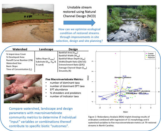
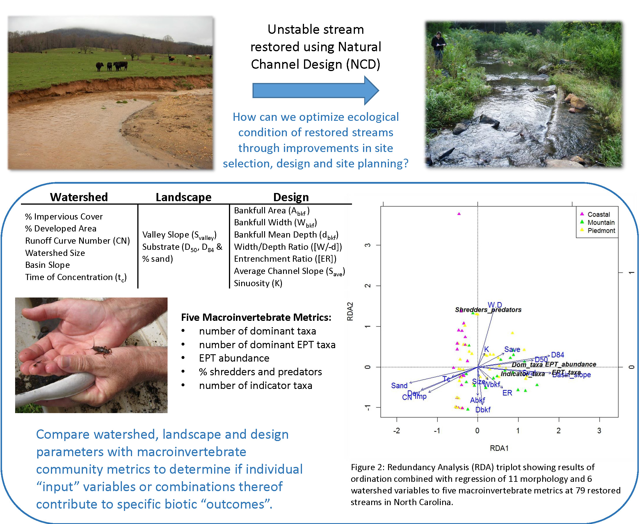
This study compares watershed, landscape, and design parameters (

Table 1. Watershed, landscape, and design variables hypothesized to influence stream restoration performance and biologic outcome.

Watershed	Landscape	Design
% Impervious Cover	Valley Slope (Svalley) Substrate (D50, D84, and % sand)	Bankfull Area (Abkf)
% Developed Area		Bankfull Width (Wbkf)
Runoff Curve Number (CN)		Bankfull Mean Depth (dbkf)
Watershed Size		Width/Depth Ratio ([W/d])
Basin Slope		Entrenchment Ratio ([ER])
Time of Concentration (tc)		Average Channel Slope (Save) Sinuosity (K)

) with macroinvertebrate community metrics to determine if individual “input” variables or combinations thereof contribute to specific biotic “outcomes”. From the site selection to the design process it would be beneficial to stream designers, conservationists, and environmental/mitigation policy makers to determine what factors (both controllable and non-controllable) affect the resulting biotic condition of the restored stream. This information may help to optimize performance of restoration efforts through improvements in site selection, stream design, and site planning.

2. Methods

2.1. Site Selection

Between 2006 and 2012, aquatic macroinvertebrates were sampled in 79 restored streams across the state as part of a North Carolina (NC) Clean Water Management Trust Fund (CWMTF) effort to assess restored streams [34]. The selection of streams assessed was a non-randomized sample based on available project documents and data, funding, and physical access. Only restored streams that applied NCD restoration practices [4], including modifications to channel and/or floodplain geometry and/or additions of rock and log structures, were included [19]. Based on a review of grant applications and project documents, many streams were targeted for restoration because of severe bank erosion and channel bed incision, which was considered detrimental to water quality and habitat. As such, stabilizing eroding stream banks and reconnecting the stream to a floodplain were the most commonly identified project goals. Improvement in biological habitat or integrity was also identified as a goal for a small subset of projects. The degree of restoration varied from enhancement (grading of floodplain benches and addition of rock and/or log structures) to complete channel relocation and/or reconfiguration of channel size and shape. The streams are located in a wide range of ecoregions, watershed conditions, bed material size classes, and valley types. Projects ranged in age from new construction to 10 years post-restoration. All sites were visited during March to October. Basic site information and design parameters were obtained for the restoration projects by contacting project designers and funding agencies. A map indicating the location of the 79 sites is provided in (Figure 1).

2.2. Macroinvertebrate Sampling

Aquatic macroinvertebrate samples were collected using a rapid method developed specifically for this project. The method was adapted from by the NC Division of Water Quality [35]. Samples were collected from at least one location within the restored stream channel. Each sample is a composite of macroinvertebrates collected by a kick net sample from a riffle area, a sweep net sample from bank habitats, a leaf pack sample, and visual inspections of stable substrate material. All specimens were identified to the lowest practical taxonomic level (i.e., genus and, in some cases, species) in the field by an experienced macroinvertebrate biologist, and all dominant taxa (two or more organisms) were recorded. Sampling results were used to calculate five macroinvertebrate metrics: number of dominant taxa (dominant taxa), number of dominant EPT taxa (EPT taxa), EPT abundance, percent shredders and predators, and number of indicator taxa (indicator taxa). EPT represents taxa from the “pollution sensitive” orders of Ephemeroptera (mayflies), Plecoptera (stoneflies), and Trichoptera (caddisflies). EPT taxa are widely used as indicators of environmental disturbances and urbanization [36] since they show a response to a wide array of pollutants over both long-term and short-term exposures; they are an indicator of flow persistence [37]; and are considered an appropriate richness measure for evaluating stream health [38]. The percent shredders and predators metric was selected as a surrogate for organic retention, which can be limiting in streams following restoration construction that includes extensive earthwork.

2.3. Substrate Sampling

A quantitative assessment of the dominant substrate material was also conducted as part of the assessment. Twenty-five substrate particles per riffle were collected from the baseflow wetted area along two riffles for a total of 50 particles collected from streams three meters wide or less, and 50 particles per riffle at two riffles for a total of 100 particles were collected for streams greater than three meters in width. Particles were collected while moving in a zigzag pattern across the entire riffle cover [17]. Individual particle measurements were made along the intermediate axis of each particle (or estimated for very small particles) following protocols developed by Wolman [39]. Particle sizes were recorded, and particle size distribution and cumulative frequency tallies were used to determine the D₅₀, D₈₄, and percent sand (<2 mm median diameter particle). The D₅₀ sediment size is the grain diameter at which 50% of the sediment sample is finer than, and the D₈₄ is the grain diameter at which 84% of the sediment sample is finer than. Substrate sampling was not conducted in sand bed streams.

2.4. Watershed Assessment

Watershed analysis was conducted for each stream using ArcGIS Desktop 10.0 [40]. Drainage boundaries for the downstream end of each restored stream reach were manually delineated referencing NC Department of Transportation county contour data [41], aerial photography, and hydraulic unit boundaries where applicable. Soil data from counties containing the target watersheds were obtained from the Natural Resources Conservation Services (NRCS) [42]. Watersheds were divided by hydrologic soil group (A, B, C, or D) according to soil type. Land use data were obtained from the US Geological Survey (USGS) National Land Cover Dataset [43]. Land cover data were reclassified to represent eight general land cover classes: water, developed, barren, forested, shrubland, herbaceous, cultivated, and wetlands according to the Multi-Resolution Land Characteristics Consortium (MRLC) 2001 landcover definitions [44]. The landcover data were then combined with the processed soils data to generate a composite runoff Curve Number (CN) for each watershed [45].

Impervious cover percentage was determined using the 2006 USGS National Land Cover Dataset (NLCD) Percent Developed Imperviousness [43] layer, which assigns an impervious cover percentage to each 30 m × 30 m pixel included in the dataset. A series of polygons that grouped pixels by impervious cover in 10 percent interval ranges (i.e., 1%–10%, 11%–20%, 21%–30%, etc.) was produced. Each polygon area was summarized to compute a composite impervious percentage for the total area of each individual watershed. Manual measurements were also taken in ArcGIS to determine the slope of the drainage basin and to estimate time of concentration ($t_c$) in minutes using the Kirpich Equation [46] for each restored reach.

$$t_c=\frac{{\left[\frac{L^3}{H}\right]}^{0.385}}{128}$$

(3)

where $L$ = hydraulic length or the longest flow path from the most remote point on the watershed ridge to the outlet of the watershed, measured in feet; and $H$ = height of the most remote point on the watershed ridge above the watershed outlet or the fall along the hydraulic length. The damping effect of inline water bodies, such as ponds and lakes, were ignored and hydraulic length was measured along the shortest distance across the water body. Basin slope was calculated by dividing basin height, $H,$ by hydraulic length, $L$. The Kirpich equation is generally limited to small rural watersheds of 0.8 square kilometers or less. This method is widely used in North Carolina for hydrologic analysis and was considered a reasonable method for making relative comparisons of general watershed size, morphology, and the associated flow path.

2.5. Statistical Analyses

Many of the landscape, watershed, design, and stream assessment variables lack independence. For example, channel dimension has been shown to relate to watershed size [12], as well as to percent impervious cover [28]. Cross-sectional area is a product of width and mean depth, and the [W/d] ratio is derived from the channel bankfull mean width and mean depth. Therefore, principal component analysis (PCA), a multivariate statistical technique designed to address multi-collinearity [47], was used for analyses. PCA was implemented on the scaled and centered matrix for various combinations of watershed, design, and landscape variables (Table 1) using R statistical software [48]. A sufficient number of principal components (PCs) were retained to explain a reasonable amount of the variability in the stream assessment variables (minimum of 75%). Afterwards, each macroinvertebrate metric was individually regressed on the retained subset of PCs. Varimax rotation of factors was used to increase loading coefficients for some variables in an effort to improve the interpretation of results from an ecological standpoint [49]. In addition, Redundancy Analysis (RDA), an extension of PCA that couples ordination and regression, was used to examine the relationships between the morphology and landscape variables and the five macroinvertebrate metrics. The “vegan” package in R statistical software [48] was used for the analysis. A triplot was prepared to show the results of exploring combinations of predictor variables (morphology and watershed) that best explain different combinations of response variables (macroinvertebrate metrics). Macroinvertebrate metric data were scaled and centered before performing the redundancy analysis to account for differences in units between the metrics.

Ridge regression using the “ridge” package in R statistical software [48] was used to develop models to predict macroinvertebrate metrics for the 79 restored streams. A ridge regression model was selected as it outperformed (resulted in the lowest prediction error using cross-validation) both principal component and least squares regression models in predicting EPT taxa numbers from rapid habitat assessment scores and watershed variables from this dataset [50]. Ridge regression stabilizes regression estimates in the presence of extreme multi-collinearity and shrinks the regression coefficients by imposing a penalty on their magnitude in order to minimize the residual sum of squares [51]. Various combinations of the landscape, watershed, and design variables in Table 1 were modeled for correlation to total number of dominant EPT taxa. The ridge models were used to calculate predicted EPT metric scores for the 79 restored streams. To evaluate predictive performance of the model, cross-validation using a leave-one-out method was performed. The ridge regression model was iteratively formulated 79 times by removing one single observation at a time from the data set. A predicted score for the missing observation and the associated prediction error were then calculated. The sum of the prediction errors equates to the overall prediction error or cross-validation score [52]. Predicted macroinvertebrate metrics from the cross-validation process were compared with field measured values to evaluate the fit of the model. Combinations of predictors were evaluated to determine if predictor weights were interpretable and would lend insight to site selection and design considerations for future restoration efforts.

3. Results

3.1. Correlation of Morphology Factors to Macroinvertebrates

A matrix of 11 individual design and landscape variables was standardized and PCA was applied in R statistical software [48] to generate PCs. Four PCs that explain 80.4% of the variance were retained. The scores from the four PCs were then used to perform multiple linear regression analysis in relation to five of the macroinvertebrate metric values. PC1 was found to have a statistically significant relationship with the total number of EPT taxa, EPT abundance, and total number of indicator taxa at the α = 0.05 level. PC2 had a statistically significant correlation with all macroinvertebrate metrics except percent shredders and predators, and PC3 only had a statistically significant correlation to the total number of abundant EPT taxa. PC4 was not significant. The resulting p-values that indicate significance for PC1, PC2, and PC3 are provided in

Table 2. p-values for all significant relationships resulting from multiple linear regression between macroinvertebrate metrics and morphology principal components (PCs).

PC#	No. Dominant Taxa	No. Dominant EPT Taxa	EPT Abundance	No. Indicator Taxa
PC1	–	0.00318	0.000576	0.031
PC2	2.04 × 10−7	2.7 × 10−8	9.52 × 10−7	1.6 × 10−6
PC3	–	0.04566	–	–

, and variable weights for the PCs are provided in

Table 3. PC weights for the first four PCs based on 11 morphology variables measured at 79 restored streams. Variables with higher weights are in bold.

Variable	PC1	PC2	PC3	PC4
Wbkf	−0.89	0.32	0.01	−0.24
Abkf	−0.83	0.41	−0.12	−0.18
dbkf	−0.76	0.49	−0.25	0.10
D50	−0.68	−0.54	−0.14	0.18
D84	−0.58	−0.73	−0.07	0.12
% sand	0.58	0.63	0.09	−0.25
Svalley	0.15	−0.80	0.07	−0.17
Save	0.10	−0.67	0.09	0.06
[W/d]	−0.35	−0.31	0.48	−0.63
K	0.23	−0.25	−0.54	−0.64
ER	0.24	−0.15	−0.82	−0.03

. PC1 is weighted most heavily by channel size and substrate. PC2 is weighted most heavily by channel size, substrate, and both channel and valley slope. Sinuosity and [W/d] ratio were heavily weighted positive variables for PC3 and PC4, while entrenchment ratio had a very large negative weight for PC3. These heavily weighted factors included in the top PCs appear to have a bearing on the macroinvertebrate metrics.

3.2. Accounting for Watershed Influence

To further explain variability in the relationships between site selection and design and macroinvertebrate metrics, six watershed factors (CN, percent impervious, percent developed, watershed size, basin slope, and time of concentration) were combined with the morphology variables, and PCA was again applied.

Table 4. Range, average, and median values for six watershed parameters.

Parameter	Range	Average	Median
Basin Slope	0.0019–0.1841	0.0333	0.0156
Tc (min.)	13.3–384	81.2	56.2
Watershed Size (sq. km.)	0.3–277	16.8	4.9
Curve Number	53–85.2	67.0	65.6
% Developed	0–99	36.9	16.5
% Impervious	0–52	11.0	1.6

provides the range, average, and median values for all six watershed parameters for the 79 restored streams. Five PCs were retained for assessment as they explain 80.9% of the variance. The scores from the retained PCs were used to perform multiple linear regression analysis in relation to the five macroinvertebrate metrics. The combination of six watershed factors with the morphology variables improved coefficients of determination when compared to individual macroinvertebrate metrics. Coefficients of determination based on 79 restored streams for each of the five macroinvertebrate metrics based on PCA of morphology variables alone and PCA of morphology combined with watershed factors are provided in

Table 5. Coefficients of determination resulting from linear regression of five macroinvertebrate metrics compared to four PCs resulting from site selection and morphology design variables (11 variables) and five PCs resulting from the morphology variables combined with six watershed factors. Total variance explained by the PCs is also reported. PCA refers to principal component analysis. EPT refers to Ephemeroptera (mayflies), Plecoptera (stoneflies), and Trichoptera (caddisflies).

Macroinvertebrate Metric/PCA Parameters	Linear Regression Approach
	PCA (Morph)	PCA (Morph + Watershed)
No. Dominant Taxa	0.46	0.58
No. Dominant EPT Taxa	0.51	0.66
EPT Abundance	0.46	0.59
% Shredders and Predators	0.15	0.20
No. Indicator Taxa	0.42	0.57
No. of Variables	11	17
Total No. of PC‘s	4	5
% Variability Explained	80.4%	80.9%

.

RDA analysis was used to further explore relationships between the macroinvertebrate metrics and the predictor variables (morphology and watershed). Scores from RDA analysis were used to prepare a triplot that simultaneously displays stream scores (based on RDA axes one and two, which explain 66.6% of the variance) as points, macroinvertebrate metric scores as points, and the watershed and morphology variables as arrows (Figure 2). The triplot displays correlation information amongst variables through the angles between the points and arrows. Small angles between two variable arrows imply high positive correlations between these variables, and variable arrows pointing the same direction or species points in the same location reveal intercorrelations of these variables. Arrows pointing in opposite directions are negatively correlated. The triplot reveals redundancies in channel size, slope, and watershed variables. EPT abundance and taxa are closely grouped and dominant taxa and indicator taxa are also closely located to EPT. These four metrics show a strong positive association with slope (basin and valley) and substrate particle size (D₅₀ and D₈₄), and a negative correlation with watershed development variables (percent developed, percent impervious, and CN) and the percent of sand. However, shredders and predators is located separately from the other four metrics and is positively correlated with width-to-depth ratio, [W/d]. The tri-plot is color-coded by physiographic region and reveals a separation between coastal plain and mountain sites. Coastal plain includes both the Middle Atlantic Coastal and Southeastern Plain regions shown in Figure 1. In contrast, the Piedmont streams are more widely dispersed. The plot also displays an outlier coastal plain stream where only amphipods were found, producing a 100% shredders and predators metric score.

3.3. Predicting EPT Taxa from Design and Site Selection

In an effort to further interpret the relationship among site selection, design, and biologic outcomes, ridge regression was used to develop a linear model of the morphology and watershed variables that would reduce the prediction error for Dominant EPT Taxa for the 79 restored streams. Dominant EPT taxa was selected for regression analysis since they are widely used as indicators of environmental disturbances [53] and considered an appropriate richness measure for evaluating stream health [38]. Using morphology variables alone resulted in reasonable prediction of dominant EPT taxa for the 79 restored streams (R² = 0.62). Prediction values did not cover the range of the measured values, and the mean of predicted values was higher than the measured mean. The resulting ridge regression model for predicting dominant EPT taxa using the morphologic factors is:

EPT = I + β₀× x₁ + β₁× x₂ + β₂× x₃ +…+ β₁₀× x₁₁

(4)

where EPT = expected total number of dominant EPT taxa. I = the Y intercept, which is 4.44, and the beta values for each of the 11 variables (x’s) included in the ridge regression model are reported in

Table 6. Coefficients or weights for each morphology factor (design and landscape) resulting from ridge regression. Variables with higher weights are in bold.

Positive		Negative
D84	1.68	% Sand	−1.48
ER	1.22	Abkf	−0.80
Svalley	1.10	D50	−0.39
dbkf	0.78	Save	−0.35
Wbkf	0.38	K	−0.22
[W/d]	0.01	–	–

. Values for betas are grouped by positive and negative weights. Variables that carry the heaviest positive weight (largest beta) and thus have the greatest influence for predicting dominant EPT taxa values included D₈₄, ER, S_valley, and d_bkf. Variables having the most significant negative weight included percent sand and A_bkf. Therefore as these factors increase, the number of predicted dominant EPT taxa decreases. The positive influence of bankfull mean depth countered by the negative influence of bankfull channel area makes interpretation of this model difficult.

The ridge model was then repeated using the 11 morphology variables combined with six watershed factors. The watershed variables improved prediction of EPT taxa over morphology variables alone (R² = 0.82). The range of predicted values was similar, however, the predicted mean value was lower, bringing it closer to the measured mean value. The Y intercept for the model remained at 4.44, and the beta values for each of the 17 variables (morphology and watershed) included in the ridge regression model are reported in

Table 7. Coefficients or weights for each morphology and watershed factor resulting from ridge regression. Variables with higher weights are in bold.

Positive		Negative
Svalley	1.14	% Developed	−1.44
dbkf	1.00	% Sand	−1.28
ER	0.91	CN	−1.06
Basin slope	0.86	Size	−1.02
D84	0.62	Save	−0.49
Wbkf	0.50	K	−0.48
% Impervious	0.47	D50	−0.18
tc	0.17	Abkf	−0.16
–	–	[W/d]	−0.12

. Variables that have heavier positive weight (largest beta) and thus have greater influence for predicting dominant EPT taxa values included channel size (d_bkf, W_bkf), floodplain width (ER), slope (S_valley, basin slope), level of development (percent impervious), and substrate (D₈₄). Variables having the most significant negative weight included percent developed, CN, watershed size, S_ave, percent sand, and sinuosity (K). Results were somewhat difficult to interpret as similar variables have both positive and negative weights in the model. For example, the negative influence of percent developed and CN on EPT taxa, which were expected, are countered by the positive influence of percent impervious. Similarly, basin slope and valley slope contribute positively to the number of dominant EPT taxa, but this is countered by a negative influence of average channel slope. Also, the positive influence of bankfull mean depth and width are countered by a minor negative influence of bankfull channel area. This example is less pronounced than the first two since A_bkf has a fairly low negative weight. These statistically anomalous variable conflicts limit the ability to interpret the model in a way that provides insight for future project selection and design. In an effort to improve interpretation of the ridge model, variable elimination based on correlation of variables was pursued.

A color-coded correlation diagram was produced using the “corrgram” package in R statistical software [48] (Figure 3). The diagram indicates the strongest positive correlations between A_bkf and watershed size, t_c, W_bkf and d_bkf; between CN and percent impervious and percent developed; and between D₈₄ and D₅₀ particle size classes. The highest negative correlation is between percent sand and the D₈₄ and D₅₀ particle size classes. Considering the correlation diagram and the RDA triplot of the first two RDA axes for the watershed and morphology variables (Figure 2), where redundant variables can be identified by vectors aligned along the same axis, eight variables, including A_bkf, d_bkf, S_ave, percent impervious, percent developed, percent sand, D₈₄, and watershed size, were eliminated. The ridge model was then rerun with the nine variables retained. Cross-validation using a leave-one-out approach produced predicted EPT taxa values with a comparable range and mean to the observed values (Figure 4). Linear comparison of the ridge regression model scores to the measured values resulted in a significant decrease in the coefficient of determination (R² = 0.67). The coefficient did represent a notable improvement over the ridge model using the morphology variables alone (R² = 0.62). The Y intercept for the model again remained at 4.44, and the beta values for each of the nine variables (morphology and watershed) included in the ridge regression model are reported in

Table 8. Coefficients or weights for each morphology and watershed factor resulting from ridge regression following variable elimination.

Positive		Negative
Basin Slope	1.66	CN	−1.42
ER	1.02	K	−0.46
D50	0.81	[W/d]	−0.42
Svalley	0.74	tc	−0.05
Wbkf	0.74	–	–

. Variables that carry the heaviest positive weight (largest beta) and thus have the greatest influence for predicting dominant EPT taxa values included basin slope, floodplain width (ER), substrate (D₅₀), slope (S_valley), and channel size (W_bkf). Variables having the most significant negative weight included CN, sinuosity (K), and [W/d]. Even though the ridge model that was produced following variable elimination exhibits reduced prediction accuracy, the results were more easily interpreted from a practical standpoint. From the coefficient weights in Table 8 one can surmise that larger (wider) streams in steeper valleys with larger substrate and undeveloped watersheds will have higher numbers of dominant EPT taxa. This result is obvious, given the fact that low EPT taxa numbers were found in the lower gradient, sand-bed dominated Coastal Plain streams compared to the Piedmont and Mountain streams (Figure 5), and lower EPT taxa numbers were also found in urban streams (≥10% impervious) when compared to rural streams (<10% impervious) (Figure 6). However, it appears that larger accessible floodplain widths (high ER values) correlate with higher EPT taxa values and that in contrast, high width-to-depth ratios, [W/d], and high levels of sinuosity, K, correlate with lower EPT taxa numbers, which are not obvious conclusions resulting from urbanization or physiographic region factors.

4. Discussion

Principal component regression analysis of 79 restored streams indicated that 11 morphology related stream design and landscape variables were found to be significantly related to four macroinvertebrate metrics, including number of abundant taxa, number of indicator taxa, and number and abundance of EPT taxa. The linear regression revealed that the morphology PCs did not explain a significant portion of the variability in the macroinvertebrate metrics. Further, PCA of a combined matrix of watershed conditions with morphology variables improved correlation when the resulting PCs were linearly regressed in relation to the macroinvertebrate metrics. These results suggest that site selection, including watershed condition, and design procedures and decisions made by the project managers and designers have an influence on the biological outcome of the stream restoration project. Further, this study confirms the influence of watershed condition on macroinvertebrate community metrics that is previously well documented [32,36,54].

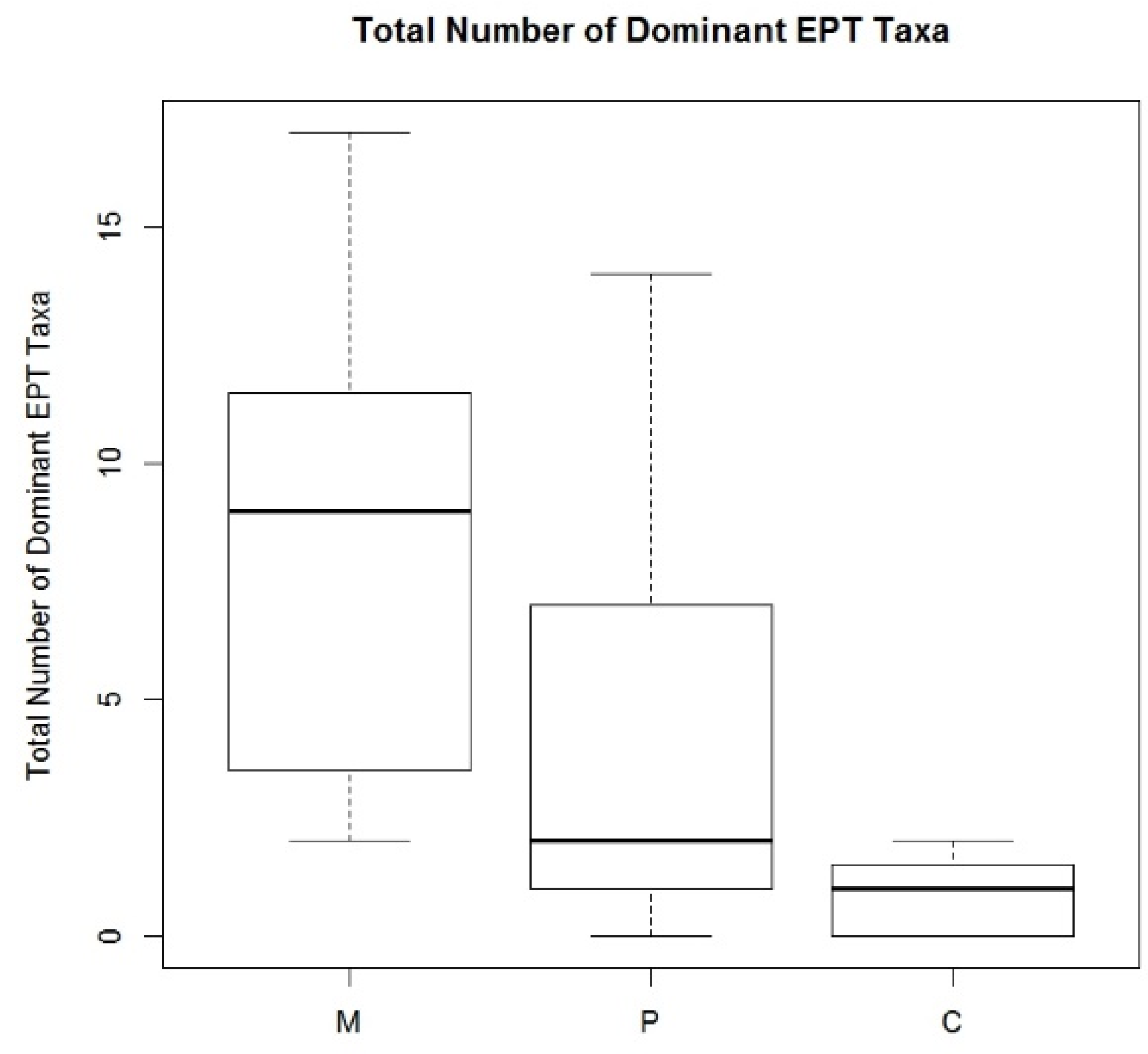
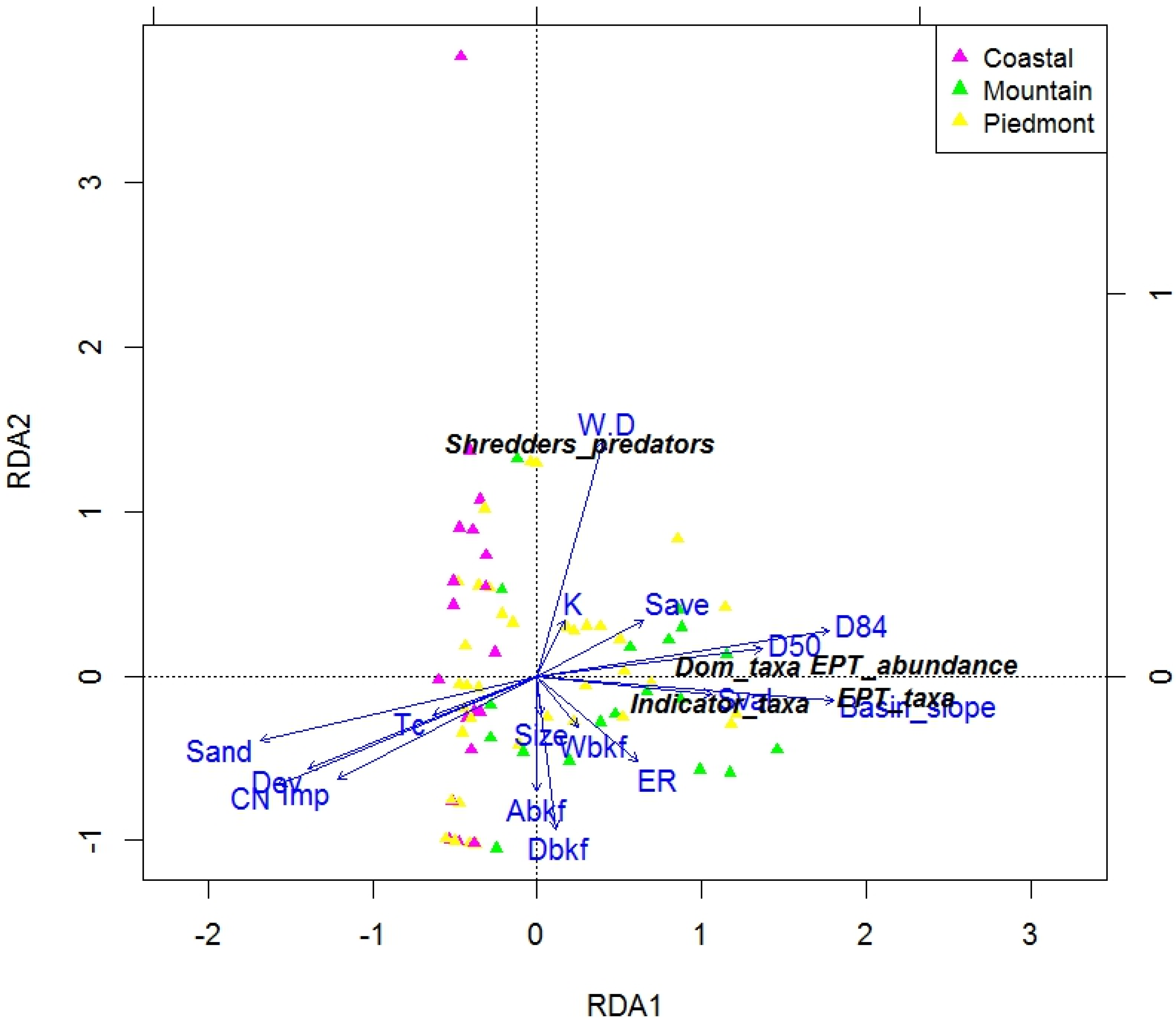
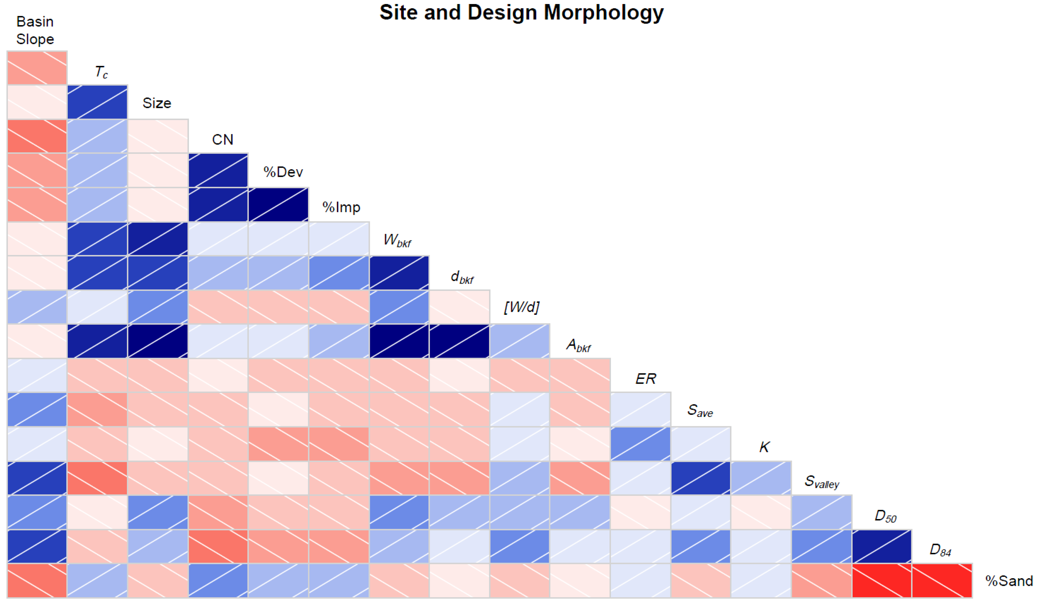
Ridge regression of 11 morphology variables was successfully used to predict the number of dominant EPT taxa compared to measured values from field sampling of the 79 restored streams (R² = 0.62). The ridge model was improved by adding six watershed variables (R² = 0.82). However, the interpretation of the ridge regression model relative to site selection and design was difficult due to both negative and positive weighting of variables with correlation. Therefore, variable reduction using a correlation matrix and interpretation of an RDA triplot resulted in the selection of nine variables to retain for ridge regression. Variables retained included bankfull channel mean width, width-to-depth ratio, entrenchment ratio, sinuosity, valley slope, basin slope, median substrate particle size, time of concentration, and runoff curve number. 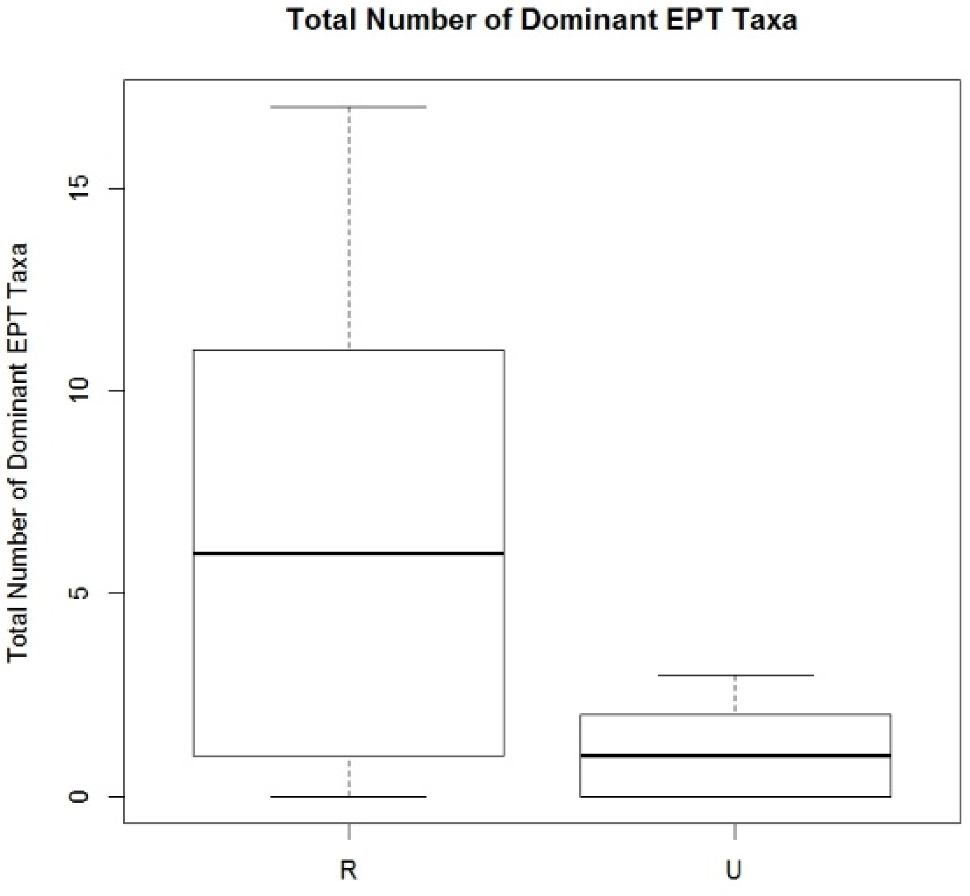The reduced model improved interpretation of the results while also providing a reasonable prediction of EPT taxa (R² = 0.67). The model indicated that larger (wider) streams in steeper valleys with larger substrate and undeveloped watersheds will have higher numbers of dominant EPT taxa. This result was expected given the extremely low EPT taxa numbers that were found in lower gradient, sand-bed dominated Coastal Plain streams and in urban streams (percent impervious ≥ 10). The increase in channel size (e.g., width) positively affecting macroinvertebrate community metrics has been seen in several regions around the world [55,56]. Further, the model results reflect the disparity in EPT taxa and other macroinvertebrates between regions and watershed conditions in North Carolina. These results support findings of no difference in macroinvetebrate communities between urban degraded and restored channels in the Piedmont region of North Carolina [57]. Rather, macroinvertebrate metrics were best predicted by channel habitat complexity and watershed impervious cover.

The reduced ridge regression model also indicates that larger accessible floodplain widths (higher ER values) correlate with higher EPT taxa values, and, in contrast, high width-to-depth ratios, [W/d], and high levels of sinuosity, K, correlate with lower EPT taxa numbers. Therefore, expanding floodplain area should be a focus of restoration projects, especially when project goals include improving macroinvertebrate diversity. Increasing floodplain connectivity and width is also likely to enhance nutrient removal [58,59,60,61,62,63]. In contrast to entrenchment ratio, increasing sinuosity may not be a primary concern for macroinvertebrate community improvement. Many streams in need of restoration and enhancement occur in restricted corridors where increasing sinuosity is difficult. Doyle et al. [64] found a slightly higher, yet significant, increase in sinuosity among streams built for mitigation purposes versus those for non-mitigation purposes in North Carolina and suggested that this was a result of restoration designers striving to increase the length of the restored stream to maximize mitigation credits, and thus economic benefits, of the project. This study indicates that increasing the floodplain width will afford greater improvements in macroinvertebrate community over sinuosity. However, increasing sinuosity may have a positive effect on nutrient removal similar to increasing floodplain area and access. This may be true especially for streams of less than 10 meters in width, as these channels frequently remove as much as 50% of the nitrogen produced by their watershed, with uptake and removal occurring on submerged sediments and biofilm [65]. For example, restored sections of Wilson Creek in Kentucky showed improved nutrient uptake and reduced flow velocity when compared to the unrestored reaches [60]. Therefore increasing sinuosity combined with improving frequency of floodplain access would be appropriate targets for removing nitrogen.

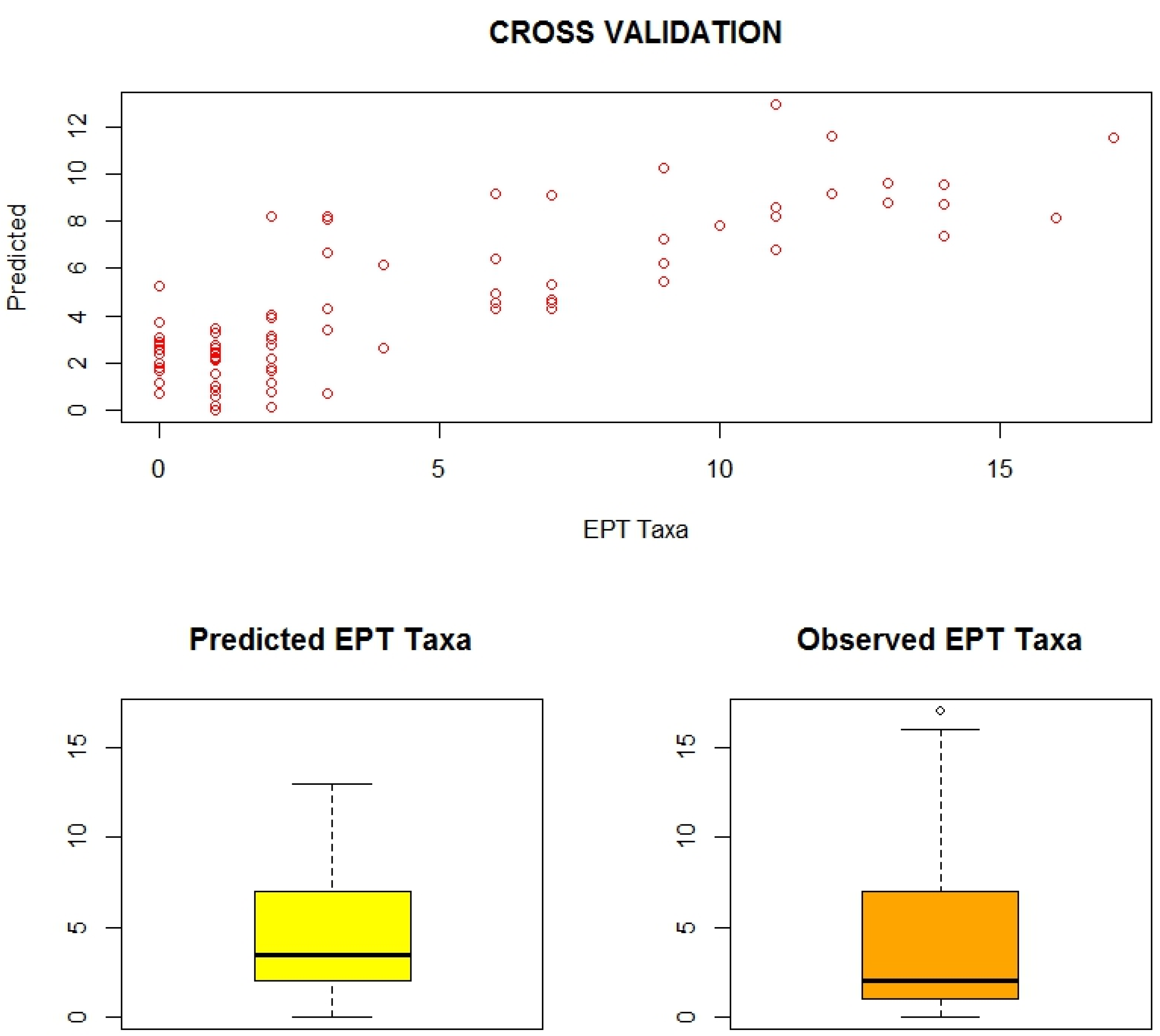
Larger width-to-depth ratio negatively influencing EPT taxa numbers may indicate that wide-shallow streams have an influence on the macroinvertebrate community. However, it should be noted that high EPT abundance was primarily associated with medium sized watersheds of greater than 2.6 to less than 26 square kilometers. Width-to-depth ratio interacts with many other geomorphic parameters (pool depth, velocity, shear stress, substrate size, etc.) making conclusions about this result difficult. The PCR and ridge regression models developed to predict EPT taxa reflect the range of conditions of the 79 restored streams sampled by this study in North Carolina. Further, cross-validation revealed that the ridge model is likely be a good predictor of EPT taxa numbers in other restored streams located in the state. However, these regression models should not be used to predict EPT taxa in other states or regions of the country where the range of variability and the importance of each predictor are likely to differ.

Given the lack of EPT taxa expected to occur in coastal and urban settings regardless of restoration activities, other biological and ecosystem metrics should be considered for evaluating project need, site selection, design, and performance of urban and coastal stream restoration efforts. Strongly considering physical form or morphology of a stream restoration project as a logical objective to assess in addition to habitat and biology, the Ohio Department of Environment and Natural Resources evaluated 51 restored streams using assessment parameters that addressed a variety of characteristics that were measurable, products of design, and deemed necessary for ecological function [66]. As a result, stream power, channel size, flood frequency, floodplain extent, floodplain connectivity, and sinuosity at the restored streams were compared to benchmarks developed from the literature, modeling, and/or field data collected from non-restored streams in Ohio. Woolsey et al. [7] identify 49 indicators designed to assess 13 potential objectives including social, environmental, and economic factors likely relevant to stream restoration. More recently, Starr et al. [67] developed a function-based assessment tool for stream restoration that applies a number of existing and new measurement methods and performance standards for use in assessing project need and quantifying functional uplift of restoration efforts. This tool strongly emphasizes watershed hydrology, channel and floodplain hydraulics, geomorphology, and physicochemical parameters as controlling factors in the ultimate biological condition of the restored stream. If the relationships between these factors are not considered, then unrealistic and unachievable goals and objectives and subsequent associated target success metrics will be established for projects.

References

1. Rosgen, D.L. A classification of natural rivers. CATENA 1994, 22, 169–199. [Google Scholar] [CrossRef]
2. Rosgen, D.L. Applied River Morphology; Wildland Hydrology: Pagosa Springs, CO, USA, 1996. [Google Scholar]
3. Rosgen, D.L. A geomorphological approach to restoration of incised rivers. In Proceedings of the Conference on Management of Landscapes Disturbed by Channel Incision, Oxford, MS, USA, 19 May 1997.
4. Hey, R.D. Fluvial geomorphological methodology for natural stable channel design. J. Am. Water Resour. Assoc. 2006, 42, 357–374. [Google Scholar] [CrossRef]
5. Restoration cowboy goes against the flow. High Country News. Available online: http://www.hcn.org/issues/262/14362 (accessed on 14 April 2016).
6. Bernhardt, E.S.; Sudduth, E.B.; Palmer, M.A.; Allan, J.D.; Meyer, J.L.; Alexander, G.; Follastad-Shah, J.; Hassett, B.; Jenkinson, R.; Lave, R.; et al. Restoring rivers one reach at a time: Results from a survey of U.S. River restoration practitioners. Restor. Ecol. 2007, 15, 482–493. [Google Scholar] [CrossRef]
7. Woolsey, S.; Capelli, F.; Gonser, T.O.M.; Hoehn, E.; Hostmann, M.; Junker, B.; Paetzold, A.; Roulier, C.; Schweizer, S.; Tiegs, S.D.; et al. A strategy to assess river restoration success. Freshw. Biol. 2007, 52, 752–769. [Google Scholar] [CrossRef]
8. Davis, W. Baselevel, grade and peneplain. J. Geol. 1902, 10, 77–111. [Google Scholar] [CrossRef]
9. Leopold, L.B.; Wolman, M.G.; Miller, J.P. Fluvial Processes in Geomorphology; Courier Corporation: Mineola, NY, USA, 2012. [Google Scholar]
10. Strahler, A.N. Quantitative analysis of watershed geomorphology. Civ. Eng. 1957, 101, 1258–1262. [Google Scholar] [CrossRef]
11. Hey, R.D. Stable river morphology. In Applied Fluvial Geomorphology for River Engineering and Management; Thorne, C.R., Hey, R.D., Newson, M.D., Eds.; John Wiley & Sons Ltd: Hoboken, NJ, USA, 1997; pp. 223–236. [Google Scholar]
12. Leopold, L.B. A View of the River; Harvard University Press: Cambridge, MA, USA, 1994. [Google Scholar]
13. Dunne, T.; Leopold, L.B. Water in Environmental Planning; W.H. Freeman Co.: New York, NY, USA, 1978. [Google Scholar]
14. Giller, P.S. River restoration: Seeking ecological standards. Editor’s introduction. J. Appl. Ecol. 2005, 42, 201–207. [Google Scholar] [CrossRef]
15. Clewell, A.; Rieger, J.P. What practitioners need from restoration ecologists. Restor. Ecol. 1997, 5, 350–354. [Google Scholar] [CrossRef]
16. Rosgen, D.L. The Reference Reach: A Blueprint for Natural Channel Design; Draft Presented at ASCE Conference on River Restoration in Denver, CO, USA, 1998.
17. Doll, B.A.; Grabow, G.L.; Hall, K.R.; Halley, J.; Harman, W.A.; Jennings, G.D.; Wise, D.E. Stream Restoration: A Natural Channel Design Handbook; North Carolina Stream Restoration Institute, NC State University: Raleigh, NC, USA, 2003. [Google Scholar]
18. Wildland, H.I. Level IV: River Restoration and Natural Channel Design; Wildlands Hydrology: Silverthorne, CO, USA, 1999. [Google Scholar]
19. USDA. Rosgen Geomorphic Channel Design. In Stream Restoration Design National Engineering Handbook Part; USDA: Washington, DC, USA, 2007. [Google Scholar]
20. Shields, A. Application of Similarity Principles and Turbulence Research to the Bed Load Movement; Hydrodynamics Laboratory: Pasadena, CA, USA, 1936. [Google Scholar]
21. Andrews, E.D. Entrainment of gravel from naturally sorted riverbed material. Geol. Soc. Am. Bull. 1983, 94, 1225–1231. [Google Scholar] [CrossRef]
22. Athansakes, G.; Rosgen, D.L. Application of the flowsed and powersed models in river stability, bridge design and river restoration. In Proceedings of the 2nd Joint Federal Interagency Conference, Las Vegas, NV, USA, 27 June–1 July 2010.
23. Bernhardt, E.S.; Palmer, M.A. Restoring streams in an urbanizing world. Freshw. Biol. 2007, 52, 738–751. [Google Scholar] [CrossRef]
24. Schueler, T.R. The Importance of Imperviousness; Protection, C.F.W., Ed.; Center for Watershed Protection: Ellicott City, ML, USA, 1994; pp. 100–111. [Google Scholar]
25. Booth, D.B.; Jackson, C.R. Urbanization of aquatic systems: Degradation thresholds, stormwater detection, and the limits of mitigation. J. Am. Water Resour. Assoc. 1997, 33, 1077–1090. [Google Scholar] [CrossRef]
26. Hammer, T.R. Impacts of Urbanization on Peak Streamflow; Regional Science Research Institute: Philadelphia, PA, USA, 1973. [Google Scholar]
27. Hammer, T.R. Stream Channel Enlargement Due to Urbanization; Regional Science Research Institute: Philadelphia, PA, USA, 1972. [Google Scholar]
28. Doll, B.A.; Wise-Frederick, D.E.; Buckner, C.M.; Wilkerson, S.D.; Harman, W.A.; Smith, R.E.; Spooner, J. Hydraulic geometry relationships for urban streams throughout the piedmont of north Carolina. J. Am. Water Resour. Assoc. 2002, 38, 641–651. [Google Scholar] [CrossRef]
29. Shields, F., Jr.; Knight, S.; Cooper, C. Effects of channel incision on base flow stream habitats and fishes. Environ. Manag. 1994, 18, 43–57. [Google Scholar] [CrossRef]
30. Shields, F.D.; Lizotte, R.E.; Knight, S.S.; Cooper, C.M.; Wilcox, D. The stream channel incision syndrome and water quality. Ecol. Eng. 2010, 36, 78–90. [Google Scholar] [CrossRef]
31. Shields, F.; Knight, S.; Cooper, C. Rehabilitation of aquatic habitats in warmwater streams damaged by channel incision in Mississippi. Hydrobiologia 1998, 382, 63–86. [Google Scholar] [CrossRef]
32. Deacon, J.R.; Soule, S.A.; Smith, T.E. Effects of Urbanization on Stream Quality at Selected Sites in the Seacoast Region in New Hampshire, 2001–2003; US Department of the Interior, US Geological Survey: Reston, VA, USA, 2005.
33. Booth, D.B.; Karr, J.R.; Schauman, S.; Konrad, C.P.; Morley, S.A.; Larson, M.G.; Burges, S.J. Reviving urban streams: Land use, hydrology, biology, and human behavior. J. Am. Water Resour. Assoc. 2004, 40, 1351–1364. [Google Scholar] [CrossRef]
34. NCSU Water Quality Group. Stream Restoration Evaluation Assessment Form; NCSU: Raleigh, NC, USA, 2006; p. 37. [Google Scholar]
35. Standard Operating Procedures for Biological Monitoring; Division of Water Quality; NCDENR: Raleigh, NC, USA, 2006; p. 52.
36. Purcell, A.H.; Friedrich, C.; Resh, V.H. An assessment of a small urban stream restoration project in northern California. Restor. Ecol. 2002, 10, 685–694. [Google Scholar] [CrossRef]
37. Feminella, J.W. Comparison of benthic macroinvertebrate assemblages in small streams along a gradient of flow permanence. J. N. Am. Benthol. Soc. 1996, 15, 651–669. [Google Scholar] [CrossRef]
38. Barbour, M.T.; Gerritsen, J.; Snyder, B.; Stribling, J. Rapid Bioassessment Protocols for Use in Streams and Wadeable Rivers; USEPA: Washington, DC, USA, 1999. [Google Scholar]
39. Wolman, M.G. A method of sampling coarse river-bed material. EOS Trans. Am. Geophys. Union 1954, 35, 951–956. [Google Scholar] [CrossRef]
40. Arcgis Desktop: Release 10; Environmental Systems Research Institute: Redlands, CA, USA, 2011.
41. Contour and Elevation Data; NC Department of Transportation: Raleigh, NC, USA, 2007.
42. Soil Survey Geographic (SSURGO) Database for North Carolina and Virginia; USDA-NRCS: Lincoln, NE, USA, 2012.
43. Fry, J.A.; Xian, G.; Jin, S.; Dewitz, J.A.; Homer, C.G.; Limin, Y.; Barnes, C.A.; Herold, N.D.; Wickham, J.D. Completion of the 2006 national land cover database for the conterminous united states. Photogramm. Eng. Remote Sens. 2011, 77, 858–864. [Google Scholar]
44. NLCD 2001 Land Cover Class Definitions, Multi-Resolution Land Characteristics Consortium (MRLC); USEPA: Washington, DC, USA, 2007.
45. Hydrologic Soil-Cover Complexes, Chapter 9, National Engineering Handbook: Part 630-Hydrology; USDA Soil Conservation Service: Washington, DC, USA, 2004; p. 20.
46. Bureau of Reclamation. Design of Small Dams; USGPO: Washington, DC, USA, 1974. [Google Scholar]
47. Jolliffe, I. Principal Component Analysis; Wiley: Hoboken, NJ, USA, 2002. [Google Scholar]
48. R Core Team. A Language and Environment for Statistical Computing; R Foundation For Statistical Computing: Vienna, Austria, 2012. [Google Scholar]
49. Mahmood, R.; Messer, J.J.; Nemanich, F.J.; Liff, C.I.; George, D.B. A Multivariate Water Quality Index for Use in Management of a Wildland Watershed; UWRL: Logan, UT, USA, 1982. [Google Scholar]
50. Doll, B.A.; Jennings, G.D.; Spooner, J.; Penrose, D.L.; Usset, J.L. Evaluating the eco-geomorphological condition of restored streams using visual assessment and macroinvertebrate metrics. J. Am. Water Resour. Assoc. 2015, 51, 68–83. [Google Scholar] [CrossRef]
51. Hastie, T.; Tibshirani, R.; Friedman, J.; Franklin, J. The elements of statistical learning: Data mining, inference and prediction. Math. Intell. 2005, 27, 83–85. [Google Scholar]
52. Picard, R.R.; Cook, R.D. Cross-validation of regression models. J. Am. Stat. Assoc. 1984, 79, 575–583. [Google Scholar] [CrossRef]
53. Griffith, M.B.; Hill, B.H.; McCormick, F.H.; Kaufmann, P.R.; Herlihy, A.T.; Selle, A.R. Comparative application of indices of biotic integrity based on periphyton, macroinvertebrates, and fish to southern rocky mountain streams. Ecol. Indic. 2005, 5, 117–136. [Google Scholar] [CrossRef]
54. Moore, A.A.; Palmer, M.A. Invertebrate biodiversity in agricultural and urban headwater streams: Implications for conservation and management. Ecol. Appl. 2005, 15, 1169–1177. [Google Scholar] [CrossRef]
55. Heino, J.; Muotka, T.; Paavola, R. Determinants of macroinvertebrate diversity in headwater streams: Regional and local influences. J. Anim. Ecol. 2003, 72, 425–434. [Google Scholar] [CrossRef]
56. Paller, M.H.; Specht, W.L.; Dyer, S.A. Effects of stream size on taxa richness and other commonly used benthic bioassessment metrics. Hydrobiologia 2006, 568, 309–316. [Google Scholar] [CrossRef]
57. Violin, C.R.; Cada, P.; Sudduth, E.B.; Hassett, B.A.; Penrose, D.L.; Bernhardt, E.S. Effects of urbanization and urban stream restoration on the physical and biological structure of stream ecosystems. Ecol. Appl. 2011, 21, 1932–1949. [Google Scholar] [CrossRef] [PubMed]
58. Fennessy, M.; Cronk, J. The effectiveness and restoration potential of riparian ecotones for the management of nonpoint source pollution, particularly nitrate. Crit. Rev. Environ. Sci. Technol. 1997, 27, 285–317. [Google Scholar] [CrossRef]
59. Fischenich, C.; Morrow, J.V., Jr. Reconnection of Floodplains with Incised Channels; DTIC Document; US Army Corps of Engineers: Vicksburg, MS, USA, 2000.
60. Bukaveckas, P.A. Effects of channel restoration on water velocity, transient storage, and nutrient uptake in a channelized stream. Environ. Sci. Technol. 2007, 41, 1570–1576. [Google Scholar] [CrossRef] [PubMed]
61. Craig, L.S.; Palmer, M.A.; Richardson, D.C.; Filoso, S.; Bernhardt, E.S.; Bledsoe, B.P.; Doyle, M.W.; Groffman, P.M.; Hassett, B.A.; Kaushal, S.S. Stream restoration strategies for reducing river nitrogen loads. Front. Ecol. Environ. 2008, 6, 529–538. [Google Scholar] [CrossRef]
62. Kaushal, S.S.; Groffman, P.M.; Mayer, P.M.; Striz, E.; Gold, A.J. Effects of stream restoration on denitrification in an urbanizing watershed. Ecol. Appl. 2008, 18, 789–804. [Google Scholar] [CrossRef] [PubMed]
63. Filoso, S.; Palmer, M.A. Assessing stream restoration effectiveness at reducing nitrogen export to downstream waters. Ecol. Appl. 2011, 21, 1989–2006. [Google Scholar] [CrossRef] [PubMed]
64. Doyle, M.W.; Singh, J.; Lave, R.; Robertson, M.M. The morphology of streams restored for market and nonmarket purposes: Insights from a mixed natural-social science approach. Water Resour. Res. 2015, 51, 5603–5622. [Google Scholar] [CrossRef]
65. Peterson, B.J.; Wollheim, W.M.; Mulholland, P.J.; Webster, J.R.; Meyer, J.L.; Tank, J.L.; Martí, E.; Bowden, W.B.; Valett, H.M.; Hershey, A.E. Control of nitrogen export from watersheds by headwater streams. Science 2001, 292, 86–90. [Google Scholar] [CrossRef] [PubMed]
66. Mecklenburg, D.; Fay, L.A. A Functional Assessment of Stream Restoration in Ohio; Ohio Department of Natural Resources, Division of Soil and Water Resources: Chillicothe, OH, USA, 2011. [Google Scholar]
67. Starr, R.; Harman, W.A.; Davis, S. Final Draft Function-Based Rapid Stream Assessment Methodology Assessment Methodology; Habitat Restoration Division, U.S. Fish and Wildlife Service: Annapolis, MD, USA, 2015. [Google Scholar]
Figure 1. Location of restored streams with design and morphology data.
Water 08 00151 g001
Figure 2. Redundancy Analysis (RDA) triplot showing results of ordination combined with regression of 11 morphology and six watershed variables to five macroinvertebrate metrics at 79 streams.
Water 08 00151 g002
Figure 3. Correlation matrix diagram for 11 landscape and design morphology and six watershed variables. Blue indicates positive and red indicates negative correlation. Darker shades represent higher levels of correlation between variables.
Water 08 00151 g003
Figure 4. Scatterplot and box plot comparison of predicted number of dominant EPT Taxa resulting from cross-validation of ridge regression model (Predicted EPT Taxa) of six morphology combined with three watershed variables after variable elimination compared with measured (Observed EPT Taxa) number of dominant EPT taxa values for 79 restored streams. Predicted values have been truncated at zero.
Water 08 00151 g004
Figure 5. Total Number of Dominant EPT Taxa for mountain (M), Piedmont (P), and coastal plain (C) streams (n = 79).
Water 08 00151 g005
Figure 6. Total Number of Dominant EPT Taxa for urban (% Impervious ≥ 10) vs. rural (% Impervious < 10) Streams (n = 79).
Water 08 00151 g006