Monthly Rainfall Erosivity: Conversion Factors for Different Time Resolutions and Regional Assessments

Abstract

As a follow up and an advancement of the recently published Rainfall Erosivity Database at European Scale (REDES) and the respective mean annual R-factor map, the monthly aspect of rainfall erosivity has been added to REDES. Rainfall erosivity is crucial to be considered at a monthly resolution, for the optimization of land management (seasonal variation of vegetation cover and agricultural support practices) as well as natural hazard protection (landslides and flood prediction). We expanded REDES by 140 rainfall stations, thus covering areas where monthly R-factor values were missing (Slovakia, Poland) or former data density was not satisfactory (Austria, France, and Spain). The different time resolutions (from 5 to 60 min) of high temporal data require a conversion of monthly R-factor based on a pool of stations with available data at all time resolutions. Because the conversion factors show smaller monthly variability in winter (January: 1.54) than in summer (August: 2.13), applying conversion factors on a monthly basis is suggested. The estimated monthly conversion factors allow transferring the R-factor to the desired time resolution at a European scale. The June to September period contributes to 53% of the annual rainfall erosivity in Europe, with different spatial and temporal patterns depending on the region. The study also investigated the heterogeneous seasonal patterns in different regions of Europe: on average, the Northern and Central European countries exhibit the largest R-factor values in summer, while the Southern European countries do so from October to January. In almost all countries (excluding Ireland, United Kingdom and North France), the seasonal variability of rainfall erosivity is high. Very few areas (mainly located in Spain and France) show the largest from February to April. The average monthly erosivity density is very large in August (1.67) and July (1.63), while very small in January and February (0.37). This study addresses the need to develop monthly calibration factors for seasonal estimation of rainfall erosivity and presents the spatial patterns of monthly rainfall erosivity in European Union and Switzerland. Moreover, the study presents the regions and seasons under threat of rainfall erosivity.

1. Introduction

Soil erosion by water is usually takes place in non-flat areas, when rainfall (and consequently surface runoff) falls on soils poorly covered with vegetation and without protective measures [1]. In Europe, soil loss by water erosion is mostly modeled using the Revised Universal Soil Loss Equation (RUSLE) [2]. RUSLE takes into consideration 6 factors: rainfall erosivity, soil erodibility, slope steepness and length, cover-management, and support practices. These factors are characterized by large spatial variability across the European Union, resulting in very heterogeneous spatial patterns of soil loss. Among the six factors, rainfall erosivity and cover-management have a high temporal variability during the different months of the year. Thus, data on rainfall erosivity in combination with vegetation cover and support management practices can facilitate useful assessments of soil erosion at local/regional scales to large scales. Further, the intra-annual variation in rainfall erosivity affects agriculture, forestry, hydrology, water management, and ecosystem services. Consequently, neglecting the seasonal variability of rainfall erosivity and as a result, the intra-annual soil loss variability, may lead to improper decision making [3].

Rainfall erosivity, measured with the R-factor in RUSLE, accounts for the erosive power of rainfall and the subsequent runoff [4]. Rainfall erosivity results in detachments of soil particles and their transport by runoff. The R-factor is calculated from a series of single storm events by multiplying the total storm kinetic energy (calculated by an empirical relationship) with the measured maximum 30-min rainfall intensity [5]. The R-factor of the erosive events is summed over long time periods (more than 22 years recommended) and then annual R-factor values can be calculated [4].

By definition, the R-factor is calculated using breakpoint rainfall information taken from continuous recording rain gauge charts [5,6]. However, it is not always possible to have recordings available at very high temporal resolution (1-min, 5-min) due to the setup of rainfall stations. The availability of high temporal resolution data (30-min, 60-min) has been increasing during the last decades due to the large number of rainfall stations and the technological advancements. During the last decade, data from high temporal resolution rainfall stations have been increasingly available in Belgium, France, Germany, Luxembourg, Estonia, Latvia, Finland, Romania, Italy and Portugal [7]. The accuracy of the R-factor depends greatly on the time interval at which precipitation is recorded. Depending on the resolution of rainfall data, Renard et al. [4] developed regression equations that ‘transfer’ the R-factor values from coarse resolution (e.g., 60-min) to higher resolution(s) (e.g., 15-min).

In this study, we present functions for calibrating rainfall erosivity at different resolutions and on a monthly basis. Based on these calibration functions, a station-based monthly erosivity dataset at a common time resolution of 30-min has been produced. As the second part of this study, the calibrated station-based monthly R-factor values are used for producing the first assessment of seasonal rainfall erosivity at the European scale.

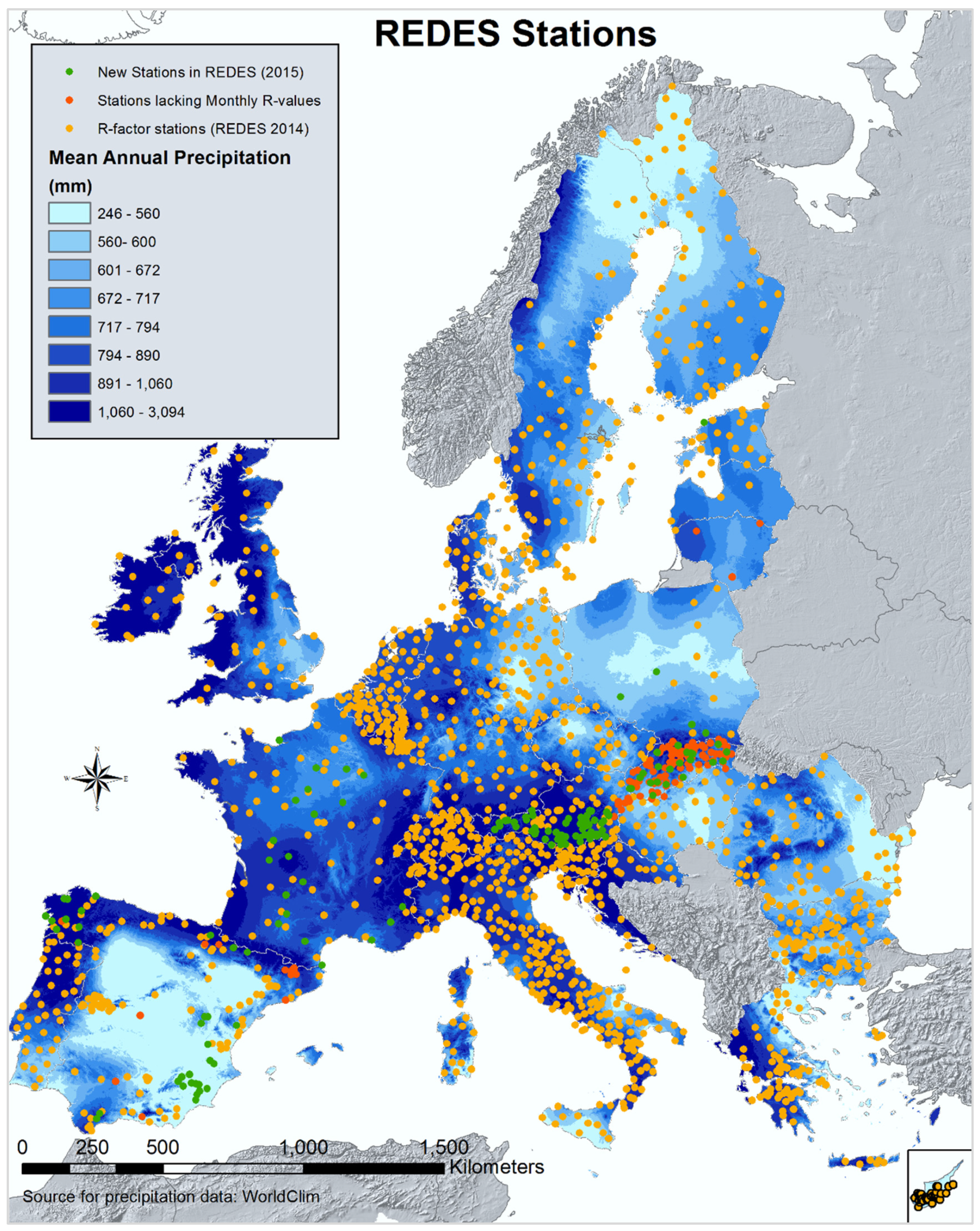
2. Materials: Rainfall Erosivity Database at European Scale (REDES) and 2015 Updates

The first version of the Rainfall Erosivity Database at the European Scale (REDES) included 1541 rainfall stations within the European Union (EU) and Switzerland [7]. The rainfall erosivity has been calculated in REDES by using high temporal resolution data (5-min, 10-min, 15-min, 30-min and 60-min) for periods ranging from 7 to 56 years (average length 17.1 years) and applying the equations proposed by Brown and Foster [8]. The rainfall erosivity map of Europe and other derived datasets (erosivity density, standard error) are available for download from the European Soil Data Centre (ESDAC). Due to space constraints, here we limit the description of the REDES database development and characteristics; for further details on REDES, the input rainfall data, the data availability and the updates, please see Panagos et al. [7] and Panagos et al. [9].

In 2015, REDES was updated by adding 134 new rainfall stations (8.5% increase). In Austria, 53 stations were added mainly covering the southern regions of the country (Tyrol and Carinthia), where the R-factor has been measured to be larger than 4000 MJ mm·ha⁻¹·h⁻¹·year⁻¹ (Nassfeld station) [9]. In Slovakia, 22 stations were added to REDES, as the existing 81 stations had only annual R-factor values from the literature. Finally, 21 stations (well distributed in the country) were added in France, 4 stations in Poland and 33 stations in 4 Spanish catchments (Galicia, Júcar, Ebro and Hidrosur) (Figure 1).

The main objective of the REDES update (during 2015) was to cover areas with data gaps (Poland, Spain, South Austria, and France) and to insert new data where seasonal R-factor values were not available (Slovakia). The updated REDES included 1675 rainfall stations with high-resolution rainfall data. Monthly R-factor values have been calculated for the 1568 stations out of 1675 as the rest of the stations (107) have only annual R-factor values retrieved from the literature.

3. Methods

The data collection of the high-temporal-resolution rainfall records has been explained in Panagos et al. [7]. After the recent REDES update with the new 134 records, the methods include three further steps: (a) calculation of monthly erosivity values per station; (b) normalization of R-factor values calculated using rainfall data with different time steps (5 to 60 min); and (c) spatial analysis of intra-annual (monthly) rainfall erosivity and erosivity density.

3.1. Monthly R-factor Calculation

Despite the high importance of seasonal rainfall erosivity variation, few studies have analyzed its inter-annual and spatial variability [10,11,12,13]. In the calculation of the original REDES dataset and in the present paper, we have applied the rainfall energy equation proposed by Brown and Foster [8] for the R-factor calculation and followed the criteria for the identification of erosive events [4]. This methodology is briefly described as follows.

The R-factor is the product of the kinetic energy of a rainfall event (E) and its maximum 30-min intensity (I₃₀):

$$R=\frac{1}{n}{\displaystyle \sum }_{j=1}^n{\displaystyle \sum }_{k=1}^{m_j}{\left(E{I}_{30}\right)}_k$$

(1)

where R is the average monthly rainfall erosivity (MJ·mm·ha⁻¹·h⁻¹·month⁻¹), n is the number of years recorded, m_j is the number of erosive events during a given month j, and EI₃₀ is the rainfall erosivity index of a single event k.

The erosivity of a single event EI₃₀ (MJ mm ha⁻¹ h⁻¹) is defined as:

$$E{I}_{30}=\left({\displaystyle \sum }_{r=1}^m{e}_r v_e\right)I_{30}$$

(2)

where e_r is the rainfall kinetic energy (MJ·ha⁻¹·mm⁻¹) and v_r is the rainfall volume (mm) during the r-th period of a storm that is divided into m-parts.

The rainfall kinetic energy (e_r) per rainfall depth (mm) and per unit area (ha) for each time interval is calculated as follows [8]:

$$e_r=0.29\left[1-0.72\text{exp}\left(-0.05i_r\right)\right]$$

(3)

where i_r is the rainfall intensity during the time interval (mm h⁻¹).

The sums of EI₃₀ and the average R-factor have been calculated on a monthly basis. To compute the R-factor, the erosive rainfall events (m_j) for each station have been selected based on thresholds set by Renard et al. [4] followed by Panagos et al. [7]. The Rainfall Intensity Summarisation Tool (RIST) software [14] has been used to calculate the R-factor. Moreover, this tool also derives the monthly R-factor values, allowing us to build the monthly “dimension” in REDES. Our database with monthly average erosivity values is made up of 12 monthly values per 1568 stations (i.e., 18,816 records).

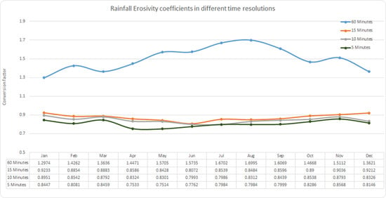
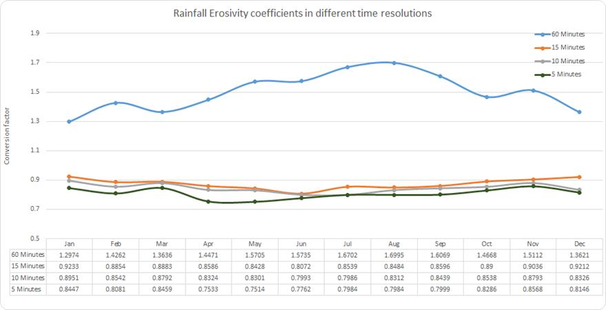
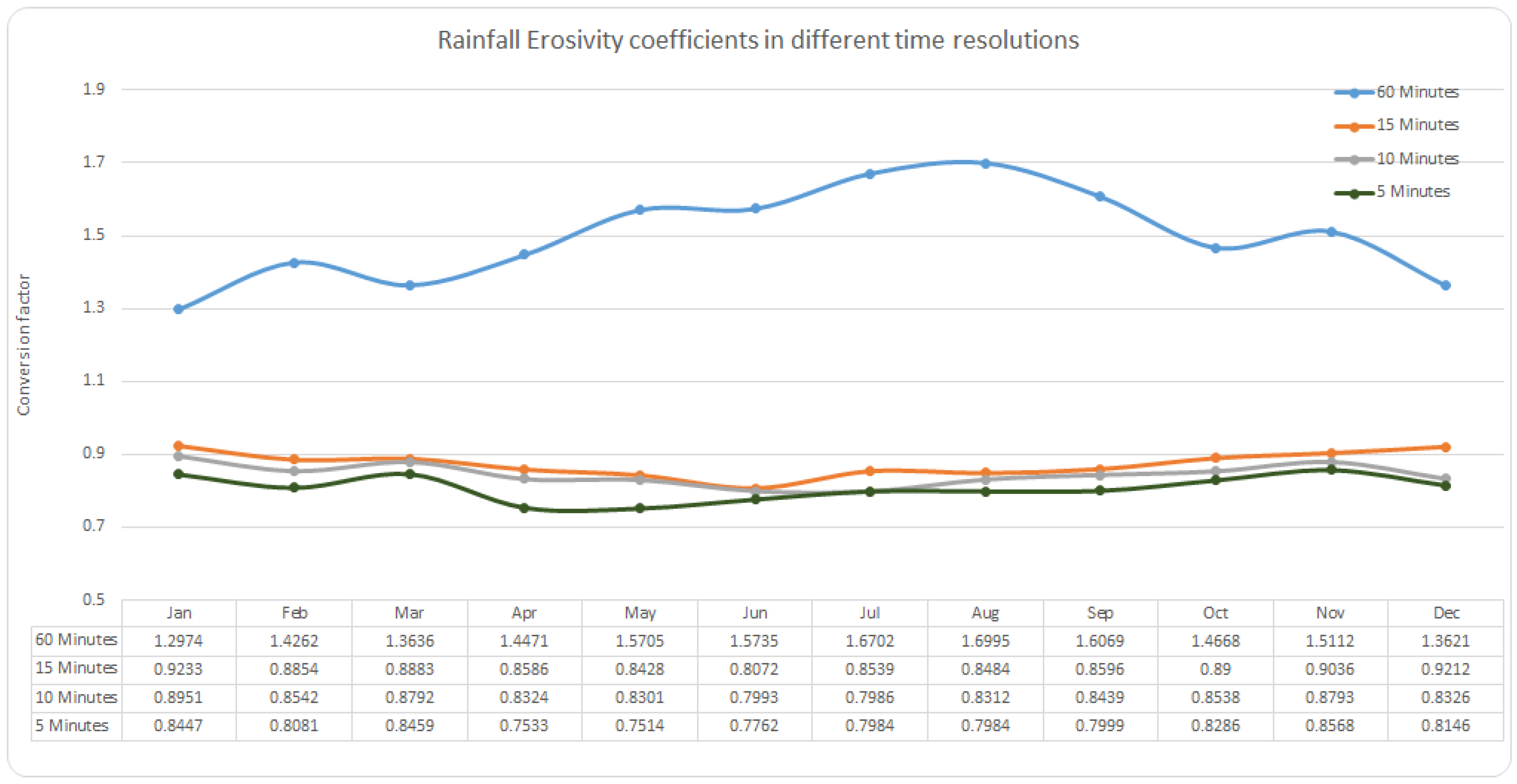
3.2. Calibration of Monthly R-factors Calculated from Different Temporal Resolution Rainfall Data

The objective of this calibration is to account for the impact of differences in the time resolution of rainfall records on rainfall erosivity, and furthermore to develop calibration functions making the REDES homogeneous at a common time resolution of 30-min. The issue of different time resolutions for R-factor estimation has been faced in the past as well. Weiss [15] estimated the conversion factor between EI₃₀ and EI₁₅ at 1.0667. In the United States, Renard et al. [4] developed a range of coefficients varying from 1.08 to 3.16 in order to “transfer” R-factor values calculated on an hourly basis to 30 min R-factor values based on measurements from 713 stations. Yin et al. [16] calculated the conversion factors between different resolutions based on measurements of 5 stations in China. Agnese et al. [17] also estimated the R-factor at 3 different resolutions (5-min, 15-min, and 60-min) for 7 stations in Sicily (Italy). In the European Union, Panagos et al. [7] developed calibration functions based on R-factor estimations at 5 different resolutions (60-min, 30-min, 15-min, 10-min, and 5-min). According to the REDES statistics, 23.4% of the European stations have rainfall data at very high resolution (<15 min). Taking into account this fact, the calibration functions are necessary to provide consistent estimations of the R-factor for a wide area such as Europe.

The REDES database includes stations that have different recording intervals: 60 min, 30 min, 15 min, 10 min and 5 min. A calibration procedure has been followed for transforming the R-factor values to a common time resolution of 30 min. In this way, REDES becomes homogenous in terms of time resolution, and allows assessments of annual and monthly erosivity. Using a geographically representative pool of rainfall stations with different time resolutions, four calibration functions have been produced in order to ‘transform’ the R-factor values to 30-min resolution [7]. The calibration process included the following steps:

-

The R-factor was calculated at the highest available resolution (i.e., <30 min) for a number of stations (86 stations well distributed across Europe).

-

Data have been aggregated to coarser resolution(s) and the R-factor was calculated at the coarser resolution for the same stations.

-

A calibration function, derived from regression analysis, has been developed based on the R-factor results at the highest possible resolution and the coarser resolution(s).

The four calibration functions were derived from the annual R-factor values and are applicable for the normalization of annual erosivity. Since the R-factor has different monthly patterns—due to the different monthly precipitation regimes—the annual regression functions would be inappropriate for the calibration of monthly R-factor values. Thus, we decided to develop calibration functions per month, following the same procedure as in the calibration of annual R-factor values. Those calibration functions have been developed for each month and for all applied resolutions (5-min, 10-min, 15-min and 60-min). The pool of rainfall stations involved in this calibration exercise was selected because of their data availability at multiple temporal resolutions. Moreover, the pool well represents the study area (stations from 14 countries: Belgium, Czech Republic, Switzerland, Cyprus, Germany, Estonia, Spain, France, Croatia, Hungary, Italy, Luxembourg, Romania, Slovenia) and their data recordings cover the last 10–25 years.

In an ideal situation where rainfall data at very high resolution (<15 min) could be available for all European countries, the calibration functions could be estimated even per climatic zone in Europe. For example, you cannot develop calibration functions per climatic region for the 15-min resolution when rainfall data at this scale are available only for Spain and Belgium. The same applies for the calibration functions for the 10-min resolution as the rainfall data at this scale are available for 4 countries (Croatia, Hungary, Romania and Switzerland) (Table 1 in [7]). Due to exceptional requests to the Environmental and Climatic services in Czech Republic, Cyprus, Germany, Estonia and Luxembourg, the pool of stations with 10-min rainfall data included 9 countries well-distributed in Europe (Table 2 in [7]) and allowed us to develop calibration functions at the European scale. Considering the potential of the REDES database, as further improvements, we plan exploring the possibility to obtain conversion factors that vary from region to region, and even enlarge the sample data for regression analyses.

The REDES database includes stations whose data spans from 7 to 56 years, thus covering a temporal period of many decades, from the 1960’s to the last decade. This period is well known to have been undergoing climate change, in particular the last three decades, which experienced a global warming trend and a more pronounced rate of rainfall extreme events that involved Europe as well [18,19]. Though the preliminary tests we performed, it was proved that the monthly calibration functions show slight differences if computed using stations with different periods of data. Thus, we decided to use input data from the latest 25 years, in order to avoid possible biases introduced by different temporal rainfall regimes. Moreover, choosing the latest years, it follows that the calibration functions are effectively representing the physical characteristics of the last decade; consequently, the applications of such factors can be extended to newly collected data. We also highlight that, based on our tests, monthly conversion factors are more subject to spatial rainfall patterns than temporal issues, provided that the input data used to calculate them range over a sufficiently long period (i.e., 20 years) [9].

4. Results and Discussion

4.1. Regression Curve for Annual R-factor Value

In addition to the 4 calibration functions proposed by Panagos et al. [7], stations with data at very high resolution (1-min) from the Czech Republic and Slovakia have been used. The R-factor calculated with 30-min data is 0.7496 times lower than the R-factor calculated at 1-min data and 1.5597 times higher than the R-factor calculated at 60-min data. The term ‘calibration factor’ is used below to represent this conversion between the R-factor at different resolutions and the R-factor at 30-min. Based on the six calibration factors at the corresponding time resolutions (1, 5, 10, 15, 30 and 60-min), a regression function has been developed (Figure 2). The limited number of calibration factors is a source of uncertainty and the regression function should be handled with care and used only for the entire study area. The regression function allows estimating calibration factors at every temporal resolution between 1 and 60 min, though it is uncommon to use rainfall data at time resolutions different from those shown in Figure 2.

The results of the annual calibration showed that the calibration factors in Europe are closer to the smallest values obtained by Renard et al. [4]. The estimated calibration factors match well with the findings in Sicily [17], Calabria [20], United States [6,21], and they are 10%–20% larger than the ones estimated in China [16]. However, not only the precipitation regimes of China (e.g., [22,23]) are remarkably different from the corresponding European ones [24], but also the general physical, climatic, and hydrological features are dissimilar compared to European ones ([25,26]); thus, similar calibration factors are not to be expected.

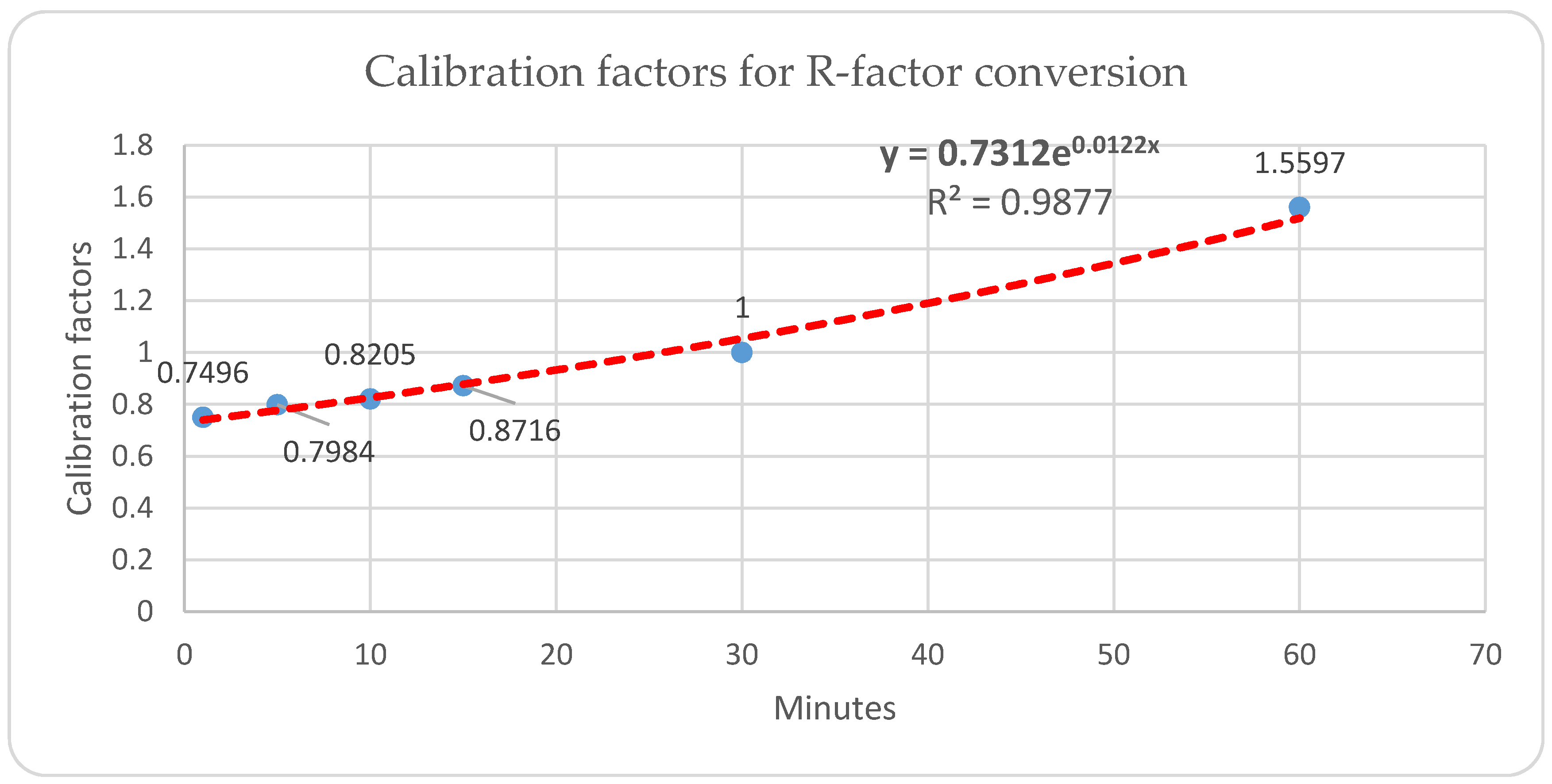
4.2. Monthly Calibration Factors for Different Temporal Resolution

The annual calibration factor for the R-factor estimation using the 60-min data has been estimated to be 1.5597, ranging from 1.2974 (January) to 1.6995 (August). The smallest calibration factors are estimated in winter, while the largest ones are found in summer (Figure 3). Compared with using one single calibration factor for the whole year, the option to apply monthly calibration factors is recommended, as there is 25% variability in the monthly conversion factors.

The annual calibration factor for estimating an annual R-factor by using 10-min data has been estimated at 0.8205, ranging from 0.7986 (July) to 0.8951 (January). The smoothest calibration factors (closer to 1) are found in winter. The monthly conversion factors allow us to reallocate the R-factor at the desired resolution even if the data are available at coarser resolution. For example, the August R-factors at 60-min can be converted to 5-min by multiplying them by a factor 2.13, while the January ones are multiplied by a factor 1.54 (Figure 3). In addition, the calibration factors between very high-resolution (e.g., between 15-min and 5-min) vary between 1.05–1.12 for the different months.

The good performance in terms of coefficient of determination (R²) in both the annual calibration functions and in the monthly ones permitted us to develop general pan-European calibration functions (Figure 3) that can be used in regional assessments in the case that better data than REDES are not available.

As the number of stations with available data at different time resolutions was 86 across Europe, it was impossible to develop regression functions per climatic region and per time resolution. Even if each climatic zone may have slightly different calibration functions, the objective of this study was to focus at the European scale (Figure 3).

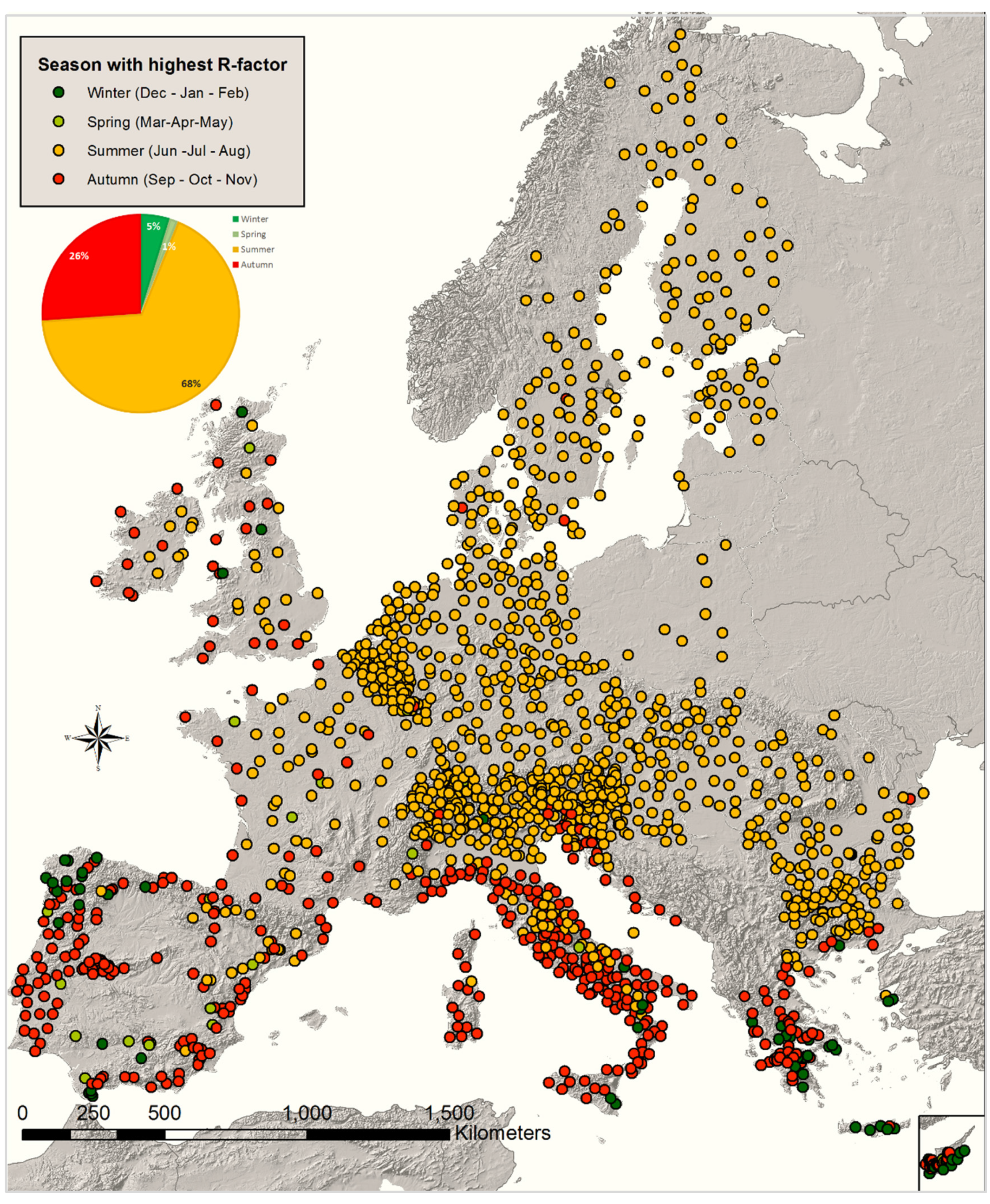
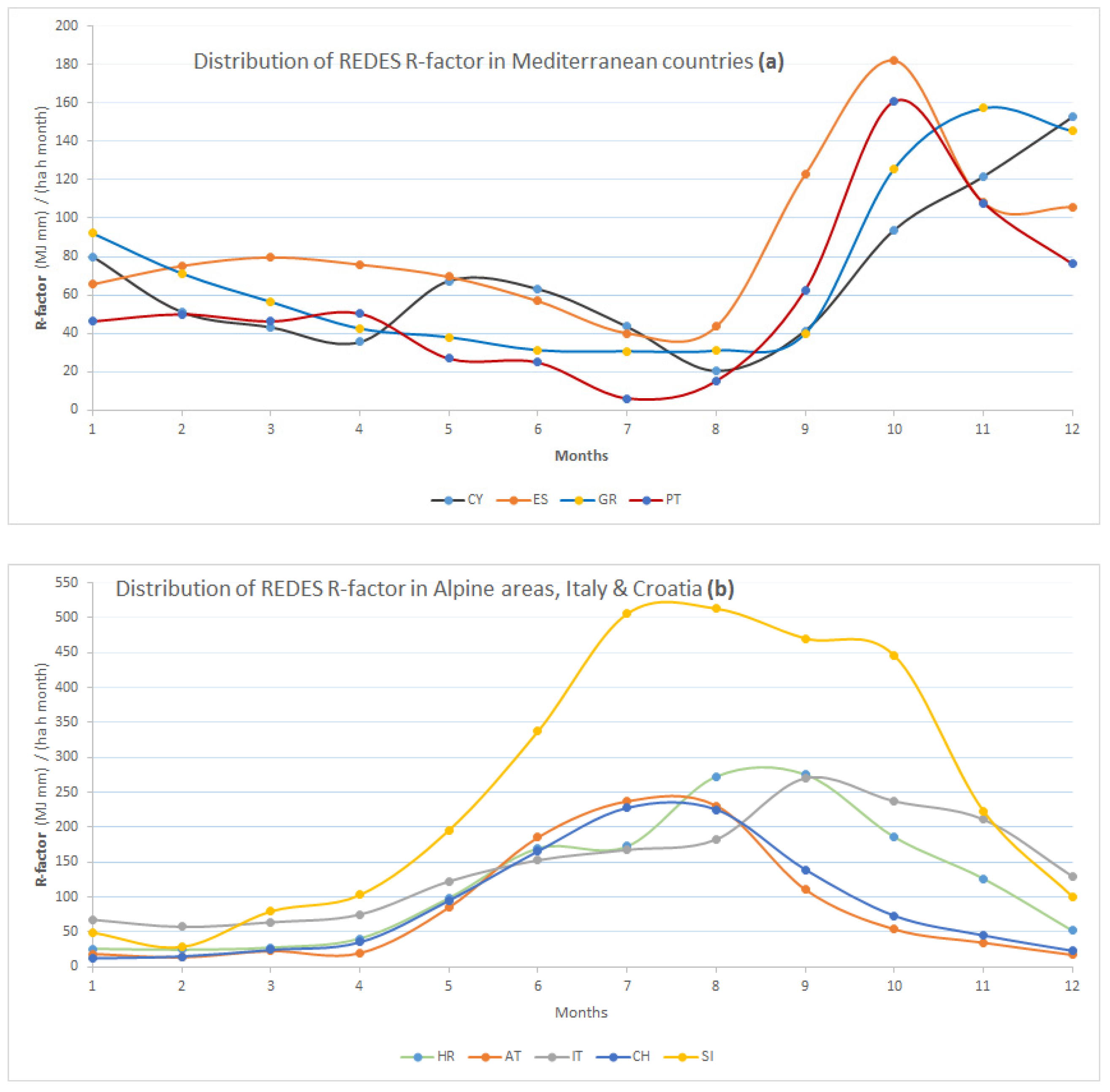
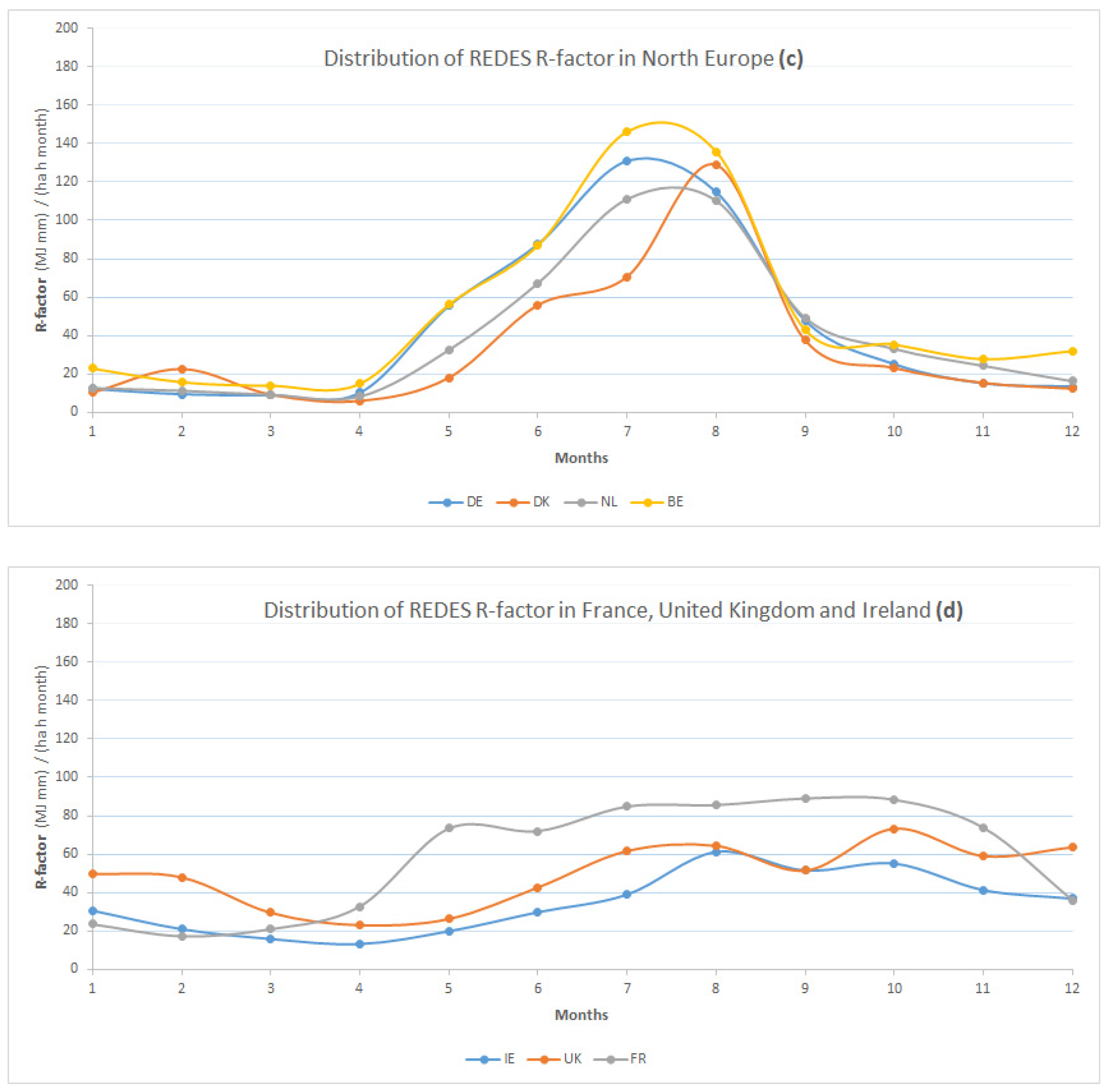
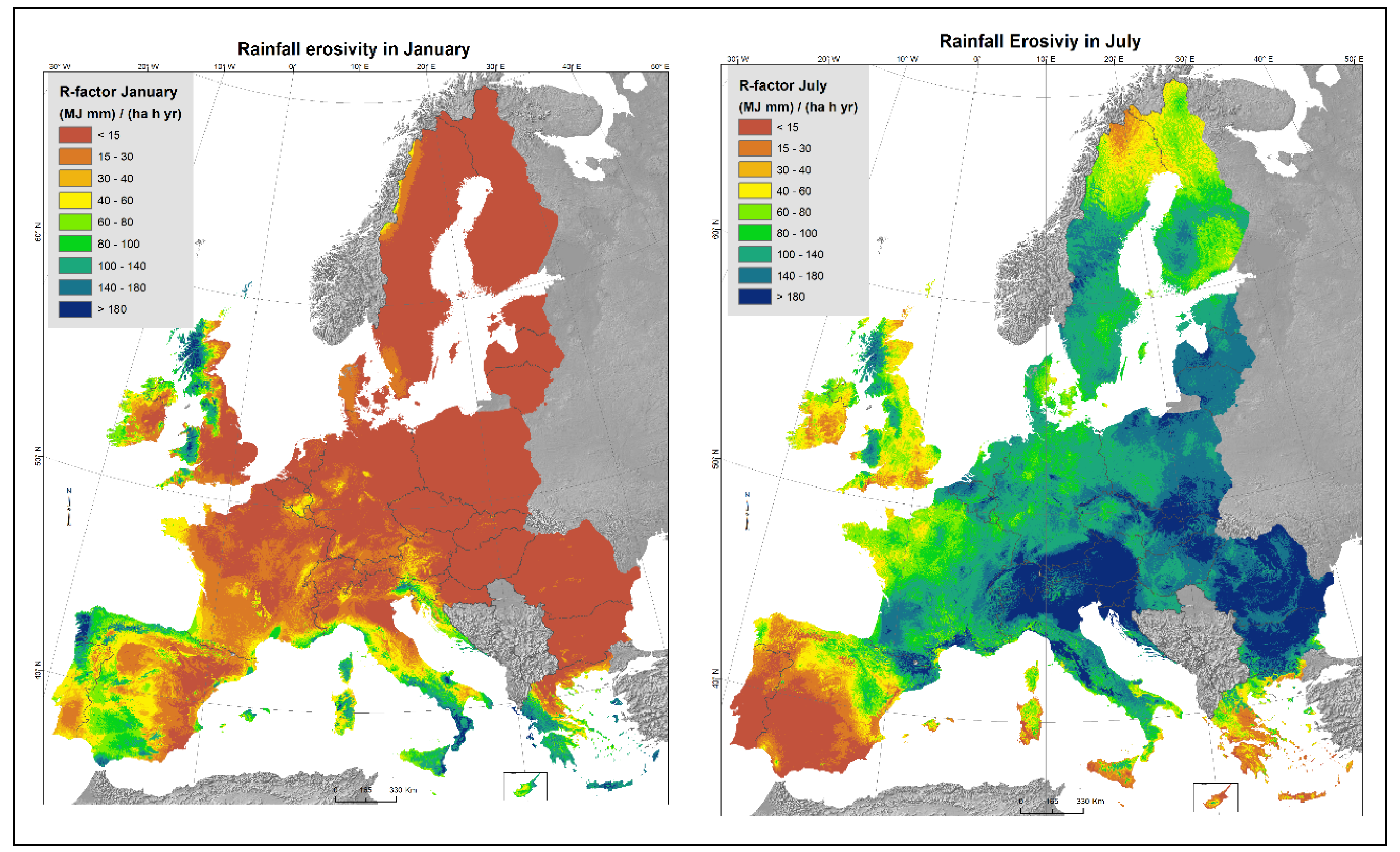
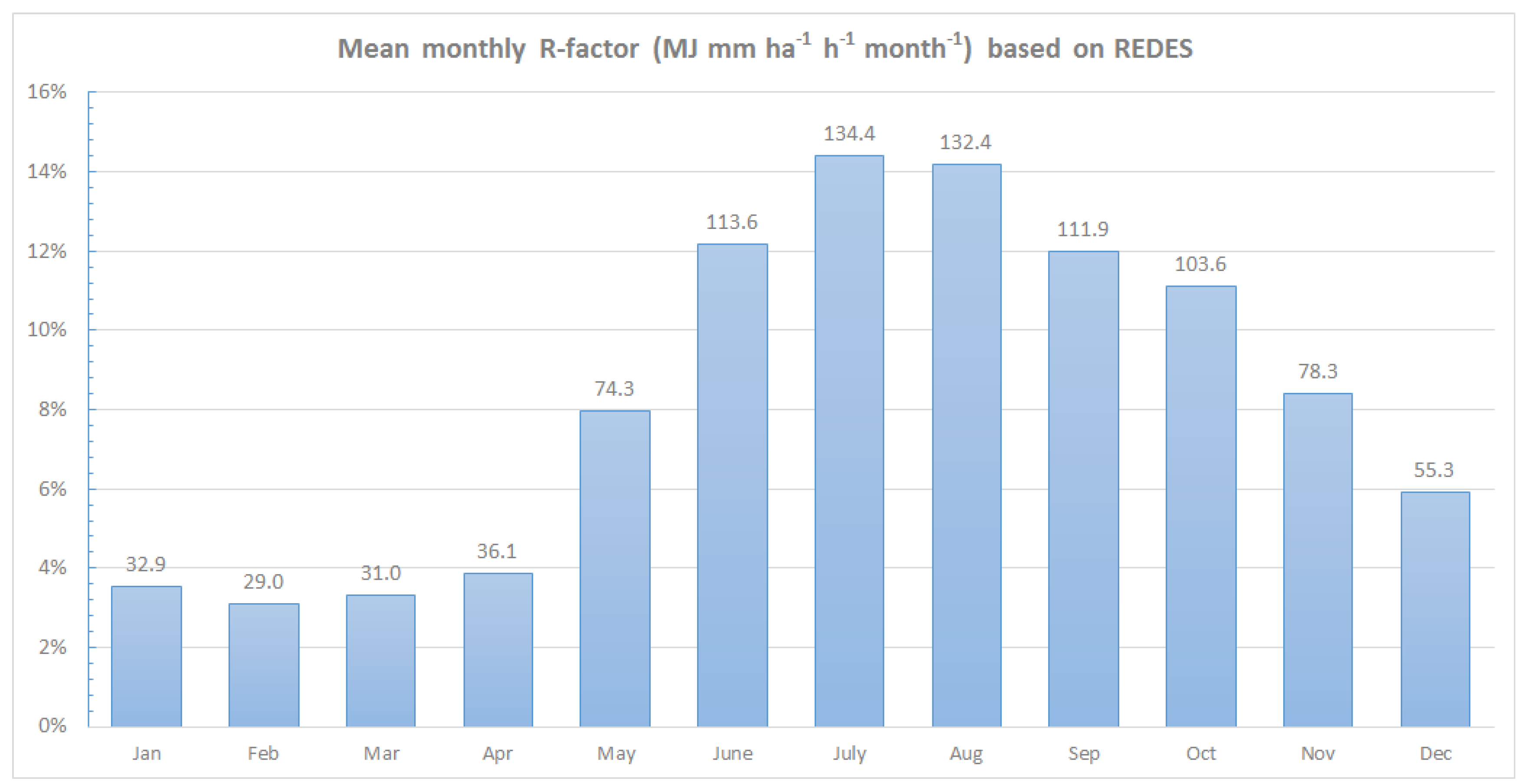
4.3. Seasonal and Monthly Rainfall Erosivity

The annual R-factor map of Europe [7] gives a spatial overview of the potential of rain to cause erosion and allows identification of hot-spots where intervention may be needed. However, the control measures (agricultural, crop management and support practices) can be more efficient if the temporal distribution of rainfall erosivity is known. The temporal analysis of the two dynamic erosion factors (rainfall erosivity and cover-management) is important to take control measures against erosion [27]. Most of the RUSLE applications worldwide did not take into account the temporal variability of these two factors despite those intra-annual dynamics being documented in the RUSLE manual [4]. The monthly R-factor in combination with a future pan-European study on modeling seasonal cover-management represents a relevant step ahead in the framework of soil loss monitoring at the European scale [28]. This can be achieved by modifying the classical RUSLE approach to estimate average annual soil loss and propose the seasonal erosivity [29] in combination with intra-annual land cover variability and closer monitoring of management practices. Increasing availability of remote sensing data on land cover and vegetation (e.g., COPERNICUS programme; [30]) can contribute to a seasonal estimation of a cover-management factor.

The mean R-factor of the updated REDES (1675 stations) is 906 MJ·mm ha⁻¹ h⁻¹ year⁻¹; close to the one estimated in 2014. The monthly R-factor was calculated for 1,568 stations only due to the lack of monthly R-factor values at 107 stations whose annual R-factor values have been retrieved from the literature. The stations excluded are mainly located in Slovakia (81 stations), Spain and Lithuania and have small rainfall erosivity values. Those excluded small values have a small effect in aggregating slightly larger mean monthly R-factors values.

July and August are the months in which the highest number of intense erosive events occur in Europe (Figure 4). More than 40% of total rainfall erosivity in the European Union and Switzerland takes place in the summer period and more than 53% is noticed during the period June–September. According to the monthly distribution of rainfall erosivity in Europe, the mean R-factor does not show significant variations during the first four months (January to April) of the year, followed by a remarkable linear increase until July/August (Figure 4). Finally, a smoother decrease, compared to the summer increase, is noticed during autumn and continues until February.

Within Europe, geographic differences exist in the seasonal patterns of rainfall erosivity. The stations with the absolute largest R-factor value in a single month (for instance July, August, September or October) are located mostly in Italy and Slovenia. For each REDES station, the season (spring, summer, autumn, winter) with the largest R-factor has been selected (Figure 5). For 94% of the REDES stations, the most erosive period is either summer (68%) or autumn (26%). For only 22 REDES stations, mainly located in South Spain and France, the most erosive period is spring (Figure 5).

During summer, the R-factor exhibits its largest seasonal values for stations located in Northern European countries, i.e., the Baltic States, Scandinavia, Central and Eastern Europe, the Alpine region and the Apennines, as it can be seen from the distribution of the seasons with the largest R-factor values (Figure 5). This zone covers the largest part of Europe. A second zone, where autumn is the most erosive period, includes parts of the Mediterranean basin (Western Greece, coastal Italy, south France, Portugal and major part of Spain, Croatia and coastal Slovenia). As the Mediterrean basin has a complex morphology (e.g., sharp orographic features), there areas where stations with the highest R-factor values in all seasons are close to each other. A third zone, where winter is the most erosive period is limited to Cyprus, Crete, part of Greece and Galicia. Finally, a mixed situation where summer and autumn are dominant erosive periods is noticed in United Kingdom, Ireland and part of North France. On average, more than 55% of the total annual R-factor [E1] takes place in only one season.

The R-factor shows the largest monthly values in autumn across most of the Mediterranean region, where the precipitation amount is generally larger in October–November [31,32] and summers are frequently hot and dry [33]. Southern Greece and Cyprus can be considered to be an exception in R-factor patterns of the Mediterranean region, as the rainfall erosivity peaks in winter and it is small in spring even if those regions show a similar rainfall amount compared to autumn [34].

The Atlantic regions do not show distinctive patterns, probably because the monthly precipitation variability is smaller than in the continental regions [35], especially in the British Islands [36,37]. The R-factor is largest in summer in Central Europe, Northern Europe, Eastern Europe and the Alps. This pattern might have different explanations, as Central Europe is generally affected by large-scale extreme precipitation events in summer [38], while the Alps are usually affected by local summer thunderstorms and rain showers, due to the remarkable temperature gradients between hot and moist lowlands and cool and windy mountains [11,39,40]. Similar patterns can be found in the Carpathians and Eastern Europe [41,42,43]. Finally, Scandinavia shows higher variability in summer, but one should not forget that in winter, the precipitation events at high-latitudes are often in the form of snowfall and so we expect much fewer erosive events in winter compared to summer [44]. The stations with an almost zero R-factor during winter months are located in Central and Eastern European countries (Czech Republic, Slovakia, Bulgaria, and Romania) and in the Northern ones (Sweden and Finland).

Regarding the most erosive months for single stations, we found that in almost 30% of REDES, the most erosive month is July, followed by August (23.7%) and June (12.7%). On the contrary, the months with the least number of stations having the largest R-factor values are April and March. On average, the most erosive month of the year accounts for 28% of the total annual erosivity. In the Baltic and high-latitude regions, the most erosive month (either July or August) accounts for more than 38% of the annual R-factor. Lastly, the situation is much smoother in Ireland where the most erosive month is not a peak as it contributes only 16% to the total annual erosivity.

Besides the most erosive season or the most erosive month (in terms of R-factor), it is worth identifying the different intra-annual patters of the R-factor in the European continent. Most of the countries have been grouped based on their geographical position and their monthly patterns of rainfall erosivity (Figure 6). The distribution of the monthly erosivity in the Mediterranean countries (Spain, Portugal, Greece and Cyprus) (Figure 6a) follows a bathtub shaped curve [45], as three periods can be identified. Rainfall erosivity is more or less stable in the period from February to June and then shows a decrease in July and August (second period). Finally, December is the most erosive in Greece and Cyprus, while October has the largest values in the Iberian Peninsula (Figure 6a).

The temporal distribution of rainfall erosivity is very similar in Switzerland and Austria (Figure 6b), having the largest values in July and August. Instead, Northern Italy and Croatia show their peak values in September. These countries have the largest mean monthly values in REDES.

In Germany, The Netherlands, Belgium and Denmark, the rainfall erosivity is very limited during winter and early spring, then increases in May-June-July (and August in Denmark), followed by a sharp decrease in autumn (Figure 6c). The monthly R-factor distribution follows a Gaussian shape [46] in Germany, The Netherlands, Belgium and Denmark. Contrary to the three above-mentioned regional patterns (Mediterranean, Alpine, North Europe), Ireland, United Kingdom and France show the smoothest distribution during the whole year (Figure 6d).

The remaining countries (Scandinavia, Baltic States, and Central Europe) follow the distribution identified in North Europe (The Netherlands, Germany, Denmark), as shown in Figure 6c. Using the Cubist spatial interpolation model [47], we have developed the first predictions of monthly erosivity maps. The R-factor maps of January and July (Figure 7) usually represent opposite winter and summer peak values. This is a first important application of the monthly REDES regarding the monthly conversion factors and the derived monthly rainfall erosivity maps.

The magnitude of predicted climate change is likely to have a different influence on soil erosion depending on regional conditions [48,49]. As the predictions in climate change scenarios are expected to increase the number of storms during the summer months [18,50], the countries with large erosivity during summer are projected to be more affected. However, the projected rainfall erosivity changes in Europe based on Intergovernmental Panel on Climate Change (IPCC) climatic change scenarios and REDES are planned in the near future.

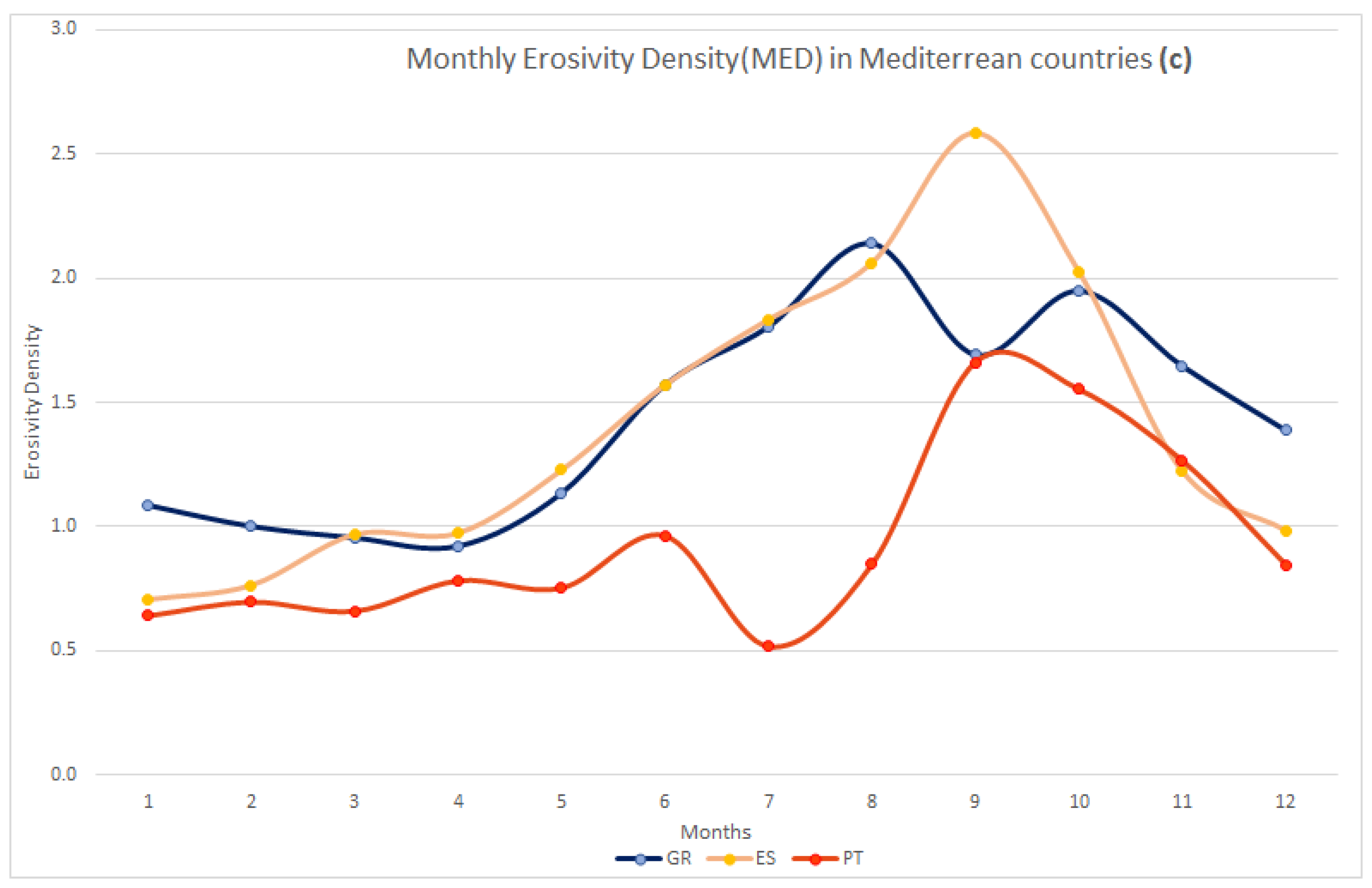
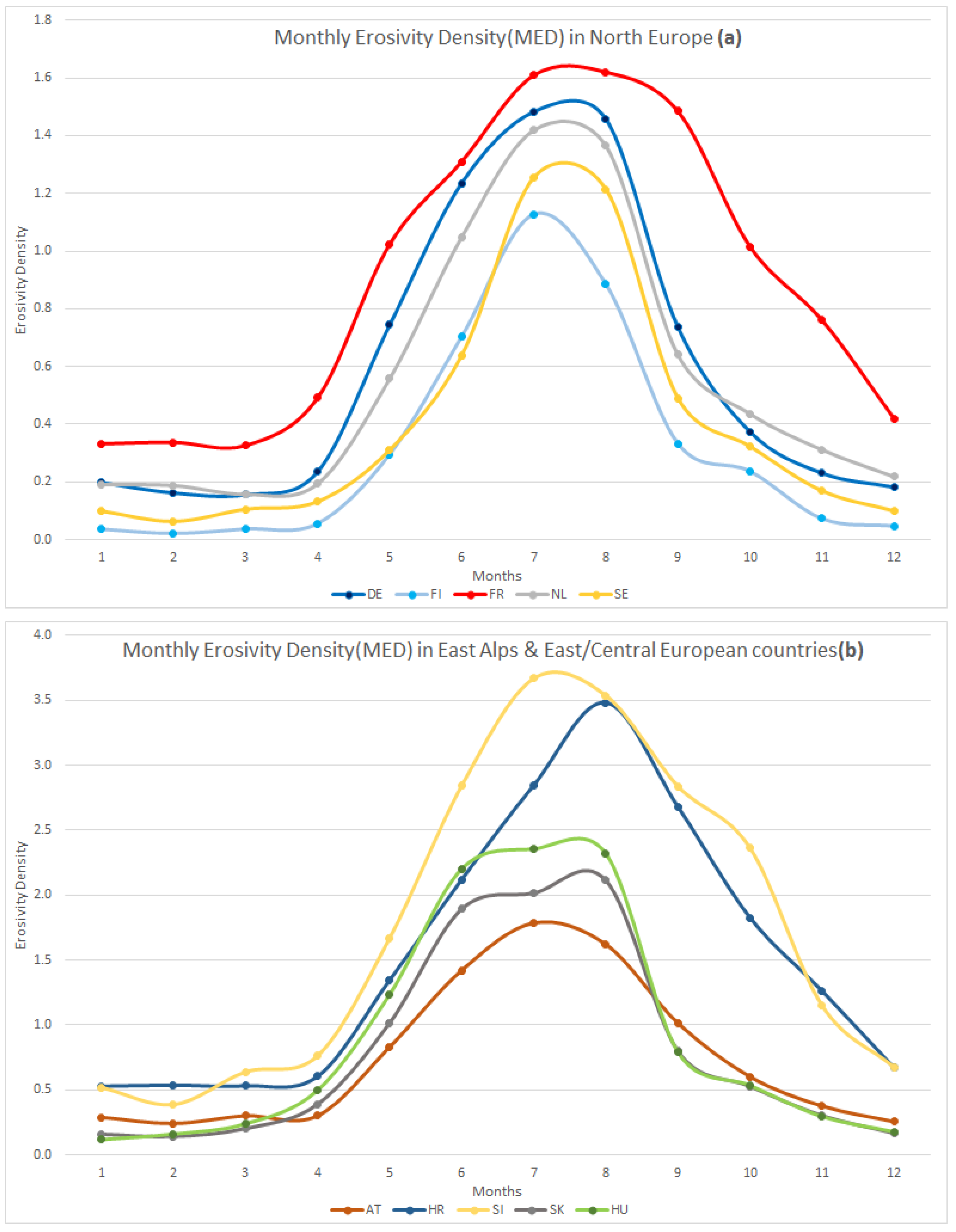
4.4. Monthly Rainfall Erosivity Density

Similar to annual erosivity density [7,51,52,], the Monthly Erosivity Density (MED) expresses the rainfall erosivity per rainfall unit (mm) for each month. The erosivity density is highly reliant on rainfall intensity and, on event basis, influences event sediment concentration (soil loss per unit quantity of water). Dabney et al. [53] used the monthly erosivity density to demonstrate the impact of climate change in increasing runoff and soil loss. For each station in REDES, the Monthly Erosivity Density (MEDi) for the i-th month is defined as the ratio of mean rainfall erosivity (R) for the i-th month divided by its mean precipitation (P):

$$ME{D}_i=R_i/P_i$$

(4)

Large MED values suggest that rainfall occurs in the form of high intensity events (rainstorms) during the respective month. The distribution of MEDs in Europe is left skewed. Half of the monthly REDES records have an erosivity density smaller than 0.45, while the 75th percentile is close to 1.

Some countries have similar characteristics regarding their MED and the corresponding monthly variability. For example, for all months, the mean MED in Sweden, Finland, Denmark, Germany, Netherlands, France, Ireland and United Kingdom is less than 1.62 (Figure 8). In these countries, MED is always smaller than 0.40 in winter—early spring (December, January, February, March, April). For these eight countries, the largest MED can be found either in July or August varying from 0.57 (Ireland) to 1.62 (France).

The Northern European countries show similar monthly variability regarding erosivity density (Figure 8a). The Gaussian distribution of mean monthly erosivity density is represented with the “bell-shaped curve”, increasing during May to June, reaching its largest in July and then having a sharp decrease during early autumn. In France, the larger values of MED are due to larger R-factor values in the Alpine areas.

The mean MED reaches the largest values (close to 3.67 during summer) in the Eastern Alps (Slovenia, North-East Italy) and Croatia; in Central European countries (Austria, Slovakia, and Hungary), the mean MED is larger than 1.65 during summer (Figure 8b). In all of these countries, the winter and early spring are characterized by a relatively small MED (<0.75).

In Ireland and the United Kingdom, MEDs are very smooth compared with the rest of European countries and have values ranging between 0.19 (April) to 0.78 (July). The Mediterranean countries are quite different from the rest of the European countries, as their largest MED is found in September or August (Figure 8c). Moreover, the winter months in Spain and Greece have MEDs close to 1, which is not noted in Northern Europe.

5. Conclusions

In this study, calibration factors for transferring the R-factor values between different time resolutions on a monthly scale have been produced; these can be applied in case of monthly or annual estimation of R-factors in any part of Europe. As expected, the calculated rainfall erosivity values decrease as the rainfall measurement interval increases. According to our analyses, the relationship between time resolution and conversion factors is exponential, different from past assessments that proposed linear functions [4,16]. The coefficients of different resolutions for monthly rainfall erosivity allow normalizing the monthly R-factor values to a common 30-min resolution for all the REDES stations. The development of the monthly dimension in the REDES database allows the assessment and modeling of the R-factor at the monthly and seasonal levels.

Compared to the study of Diodato and Bellocchi [54], who investigated the decadal rainfall-runoff erosivity in Central Europe and the Mediterranean region, this study is based on a larger input dataset, introduces a different methodology, analyzes the rainfall erosivity spatial patterns on a monthly basis and covers a much wider area (European Union plus Switzerland). One of the most relevant findings is the assessment of the regions that can be considered under threat from rainfall erosivity: the Alpine region is characterized by high erosivity during summer and early autumn (July to September), while the Mediterranean region has its largest peaks in late autumn and early winter. Consideration of monthly rainfall erosivity patterns is crucial for landscape and catchments management for an optimization of agricultural land use (vegetation cover, support practices) and natural hazard prediction (soil erosion, landslides and floods).

For instance, it is important to maintain vegetation coverage in Central and Northern European countries during summer months while October to December is the most critical season for Mediterranean countries. Identifying the most erosive season (month) per country (region) can contribute to mitigate soil erosion by protecting soil with vegetation coverage and applying appropriate management practices. As topography and soil properties are soil erosion drivers that are more constant over time, the vegetation coverage and crop management are the factors that can be primarily influenced by human intervention.

Finally, the new proposed monthly erosivity density index identifies the most risky seasons in terms of floods and erosive events, as large monthly erosivity density values correspond to seasons and areas with high intensity of rainfall creating extreme erosive events. Based on this index, the erosive events in summer months in the Eastern Alps and Central Europe and in autumn in the Mediterranean area may lead to R-factor values that range from two to four times the corresponding rainfall amounts.

References

1. Lal, R. Soil degradation by erosion. Land Degrad. Dev. 2001, 12, 519–539. [Google Scholar] [CrossRef]
2. Panagos, P.; Meusburger, K.; Van Liedekerke, M.; Alewell, C.; Hiederer, R.; Montanarella, L. Assessing soil erosion in Europe based on data collected through a European Network. Soil Sci. Plant Nutr. 2014, 60, 15–29. [Google Scholar] [CrossRef]
3. Wang, G.; Gertner, G.; Singh, V.; Shinkareva, S.; Parysow, P.; Anderson, A. Spatial and temporal prediction and uncertainty of soil loss using the revised universal soil loss equation: A case study of the rainfall-runoff erosivity R factor. Ecol. Model. 2002, 153, 143–155. [Google Scholar] [CrossRef]
4. Renard, K.G.; Foster, G.A.; Weesies, G.A.; McCool, D.K.; Yoder, D.C. Predicting Soil Erosion by Water: A Guide to Conservation Planning with the Revised Universal Soil Loss Equation (RUSLE); Agricultural Handbook 703; US Department of Agriculture: Washington, DC, USA, 1997; pp. 1–404.
5. Wischmeier, W.; Smith, D. Predicting Rainfall Erosion Losses: A Guide to Conservation Planning; Agricultural Handbook No. 537; U.S. Department of Agriculture: Washington, DC, USA, 1978.
6. Istok, J.D.; McCool, D.K.; King, L.G.; Boersma, L. Effect of rainfall measurement interval on EI calculation. Trans. Am. Soc. Agric. Eng. 1986, 29, 730–734. [Google Scholar] [CrossRef]
7. Panagos, P.; Ballabio, C.; Borrelli, P.; Meusburger, K.; Klik, A.; Rousseva, S.; Tadic, M.P.; Michaelides, S.; Hrabalíková, M.; Olsen, P.; et al. Rainfall erosivity in Europe. Sci. Total Environ. 2015, 511, 801–814. [Google Scholar] [CrossRef] [PubMed]
8. Brown, L.C.; Foster, G.R. Storm erosivity using idealized intensity distributions. Trans. ASAE 1987, 30, 379–386. [Google Scholar] [CrossRef]
9. Panagos, P.; Meusburger, K.; Ballabio, C.; Borrelli, P.; Begueria, S.; Klik, A.; Rymszewicz, A.; Michaelides, S.; Olsen, P.; Tadic, M.P.; et al. Reply to the comment on “Rainfall erosivity in Europe” by Auerswald et al. Sci.Total Environ. 2015, 532, 853–857. [Google Scholar] [CrossRef] [PubMed]
10. Diodato, N. Predicting RUSLE (Revised Universal Soil Loss Equation) monthly erosivity index from readily available rainfall data in Mediterranean area. Environmentalist 2006, 26, 63–70. [Google Scholar] [CrossRef]
11. Meusburger, K.; Steel, A.; Panagos, P.; Montanarella, L.; Alewell, C. Spatial and temporal variability of rainfall erosivity factor for Switzerland. Hydrol. Earth Syst. Sci. 2012, 16, 167–177. [Google Scholar] [CrossRef] [Green Version]
12. Sadeghi, S.H.R.; Hazbavi, Z. Trend analysis of the rainfall erosivity index at different time scales in Iran. Nat. Hazard. 2015, 77, 383–404. [Google Scholar] [CrossRef]
13. Panagos, P.; Ballabio, C.; Borrelli, P.; Meusburger, K. Spatio-temporal analysis of rainfall erosivity and erosivity density in Greece. Catena 2016, 137, 161–172. [Google Scholar] [CrossRef]
14. Klik, A.; Konecny, F. Rainfall erosivity in northeastern Austria. Trans. ASABE 2013, 56, 719–725. [Google Scholar] [CrossRef]
15. Weiss, L.L. Ratio of true to fixed-interval maximum rainfall. J. Hydraul. Div. 1964, 90, 77–82. [Google Scholar]
16. Yin, S.; Xie, Y.; Nearing, M.A.; Wang, C. Estimation of rainfall erosivity using 5- to 60-minute fixed-interval rainfall data from China. CATENA 2007, 70, 306–312. [Google Scholar] [CrossRef]
17. Agnese, C.; Bagarello, V.; Corrao, C.; D’Agostino, L.; D’Asaro, F. Influence of the rainfall measurement interval on the erosivity determinations in the Mediterranean area. J. Hydrol. 2006, 329, 39–48. [Google Scholar] [CrossRef]
18. Coumou, D.; Rahmstorf, S. A decade of weather extremes. Nat. Clim. Chang. 2012, 2, 491–496. [Google Scholar] [CrossRef]
19. Pachauri, R.K.; Allen, M.R.; Barros, V.R.; Broome, J.; Cramer, W.; Christ, R.; van Vuuren, D. Climate Change 2014: Synthesis Report; Contribution of Working Groups I, II and III to the Fifth Assessment Report of the Intergovernmental Panel on Climate Change; Alfred-Wegener-Institut (AWI): Potsdam, Germany, 2014. [Google Scholar]
20. Porto, P. Exploring the effect of different time resolutions to calculate the rainfall erosivity factor R in Calabria, southern Italy. Hydrol. Process. 2015, in press. [Google Scholar] [CrossRef]
21. Williams, R.G.; Sheridan, J.M. Effect of measurement time and depth resolution on EI calculation. Trans. ASAE 1991, 34, 402–405. [Google Scholar] [CrossRef]
22. Wang, Y.; Zhou, L. Observed trends in extreme precipitation events in China during 1961–2001 and the associated changes in large-scale circulation. Geophys. Rese. Lett. 2005, 32. [Google Scholar] [CrossRef]
23. Zhai, P.M.; Pan, X.H. Change in extreme temperature and precipitation over northern China during the second half of the 20th century. Acta Geogr. Sin. 2003, 58, 1–10. [Google Scholar]
24. Pauling, A.; Luterbacher, J.; Casty, C.; Wanner, H. Five hundred years of gridded high-resolution precipitation reconstructions over Europe and the connection to large-scale circulation. Clim. Dyn. 2006, 26, 387–405. [Google Scholar] [CrossRef]
25. Wei, W.; Chen, L.; Fu, B.; Huang, Z.; Wu, D.; Gui, L. The effect of land uses and rainfall regimes on runoff and soil erosion in the semi-arid loess hilly area, China. J. hydrol. 2007, 335, 247–258. [Google Scholar] [CrossRef]
26. Gudmundsson, L.; Wagener, T.; Tallaksen, L.M.; Engeland, K. Evaluation of nine large-scale hydrological models with respect to the seasonal runoff climatology in Europe. Water Resour. Res. 2012, 48. [Google Scholar] [CrossRef]
27. Marker, M.; Angeli, L.; Bottai, L.; Costantini, R.; Ferrari, R.; Innocenti, L.; Siciliano, G. Assessment of land degradation susceptibility by scenario analysis: A case study in Southern Tuscany, Italy. Geomorphology 2008, 93, 120–129. [Google Scholar] [CrossRef]
28. Panagos, P.; Borrelli, P.; Poesen, J.; Ballabio, C.; Lugato, E.; Meusburger, K.; Montanarella, L.; Alewell, C. The new assessment of soil loss by water erosion in Europe. Environ. Sci. Policy 2015, 54, 438–447. [Google Scholar] [CrossRef]
29. Hoyos, N.; Waylen, P.R.; Jaramillo, A. Seasonal and spatial patterns of erosivity in a tropical watershed of the Colombian Andes. J. Hydrol. 2005, 314, 177–191. [Google Scholar] [CrossRef]
30. Panagos, P.; Borrelli, P.; Meusburger, C.; Alewell, C.; Lugato, E.; Montanarella, L. Estimating the soil erosion cover-management factor at European scale. Land Use Policy 2015, 48, 38–50. [Google Scholar] [CrossRef]
31. Klein Tank, A.M.G.; Wijngaard, J.B.; Können, G.P.; Böhm, R.; Demarée, G.; Gocheva, A.; Mileta, M.; Pashiardis, S.; Hejkrlik, L.; Kern-Hansen, C.; et al. Daily dataset of 20th-century surface air temperature and precipitation series for the European Climate Assessment. Int. J. Climatol. 2002, 22, 1441–1453. [Google Scholar] [CrossRef]
32. González-Hidalgo, J.C.; Brunetti, M.; de Luis, M. A new tool for monthly precipitation analysis in Spain: MOPREDAS database (monthly precipitation trends December 1945–November 2005). Int. J. Climatol. 2011, 31, 715–731. [Google Scholar] [CrossRef]
33. Hoerling, M.; Eischeid, J.; Perlwitz, J.; Quan, X.; Zhang, T.; Pegion, P. On the increased frequency of Mediterranean drought. J. Clim. 2012, 25, 2146–2161. [Google Scholar] [CrossRef]
34. Xoplaki, E.; Gonzalez-Rouco, J.F.; Luterbacher, J.U.; Wanner, H. Wet season Mediterranean precipitation variability: influence of large-scale dynamics and trends. Clim. Dyn. 2004, 23, 63–78. [Google Scholar] [CrossRef]
35. Wibig, J. Precipitation in Europe in relation to circulation patterns at the 500 hPa level. Int. J. Climatol. 1999, 19, 253–269. [Google Scholar] [CrossRef]
36. Lloyd-Hughes, B.; Saunders, M.A. Seasonal prediction of European spring precipitation from El Niño–Southern Oscillation and Local sea-surface temperatures. Int. J. Climatol. 2002, 22, 1–14. [Google Scholar] [CrossRef]
37. Haylock, M.R.; Hofstra, N.; Klein Tank, A.M.G.; Klok, E.J.; Jones, P.D.; New, M. A European daily high-resolution gridded data set of surface temperature and precipitation for 1950–2006. J. Geophys. Res. Atmos. 2008, 113. [Google Scholar] [CrossRef]
38. Frei, C.; Davies, H.C.; Gurtz, J.; Schär, C. Climate dynamics and extreme precipitation and flood events in Central Europe. Integr. Assess. 2000, 1, 281–300. [Google Scholar] [CrossRef]
39. Peristeri, M.; Ulrich, W.; Smith, R.K. Genesis conditions for thunderstorm growth and the development of a squall line in the northern alpine foreland. Meteorol. Atmos. Phys. 2000, 72, 251–260. [Google Scholar] [CrossRef]
40. Christian, H.J.; Blakeslee, R.J.; Boccippio, D.J.; Boeck, W.L.; Buechler, D.E.; Driscoll, K.T.; Goodman, S.J.; Hall, J.M.; Koshak, W.J.; March, D.M.; et al. Global frequency and distribution of lightning as observed from space by the Optical Transient Detector. J. Geophys. Res. Atmospheres 2003, 108. [Google Scholar] [CrossRef]
41. Bartholy, J.; Pongrácz, R. Regional analysis of extreme temperature and precipitation indices for the Carpathian Basin from 1946 to 2001. Glob. Planet. Chang. 2007, 57, 83–95. [Google Scholar] [CrossRef]
42. Spinoni, J.; Szalai, S.; Szentimrey, T.; Lakatos, M.; Bihari, Z.; Nagy, A.; Nemeth, A.; Kovacs, T.; Mihic, D.; Dacic, M.; et al. Climate of the Carpathian Region in the period 1961–2010: climatologies and trends of 10 variables. Int. J. Climatol. 2015, 35, 1322–1341. [Google Scholar] [CrossRef]
43. Dumitrescu, A.; Birsan, M.V.; Manea, A. Spatio-temporal interpolation of sub-daily (6 h) precipitation over Romania for the period 1975–2010. Int. J. Climatol. 2015, 36, 1331–1343. [Google Scholar] [CrossRef]
44. Linderson, M.L. Objective classification of atmospheric circulation over southern Scandinavia. Int. J. Climatol. 2001, 21, 155–169. [Google Scholar] [CrossRef]
45. Klutke, G.A.; Kiessler, P.C.; Wortman, M.A. A critical look at the bathtub curve. IEEE Trans. Reliab. 2003, 52, 125–129. [Google Scholar] [CrossRef]
46. Sharma, A. Seasonal to interannual rainfall probabilistic forecasts for improved water supply management: Part 3—A nonparametric probabilistic forecast model. J. Hydrol. 2000, 239, 249–258. [Google Scholar] [CrossRef]
47. Quinlan, J.R. Combining instance-based and model based learning. In Proceedings of the Tenth International Conference on Machine Learning, Amherst, MA, USA, 27–29 June 1993; Morgan Kaufman: Burlington, MA, USA, 2013; pp. 236–243. [Google Scholar]
48. Blanco, H.; Lal, R. Principles of Soil Conservation and Management; Springer Science & Business Media: Berlin, Heidelberg, Germany, 2008; pp. 513–534. [Google Scholar]
49. O’Neal, M.R.; Nearing, M.A.; Vining, R.C.; Southworth, J.; Pfeifer, R.A. Climate change impacts on soil erosion in Midwest United States with changes in crop management. Catena 2005, 61, 165–184. [Google Scholar] [CrossRef]
50. Orlowsky, B.; Seneviratne, S.I. Global changes in extreme events: Regional and seasonal dimension. Clim. Chang. 2012, 110, 669–696. [Google Scholar] [CrossRef]
51. Kinnell, P.I.A. Event soil loss, runoff and the Universal Soil Loss Equation family of models: A review. J. Hydrol. 2010, 385, 384–397. [Google Scholar] [CrossRef]
52. Bonilla, C.A.; Vidal, K.L. Rainfall erosivity in Central Chile. J. Hydrol. 2011, 410, 126–133. [Google Scholar] [CrossRef]
53. Dabney, S.M.; Yoder, D.C.; Vieira, D.A.N. The application of the Revised Universal Soil Loss Equation, Version 2, to evaluate the impacts of alternative climate change scenarios on runoff and sediment yield. J. Soil Water Conserv. 2012, 67, 343–353. [Google Scholar] [CrossRef]
54. Diodato, N.; Bellocchi, G. Decadal modelling of rainfall-runoff erosivity in the Euro-Mediterranean region using extreme precipitation indices. Glob. Planet. Chang. 2012, 86, 79–91. [Google Scholar] [CrossRef]
Figure 1. Rainfall stations included in the Rainfall Erosivity Database on the European Scale (REDES) (In green color, the new stations added to REDES (2015); in red color, the stations lacking monthly R-factor values, in yellow color, REDES (2014)).
Water 08 00119 g001
Figure 2. Suggested regression curve for R-factor values at different time resolutions in Europe with the 30-min resolution data set as a reference value.
Water 08 00119 g002
Figure 3. Monthly rainfall erosivity calibration factors for different resolutions (5-min, 10-min, 15-min, 60-min) compared to the R-factor base resolution of 30-min.
Water 08 00119 g003
Figure 4. Monthly contribution (%) to the annual R-factor and mean monthly R-factor (top of columns in MJ mm ha−1 h−1 month−1) of the REDES stations.
Water 08 00119 g004
Figure 5. Spatial distribution of largest seasonal R-factor values in REDES.
Water 08 00119 g005
Figure 6. The main regional patterns of monthly rainfall erosivity in Europe: (a) Mediterranean countries (CY—Cyprus, GR—Greece, ES—Spain, PT—Portugal); (b) Alpine areas, Italy and Croatia (IT—Italy, CH—Switzerland, HR—Croatia, AT—Austria, SI—Slovenia); (c) North Europe (DE—Germany, DK—Denmark, NL—The Netherlands, BE—Belgium); (d) IE—Ireland, UK—United Kingdom, FR—France.
Water 08 00119 g006aWater 08 00119 g006b
Figure 7. Monthly erosivity maps for Europe (Left: January; Right: July).
Water 08 00119 g007
Figure 8. The main regional patterns of monthly erosivity density (MED): (a) North Europe (DE—Germany, FI—Finland, FR—France, NL—The Netherlands, SE—Sweden); (b) East Alps and East/Central European Countries (AT—Austria, HR—Croatia, SI—Slovenia, SK—Slovakia, HU—Hungary); (c) Mediterrean countries (GR—Greece, ES—Spain, PT—Portugal).
Water 08 00119 g008aWater 08 00119 g008b