A Deterministic Model for Predicting Hourly Dissolved Oxygen Change: Development and Application to a Shallow Eutrophic Lake

Abstract

Predicting dissolved oxygen (DO) change at a high frequency in water bodies is useful for water quality management. In this study, we developed a deterministic model that can predict hourly DO change in a water body with high frequency weather parameters. The study was conducted during August 2008–July 2009 in a eutrophic shallow lake in Louisiana, USA. An environment monitoring buoy was deployed to record DO, water temperature and chlorophyll-a concentration at 15-min intervals, and hourly weather data including air temperature, precipitation, wind speed, relative humidity, and solar radiation were gathered from a nearby weather station. These data formed a foundation for developing a DO model that predicts rapid change of source and sink components including photosynthesis, re-aeration, respiration, and oxygen consumption by sediments. We then applied the model to a studied shallow lake that is widely representative of lake water conditions in the subtropical southern United States. Overall, the model successfully simulated high-time fluctuation of DO in the studied lake, showing good predictability for extreme algal bloom events. However, a knowledge gap still exists in accurately quantifying oxygen source produced by photosynthesis in high frequency DO modeling.

1. Introduction

Dissolved oxygen (DO) is needed by all aquatic life in water columns, as well as by organisms in benthic substrates. Deficiency of DO in a water body can lead to mortality of these life forms, affecting chemical and biological processes in the ecosystem. Studies have shown that sensitive species of fish and invertebrates are negatively affected if DO level drops below 5 mg·L⁻¹ [1,2], and that nitrogen and phosphorus transformations could be impeded when DO is lower than 2.5 mg·L⁻¹ [3,4,5,6,7,8]. Therefore, DO concentrations are commonly used as a key health indicator for water bodies, and prediction of DO changes can provide helpful information for the management of aquatic systems.

DO concentrations in a water body can fluctuate largely within a very short period of time due to the dynamics of physical, chemical, and biological processes in that system. Photosynthesis adds oxygen to a water body, while respiration and degradation of organic matter consume oxygen. Aeration may add or remove DO from the water depending on the DO saturation level. A number of environmental factors can influence photosynthesis and aeration rates in a water body including light, wind, and temperature, which can fluctuate both regularly and spontaneously during a day. Due to the complexity and variability of these many influences, predicting high frequency DO changes in a natural water body is challenging. Over the last two decades, there has been rapid development of numerical DO modeling [9]. DO models were applied to water bodies with different characteristics in their climatic, hydrologic, morphometric, and biologic conditions [10]. For instance, DO models were developed to predict DO changes in aquaculture ponds [11], natural rivers [12,13,14], lagoons and lakes [15,16], and estuaries [17]. DO modeling for lake systems is becoming more and more significant because many lakes are strongly affected by anthropogenic stressors including modified inflow due to land use change, elevated inputs of various pollutants and contaminants, overexploitation, invasive species, and climate change [18].

Most DO modeling studies were conducted for deep lakes or reservoirs [19,20] in temperate regions where clearly definable thermal layers develop over seasons. In general, modeling efforts on DO dynamics in subtropical lakes are very limited, especially for those that are shallow and eutrophic suffering periodic and/or episodic hypoxia. Few DO modeling studies were done for tropical and subtropical coastal lagoons and estuaries [21,22,23], but these water bodies have very different environmental conditions when compared with shallow eutrophic lakes in a subtropical zone. The difference in lakes’ characteristics complicates DO models’ applicability as some researchers [10,24] found that generic models work better for deep lakes but show many limitations for shallow dynamic environments. Furthermore, most developed models are highly site-specific in terms of climatic, physical, and biological conditions. They tend to perform poorly when applied to systems outside of the climate region for which they were developed even after re-parameterization [25].

Eutrophic water bodies are phytoplankton-rich; a sudden algal bloom can lead to severe oxygen depletion, killing fish and other sensitive organisms. To our knowledge, most DO models are not able to predict DO dynamics at a high frequency (i.e., hourly), which further constrains their application for eutrophic/hyper-eutrophic shallow water bodies that often suffer from sporadic algal blooms. This is especially the case for shallow urban lakes in tropical and subtropical regions, where the climatic and anthropogenic environments can accelerate eutrophication of waters. DO levels in eutrophic lakes in warm regions have been found to fluctuate rapidly during the day, dropping from oversaturation to hypoxia within a few hours [26,27,28]. Prediction of DO dynamics at a high frequency can be a useful tool for both scientific research and management plans in preventing algal bloom in lakes and reservoirs. For instance, an accurate hourly model could provide important information to managers about the probable effectiveness of various remedial actions at affordable costs [25].

This study aimed to develop a high frequency model for predicting DO change in shallow freshwater lakes. In this regard, an intensive water quality monitoring program was conducted on a shallow, eutrophic lake in subtropical Louisiana, USA over the period from August 2008 to July 2009. The primary purpose of the study was twofold: first, to construct an hourly, process-based DO model with a full coupling of empirical functions of photosynthesis, respiration, and re-aeration; and secondly, to gain deeper insight into the dynamic interplay among the processes and weather conditions.

2. Methodology

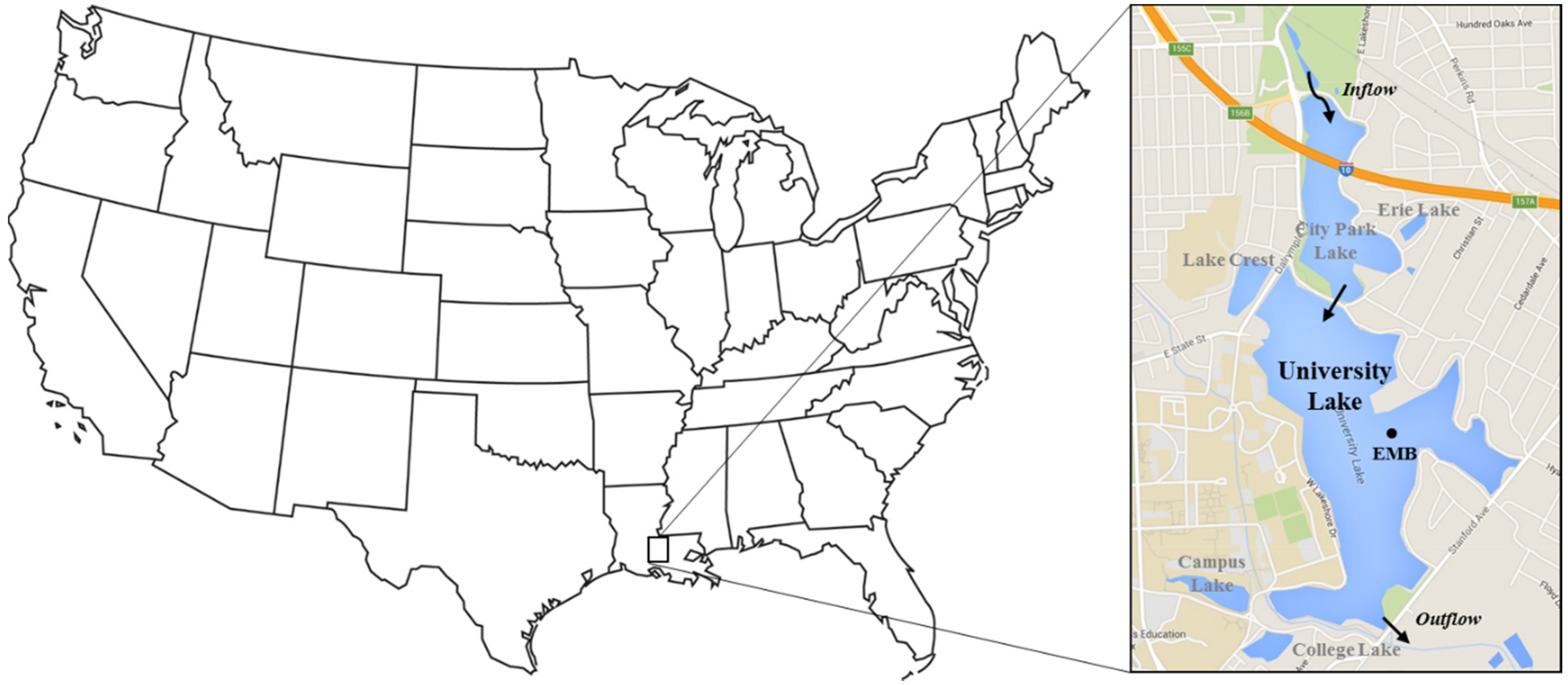
2.1. Site Description

The field observations were made at University Lake in Baton Rouge, South Louisiana, USA (Latitude 30°24’50″ N; Longitude 91°10’00″ W) on the Louisiana State University (LSU) campus (Figure 1). The lake has an open water surface of 74.6 ha with a perimeter of about 6.7 km and an average depth of 0.9 meter. The lake was artificially developed from a swamp area in the 1930s as a public works project to create an open water environment. The most recent dredging was conducted in 1983 when large amounts of sediments and excess nutrients from surface runoff were removed [29]. The drainage area of the entire lake watershed is about 187.4 ha [29,30] and land use of the watershed consists of residential, recreational, and institutional purposes. The lake is heavily affected by anthropogenic sources and a recent study found high concentrations of phosphorus [31] and chlorophyll-a [32].

Figure 1. Geographical location of University Lake in Baton Rouge, Louisiana, USA and the permanently deployed Environment Monitoring Buoy (EMB) in the lake.

Figure 1. Geographical location of University Lake in Baton Rouge, Louisiana, USA and the permanently deployed Environment Monitoring Buoy (EMB) in the lake.

South Louisiana has a humid-subtropical climate with long hot summers and short mild winters. Long-term annual temperature in the area was reported to be 20 °C, with monthly averages ranging from 11 °C in the coldest month (January) to 28 °C in the warmest month (July) [30]. The annual average air temperature during the 12 month study period (August 2008 to July 2009) recorded at Ben Hur weather station, which is about 5 km southeast of the study lake, was 20 °C, fluctuated from 10 °C in December 2008 to 26 °C in July 2009. During much of the 12-month study period, monthly average temperatures were lower than the long-term monthly averages. Long-term annual precipitation in the area was reported to be about 1477 mm, ranging from 159 mm in July to 81 mm in October [30]. Total precipitation during the 12-month study period was 1253 mm, ranging from a low monthly total of 11 mm in October 2008 to a high of 232 mm in September 2008.

2.2. Water Quality Monitoring

In the spring of 2008 an environment monitoring buoy (EMB) (YSI Inc., Yellow Springs, OH, USA) was deployed in the center of University Lake (Figure 1). The EMB was equipped with multi-probe data sondes (YSI 6920, Yellow Springs, OH, USA) that recorded dissolved oxygen at 15 min intervals at about 60 cm below the water surface. The sondes also measured a series of other water quality parameters including water temperature, pH, conductivity, turbidity, and chlorophyll-a concentration. During the study period from August 2008 to July 2009, the data sondes were calibrated monthly in laboratory.

2.3. Climatic Data Collection

Hourly climatic records were gathered for the study period from a nearby weather station (Ben Hur Station, the Louisiana Agriclimatic Information System) located approximately 5 km southeast of the study site. The records included a series of weather parameters, such as air temperature, precipitation, wind speed, humidity, solar radiation, and soil temperature. These data were used in the modeling for estimation of DO changes caused by photosynthesis and re-aeration, as described below.

3. Development of a Process-Based DO Model

Dissolved oxygen level in a water body is affected by production and consumption sources. This can be expressed in a balance equation as follows:

dDO/dt = P + J – R – S_SOD

(1)

where dDO/dt is the change in DO in mg O₂·L⁻¹·h⁻¹, P is the oxygen production by photosynthesis in mg O₂·L⁻¹·h⁻¹, J is the oxygen exchanging rate in mg O₂·L⁻¹·h⁻¹, R is the respiration rate in mg O₂·L⁻¹·h⁻¹, and S_SOD is the oxygen consumed by sediment oxygen demand in mg O₂·L⁻¹·h⁻¹. The estimation for the sources and sinks is described below.

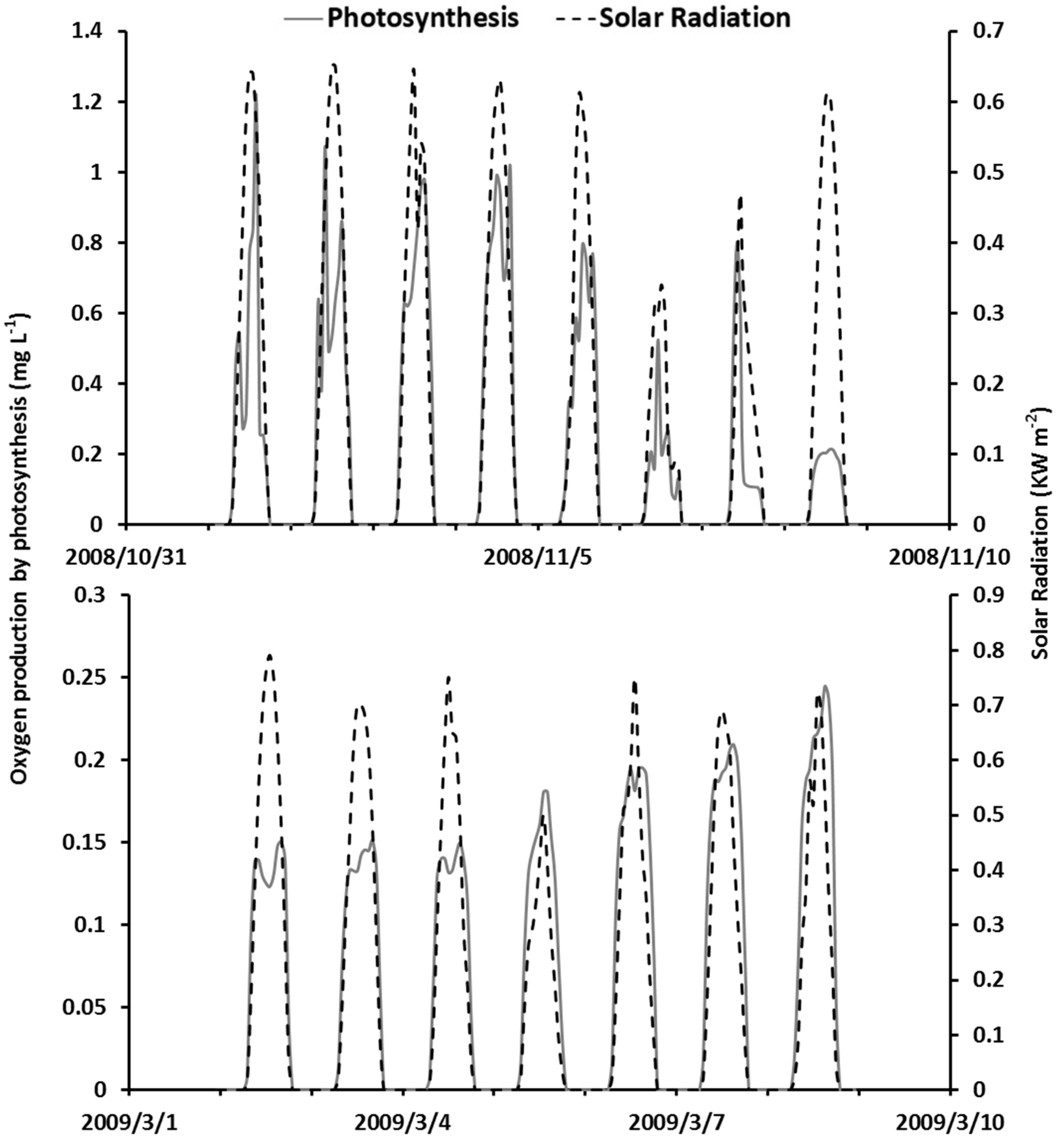
3.1. Oxygen Production by Photosynthesis

Photosynthesis is a process used by primary producers containing chlorophyll that releases free oxygen to the water body. It is affected by many factors including water temperature, intensity of photosynthetically active solar radiation (PAR), and dissolved nutrient concentration. In practice, photosynthesis is generally modeled as a function of light with a temperature correction factor [33]. In this model, photosynthesis is assumed to be a first-order kinetic process related with chlorophyll-a concentration. The formulation for oxygen production by photosynthesis is derived from Steele’s equation [34], represented by Bannister [35] and Culberson and Piedrahita [11]:

P = P_c × Chl-a

(2)

P_c = (α_par × R_s) × P_max × e^{(1−α_par × Rs)}

(3)

where P_c is the rate of chlorophyll-a dependent oxygen production in mg O₂·mg Chl-a⁻¹·h⁻¹, Chl-a is the chlorophyll-a concentration in mg·L⁻¹, R_s is the broadband solar radiation in kW·m⁻², and α_par is the ratio of PAR to broadband solar radiation in m²·kW⁻¹ for the studied region, which is often calculated as a constant ratio [36]. P_max is the maximum oxygen production rate by photosynthesis at saturating lighting conditions (mg O₂ (mg Chl-a × h)⁻¹). Chlorophyll-a concentration represents the biomass of phytoplankton in the lake and is depending on trophic status [37]. It could indirectly reflect dissolved nutrient concentrations. Therefore there is no variable in this equation for nutrient limitation.

P_max has been estimated as a temperature dependent variable and is consistent with the Arrhenius equation [38]:

P_max = 9.6 × 1.036^(T−20)

(4)

where T is water temperature in °C. Researchers [10] successfully applied it for inland lakes in north central United States.

Combining Equations (2)–(4), oxygen production through photosynthesis can be expressed as below:

P = (α_par × R_s) × [9.6 × 1.036^(T−20)] × e^{(1−α_par × Rs)} × Chl-a

(5)

3.2. Re-Aeration by Wind Regime

Re-aeration is another major oxygen source for water bodies. Water temperature can affect the capacity of dissolved oxygen saturation in a water body, while wind can accelerate oxygen dissolution. For lake systems, wind is considered to be the driving force in regulating surface turbulence, in contrast to the flow-induced turbulence that prevails in most streams [39]. Therefore, the equation for estimating physical re-aeration is derived from Gelda et al [39]:

J = α_j × (K_L/H) × (C_sat – C_s)

(6)

where α_j is the dimensionless re-aeration adjustment coefficient, K_L is the oxygen transfer coefficient in cm·h⁻¹, H is the thickness of the surface layer in cm and was set as a constant value of 60 in this study, C_sat is the saturated oxygen concentration in the surface layer at given temperature in mg O₂·L⁻¹, and C_s is the oxygen concentration in the water in mg O₂·L⁻¹.

The oxygen transfer coefficient is generally derived from either empirical or theoretical models [40]. To compute oxygen transfer coefficient, the equation discussed by Crusius and Wanninkhof [41] was used here for low wind speed over a lake, which is similar to the wind regime in the studied region:

For U < 3.7 m/s, K_L = 0.72U
For U ≥ 3.7 m/s, K_L = 4.33U – 13.3

(7)

where U is the hourly wind speed at 10 m height above the lake in m·s⁻¹ recorded by Ben Hur station of the Louisiana Agriclimatic Information System.

3.3. Respiration

Respiration is the reverse of photosynthesis, which consumes oxygen in the water. In this study, we assumed oxygen consumption by pelagic respiration is a first-order kinetics affected by external factors including water temperature and chlorophyll-a concentration. The equation derived from the study of Hull [15] was used as an approximation:

R = α_r × θ_r^(T−20) × Chl-a

(8)

where α_r is a respiration adjustment coefficient in h⁻¹, θ_r is the temperature adjustment coefficient, T is the hourly water temperature in °C, and Chl-a is the chlorophyll-a concentration in mg·L⁻¹. θ_r was reported as 1.045 by Ambrose and others [42] and successfully applied in some eutrophication models. In this study, the value of 1.045 was used for θ_r.

3.4. Sediment Oxygen Demand

Sediment (or benthic) oxygen demand (SOD) results from organic matter being deposited in the lakebed, which mainly depends on the temperature and the characteristics of the bed (physical, chemical and biological). The equation for SOD is given by Thomann and Mueller [43]:

S_SOD = S_S20 × θ_s^(T−20)/Z

(9)

where S_S20 is the sediment oxygen demand at 20°C in mg O₂·m⁻²·h⁻¹, Z is depth of the lake bottom sediment in meter, T is the water temperature in °C and θ_s is a temperature adjustment coefficient. In this study, Z was set as a constant of 1.2 meter based on field measurements and a value of 1.07 was used for θ_s according to previous studies [44].

3.5. Dissolved Oxygen Transport Equation

Combining the components, a one-dimensional DO model can be given as:

DO_v,t = DO_v,t-1 + (dDO_v/dt) × dt

(10)

where DO_v,t is DO concentration of V at time t in mg·L⁻¹, DO_v,t−1 is DO concentration of V at time t−1 in mg·L⁻¹, and dDO_v/dt is the rate of change in DO concentration in V during the time interval in mg·L⁻¹·h⁻¹, which is:

dDO_v/dt = (α_par × R_s) × [9.6 × 1.036^(T−20)] × e^{(1−α_par × Rs)} × Chl-a
+ α_j × (K_L/H) × (C_sat – C_s)
− α_r × θ_r^(T−20) × Chl-a
− S_S20 × θ_s^(T−20)/Z (11)

(11)

Equations (10) and (11) are for hourly dissolved oxygen dynamics. Chlorophyll-a concentration (Chl-a), water temperature (T), solar radiation (R_s) and wind speed (U) are model inputs, while adjustment coefficient for re-aeration (α_j) and respiration (α_r), the ratio of PAR to broadband solar radiation (α_par), and SOD (S_S20) are calibration coefficients. Other required coefficients and parameters are from literature review.

3.6. Model Limitations and Assumptions

Models may be more accurate if additional field data such as SOD were measured and used as model inputs. The choice of equations and coefficients from published literature were primarily based on the model performance with some considerations for the properties of the studied lake. For instance, the developed model is a one-dimensional model so water column is assumed to be well mixed because of its shallow depth.

3.7. DO Modeling

The model was calibrated and validated on an annual basis for the time period from August 2008 to July 2009. Means of 15-min records within an hour were used to represent hourly average. If more than two records in an hour were missing, data for that hour would be considered invalid. Only valid hourly data were used for calibration and validation. The studied time period was divided into four seasons, and each season—from spring to winter—was defined as a period of three continuous months with March being the first month of spring. Continuous valid hourly data for all four seasons were divided into two parts—one for calibration and the other for validation—and starting values were the first observed oxygen concentration. During the model run, if simulated DO was less than 0, the predicted DO for that time point was set to 0. The model was run for calibration until optimal fit was met between observations and simulations.

A sensitivity analysis to key parameters in the DO model was made after all the parameters and coefficients were fixed. Those fixed values were reference values for tested parameters in the sensitivity analysis. At a time only one parameter was changed from the reference value, and other coefficients were kept at the reference values. Parameters tested in the sensitivity analysis include the ratio of PAR to broadband solar radiation (α_par) and adjustment coefficient for re-aeration (α_j) and respiration (α_r), and SOD (S_S20). Results of sensitivity analysis were presented as changes rates of DO which were calculated by the following equation:

$$\mathsf{\Delta }\mathrm{DO}(\%)=\frac{{\sum }_{i=1}^n(\frac{D{O}_i^c-D{O}_i^b}{D{O}_i^b}\times 100)}{n}$$

(12)

where DO_i^c is i^th simulated DO value after one parameter was changed, DO_i^b is i^th baseline DO value estimated when the parameter was at the reference value, and n is the total number of observations in each tested period.

An uncertainty analysis was also taken to identify model parameter uncertainties. All calibrated parameters were tested in the uncertainty analysis during which only one parameter varies at a time while all the others remain fixed at calibrated values. Within a range of 50% and 150% of its calibrated value for each parameter, 6000 values were randomly selected for model runs to output 6000 sets of annual DO simulations. The means and standard deviations of 6000 annual average DO concentrations for each parameter were calculated and compared to the observed annual average DO concentration.

After calibration, sensitivity analysis and uncertainty analysis, the model was tested for validation.

3.8. Model Evaluation

Except graphical comparison between simulated DO and measured DO, coefficient of determination and Nash and Sutcliffe’s [45] model coefficient of efficiency (NSE) were used as the criteria evaluating model results. The coefficient of determination (R²) is defined as the squared value of Pearson’s correlation coefficient [46]. NSE is defined as:

$$\mathrm{NSE}=1-[\frac{{\sum }_{i=1}^n{\left(D{O}_i^{obs}-D{O}_i^{sim}\right)}^2}{{\sum }_{i=1}^n{\left(D{O}_i^{obs}-D{O}^{mean}\right)}^2}]$$

(13)

where DO_i^obs is the i^th DO observation for the time period being evaluated, DO_i^sim is the i^th simulated DO value for the interval being evaluated, DO^mean is the mean of observed DO for the constituent being evaluated, and n is the total number of observations.

Model runs for first 24 h were excluded from evaluation to avoid model spin-up effects. All the calculations were performed by SAS Statistical Software package (SAS Institute, Cary, NC, USA).

4. Results

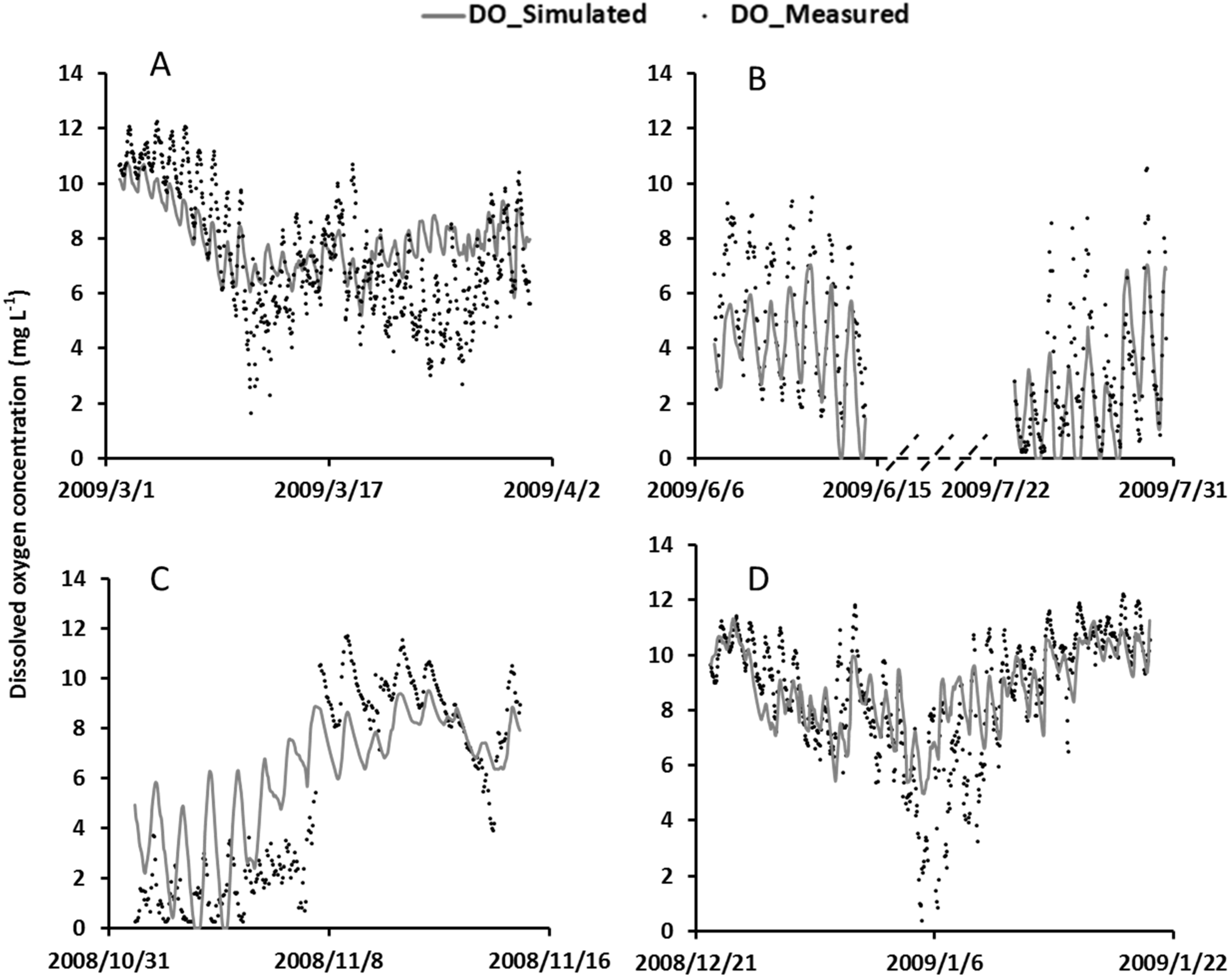
4.1. Model Calibration

Simulations showed good agreement between simulated DO and measured DO over the calibration period for all four seasons (Table 1). The rising/falling trends and the magnitude of peaks were well predicted for a variety of complex conditions, such as a period of hypoxia in late July, a sharp DO decrease in early November, and frequent highs and lows in spring and winter (Figure 2). In a few cases, the trend of DO dynamics was well reflected but magnitude was not strong enough (e.g., 5 January 2009, Figure 2). Hourly NSE for DO in calibration runs was 0.66 for the whole year and ranged from 0.41 to 0.58 for each season. R² was also 0.66 for the year and varied from 0.49 to 0.60 among seasons (Table 2). Both NSE and R² values appeared to be higher in the fall and winter (Table 2).

Table 1. Calibrated model parameters and parameter uncertainties. For each parameter in the uncertainty analysis, 6000 randomly chosen input values were passed through the model to obtain means and standard deviations (in italic) of the resulting annual average of DO concentrations.

Parameter	Calibrated Value	Uncertainty Analysis
		Value Range	Mean (Mg·L−1) ± Standard Deviation
αpar	2	[1,3]	6.40 ± 0.06
αj	2.6	[1.3,3.9]	6.33 ± 0.57
αr	7	[3.5,10.5]	6.53 ± 0.73
Ss20	0.083	[0.042,0.125]	6.45 ± 0.21

Table 1. Calibrated model parameters and parameter uncertainties. For each parameter in the uncertainty analysis, 6000 randomly chosen input values were passed through the model to obtain means and standard deviations (in italic) of the resulting annual average of DO concentrations.

Parameter	Calibrated Value	Uncertainty Analysis
		Value Range	Mean (Mg·L−1) ± Standard Deviation
αpar	2	[1,3]	6.40 ± 0.06
αj	2.6	[1.3,3.9]	6.33 ± 0.57
αr	7	[3.5,10.5]	6.53 ± 0.73
Ss20	0.083	[0.042,0.125]	6.45 ± 0.21

Table 2. Statistical results for calibration and validation of the deterministic DO model.

Month	Calibration			Validation
	n	r-Squared	NSE	n	r-Squared	NSE
Spring	707	0.49	0.41	1223	0.50	−0.42
Summer	365	0.60	0.48	177	0.59	0.46
Fall	332	0.61	0.57	384	0.42	0.32
Winter	708	0.60	0.58	822	0.51	−0.43
Year	2112	0.66	0.66	2606	0.61	0.21

Table 2. Statistical results for calibration and validation of the deterministic DO model.

Month	Calibration			Validation
	n	r-Squared	NSE	n	r-Squared	NSE
Spring	707	0.49	0.41	1223	0.50	−0.42
Summer	365	0.60	0.48	177	0.59	0.46
Fall	332	0.61	0.57	384	0.42	0.32
Winter	708	0.60	0.58	822	0.51	−0.43
Year	2112	0.66	0.66	2606	0.61	0.21

4.2. Uncertainty Analysis

The mean of 6000 average annual DO concentrations generated from a range of the parameters α_par, α_j, α_r and Ss₂₀ were 6.40, 6.33, 6.53 and 6.45 mg·L⁻¹, respectively (Table 1). These values were all close to the annual average (6.40 mg·L⁻¹) of observed DO concentrations with acceptable standard deviations. Specifically, αj had a relatively larger uncertainty compared with other parameters (Table 1).

4.3. Sensitivity Analysis

On an annual base the model was most sensitive to the coefficient of respiration (α_r) and re-aeration (α_j), less sensitive to the coefficient of SOD (S_S20), and least sensitive to the ratio of PAR to broadband solar radiation (α_par) (Table 3). Seasonally, the developed model was more sensitive to all parameters in summer and fall than in spring and winter. During cold months like spring and winter the model was almost equally sensitive to α_r and α_j, while in warm months like summer and fall α_r was the dominating parameter for model sensitivity. Throughout the studied year, the model sensitivity to Ss₂₀ was greater than α_par but less than α_r and α_j (Table 3).

Figure 2. Hourly simulation of dissolved oxygen concentration in model calibration for (A) spring; (B) summer (dashed line on x-axis means discontinuous time); (C) fall; and (D) winter.

Figure 2. Hourly simulation of dissolved oxygen concentration in model calibration for (A) spring; (B) summer (dashed line on x-axis means discontinuous time); (C) fall; and (D) winter.

Table 3. Results for sensitivity analysis.

Parameter a	Value	ΔDO (%)
		Year	Spring	Summer	Fall	Winter
αpar	3	−0.92	−0.13	−6.7	0.13	0.79
αpar	1	−5.2	−1.5	−12.7	−11.5	−2.1
αj	3.9	21.8	5.3	73.7	35.0	5.4
αj	1.3	−25.0	−15.1	−54.8	−36.1	−14.3
αr	10.5	−19.9	−8.9	−49.7	−30.3	−10.6
αr	3.5	62.9	8.9	216.7	120.2	10.6
Ss20	0.125	−7.7	−4.3	−22.6	−9.4	−2.7
Ss20	0.042	12.0	4.3	45.0	11.9	2.7

^a Reference values are fixed values after model calibration presented in Table 1.

Table 3. Results for sensitivity analysis.

Parameter a	Value	ΔDO (%)
		Year	Spring	Summer	Fall	Winter
αpar	3	−0.92	−0.13	−6.7	0.13	0.79
αpar	1	−5.2	−1.5	−12.7	−11.5	−2.1
αj	3.9	21.8	5.3	73.7	35.0	5.4
αj	1.3	−25.0	−15.1	−54.8	−36.1	−14.3
αr	10.5	−19.9	−8.9	−49.7	−30.3	−10.6
αr	3.5	62.9	8.9	216.7	120.2	10.6
Ss20	0.125	−7.7	−4.3	−22.6	−9.4	−2.7
Ss20	0.042	12.0	4.3	45.0	11.9	2.7

^a Reference values are fixed values after model calibration presented in Table 1.

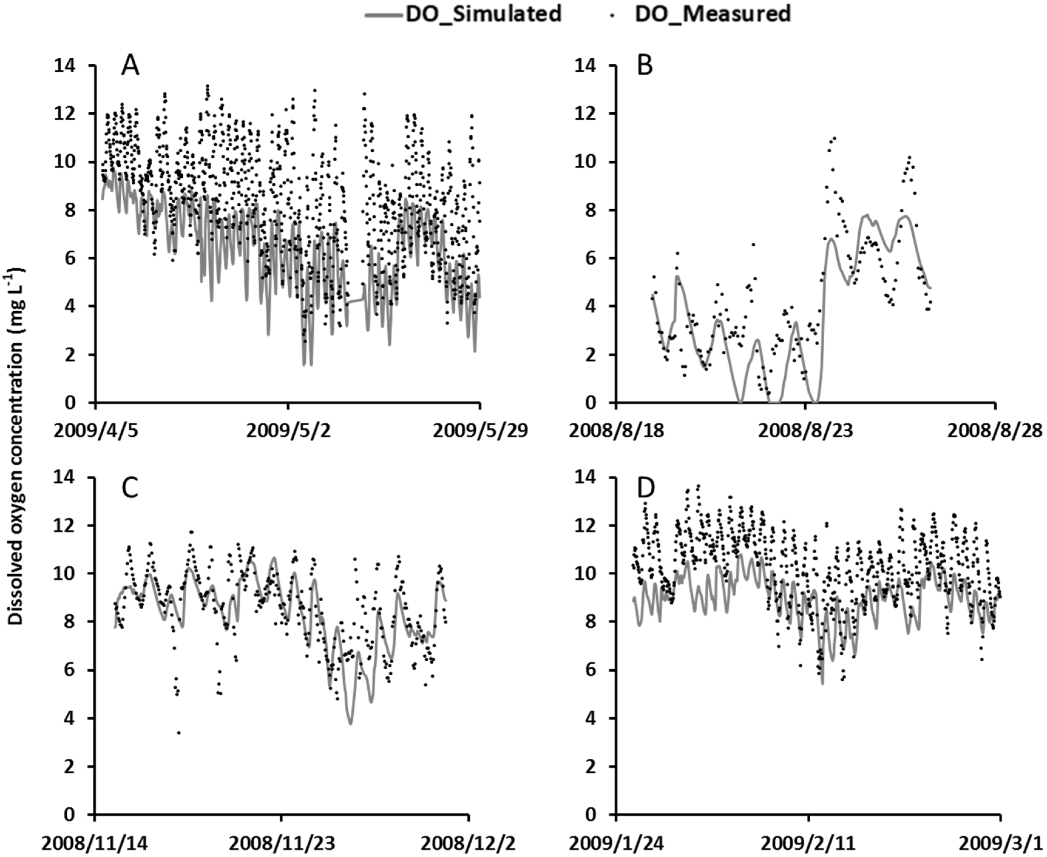
4.4. Model Validation

With the calibrated parameters, the DO model was applied to another continuous period in each calibrated season. Overall, the model produced satisfactory simulations for hourly DO change. Visual comparison showed agreement between the observed and simulated DO for most of the validation period, including the dramatic DO changes in early May and August. Simulated DO values were slightly underestimated in the spring and winter, although the moving trend was correctly predicted (Figure 3). Depending on the evaluation criteria, NSE and R² was 0.21 and 0.61 for the studied year, respectively (Table 2). Seasonally, from spring to winter, NSE was −0.42, 0.46, 0.32 and −0.43, respectively, and R² values were 0.50, 0.59, 0.42 and 0.51, respectively (Table 2).

Figure 3. Hourly simulation of dissolved oxygen concentration in model validation for (A) spring; (B) summer; (C) fall; and (D) winter.

Figure 3. Hourly simulation of dissolved oxygen concentration in model validation for (A) spring; (B) summer; (C) fall; and (D) winter.

4.5. The Interplay among Model Processes and Weather Conditions

As driving forces for the two dominant oxygen sources, effects of solar radiation and wind speed on photosynthesis and re-aeration can be further depicted in model output. In photosynthesis, hourly oxygen production went up and down along with the change of hourly solar radiation, but trends did not match well at daily peaks of irradiation (Figure 4). For the oxygen exchange at the air–water interface, wind contributed to transferring oxygen into the lake water when DO was under-saturated and out of the water when DO was oversaturated. Among all DO observations in summer and fall, about 15% were found oversaturated.

Figure 4. Comparison of hourly oxygen production by photosynthesis and intensity of solar radiation for selected days.

Figure 4. Comparison of hourly oxygen production by photosynthesis and intensity of solar radiation for selected days.

5. Discussions

5.1. Model Performance

Overall, the model showed a good prediction of diurnal DO trend over time. In previous water quality modeling studies, comparison of modeled results with observed records is mostly done at daily or monthly time intervals. Evaluation for hourly based modeling results using field measurements in water quality is very rare. We used both Nash and Sutcliffe’s [45] model coefficient of efficiency (NSE) and coefficient of determination for evaluation. Nash and Sutcliffe’s model coefficient of efficiency have been widely used to evaluate model performance for streamflow, surface runoff, sediments or nutrients [46], but most of published literature reported daily or monthly NSE [47]. Based on a monthly time step, NSE that is between 0.5 and 0.65 is considered as satisfactory, between 0.65 and 0.75 is taken as good, and equal or greater than 0.75 is rated as very good [47]. Coefficients of determination have been widely used as well, and typically values of R² greater than 0.5 are considered acceptable for models on a daily or monthly time step [47,48,49]. Due to the fact that averaging values significantly decreases the variation, models with higher frequency were always reported with lower NSE and R² [50,51,52,53]. Some researchers [49,54] reported NSE values between 0.36 to 0.75 as satisfactory and greater than 0.75 as good on a daily time step. Therefore, based on our results, we propose to consider an NSE value of less than 0.30 as unsatisfactory, an NSE value between 0.30 to 0.60 as satisfactory, and an NSE value of greater than 0.60 as good for DO modeling at an hourly resolution. Similarly, for the coefficient of determination, values of R² equal or greater than 0.45 and 0.65 can be considered acceptable and good, respectively, for high frequency DO modeling. In this case, evaluated either by coefficient of determination or NSE, the majority of model outputs are satisfactory and good. Specifically, the developed model performed well for simulating dramatic DO drops within a day for most cases. In a model with a lower frequency (i.e., daily), a rapid change in DO during the day cannot be well reflected when data are averaged.

The sensitivity of the DO model to key parameters in the studied lake is very different when compared to models developed for deep lakes or reservoirs. A previous study [10] showed that in deep lakes, simulated epilimnetic dissolved oxygen is insensitive to nearly all model coefficients because of strong mixing and surface re-aeration, and hypolimnetic DO is very sensitive to SOD but not to photosynthesis and attenuation [10]. In this studied lake which is shallow and eutrophic, even with strong internal mixing and surface re-aeration, the model still seems to be very sensitive to respiration. When biological activities of phytoplankton are inhibited, the model is then most sensitive to re-aeration. SOD is important much of the time, but is not the most significant throughout the year. This condition may also apply for other lakes of a similar type.

Common productivity analyses use respiration measurements made at night as a constant to estimate respiration during the day [55]. Compared to that, the use of chlorophyll-a as a surrogate in this study for pelagic phytoplankton biomass has generated better simulation results. This may have resulted from the long eutrophic conditions present in the studied lake during the most of a year [31,32]. Previous researchers have found that respiration and chlorophyll-a concentration closely and positively correlated with chlorophyll-a levels in excess of 5 µg·L⁻¹ [56,57]. Iriarte et al argued that heterotrophs could make the most substantial contribution to community respiration rates at low and moderate chlorophyll-a concentrations, while under conditions of exceptionally high phytoplankton biomass, autotrophic dark respiration could be the dominant component of plankton community respiration in the water column [56]. Based on Carlson’s trophic state index, eutrophic waters have high concentrations of chlorophyll-a (≥20 µg·L⁻¹), so the microalgae would dominate the plankton community respiration rates most of the time. In this case, the use of chlorophyll-a for the estimation of pelagic respiration could be feasible for most eutrophic waters, especially for those in tropical and subtropical regions whose winters are relatively short and mild. In colder regions, phytoplankton could die off in the winter and early spring due to a drastic temperature drop; therefore seasonality should be considered if chlorophyll-a is used for respiration simulation. Furthermore, respiration may be better estimated if we could separate autotrophic from heterotrophic respiration [33]. In this present study, the lack of individual heterotrophic respiration measurements could be a reason why the sensitivity of α_r is relatively low during winter and spring and why there is a general discrepancy for these seasons in validation. However, due to the limitation of data availability, heterotrophic respiration is not added to the model in this study. Further study is needed to test the significance of heterotrophic respiration in DO modeling.

5.2. Dynamic Interplay among Model Processes and Weather Conditions

The lack of knowledge for the dynamic interactions among model processes and weather conditions could be a reason for the discrepancies in model simulation. One instance is the relationship between solar radiation and photosynthesis, which is not clearly understood, especially in a high frequency model. The mismatching between photosynthesis and solar radiation during the hours of maximum irradiation could be attributed to photoinhibition. Photoinhibition is negative to the efficiency of photosynthesis, the strength of which is directly proportional to light intensity [58]. The effects of photoinhibition would cause a marked slow-down for photosynthesis at daily peaks of irradiation, but are always ignored in models with lower frequency. In this study, obvious slow-downs in photosynthesis could be found in some model simulations (e.g., early March in 2009, Figure 4) but in not all of them, and the degree of the slow-down in photosynthesis is overestimated sometime (e.g., early November in 2009, Figure 4). This indicates that the addition of photoinhibition as a component of photosynthesis could be beneficial for DO models with high frequency, especially for eutrophic water bodies.

Another alternative explanation for the variation of photosynthetic production in the middle of the day is photorespiration. Photorespiration occurs in the photosynthetic tissues and is completely distinct from ordinary respiration, which is essentially mitochondrial [15,59]. It is enhanced with increased temperature and oxygen concentration and decreased carbon dioxide concentration [60]. Previous studies have reported that 10% to 25% of oxygen production by photosynthesis could be consumed because of photorespiration [11,60]. Field and laboratory experiments in a shallow lake in Italy also shows that primary production slowed down obviously at the peak of solar radiation due to photorespiration, especially in spring and summer [15]. The photorespiration processes is also neglected in most of DO models since they can only be directly observed in models with high frequency. In DO modeling, photorespiration could be estimated based on photosynthetic production or respiration. Successful trials for that include Culberson and Piedrahita’s study [11] in which an individual equation for photorespiration was added in the primary production in their DO model for an aquaculture pond and successful simulations were yielded. Moreover, Parkhill and Gulliver added photorespiration to their whole-stream respiration model and proved that accounting for photorespiration in the streams could increase the apparent efficiency of photosynthesis, improve the accuracy of DO predictions, and reduce uncertainty in photosynthesis and respiratory rate estimates [61]. Similar to photoinhibition, photorespiration could be taken into consideration for an improved estimation of photosynthetic production as well. In addition, one of the existing concerns for the application of photorespiration in DO modeling is the fact that photorespiration could not be consistently observed when the system has very low productivity [61]. This indicates that the use of photorespiration would be more important and applicable for eutrophic waters. In addition, significant photorespiration is not perceptible if the duration of light that affects the primary producers is very short [62]. So some applications may not be able to reduce predictive errors by accounting for the effect of light on respiratory rates under certain weather conditions (e.g., constant cloudiness).

6. Conclusions

This study developed an hourly deterministic model of dissolved oxygen and applied the model to a subtropical eutrophic shallow lake for a one-year period. The model incorporated important source and sink components of dissolved oxygen for a lake system, such as photosynthesis, re-aeration, pelagic respiration, and sediment oxygen demand. Overall, the model produced satisfactory results, providing a modeling approach for predicting potential effects of rapid, sporadic hypoxic events on DO. However, a knowledge gap still exists in accurately quantifying oxygen produced by photosynthesis in high frequency DO modeling.

References

1. Frodge, J.D.; Thomas, G.L.; Pauley, G.B. Effects of canopy formation by floating and submergent aquatic macrophytes on the water-quality of 2 shallow pacific-northwest lakes. Aquat. Bot. 1990, 38, 231–248. [Google Scholar] [CrossRef]
2. Diaz, R.J.; Rosenberg, R. Spreading dead zones and consequences for marine ecosystems. Science 2008, 321, 926–929. [Google Scholar] [CrossRef] [PubMed]
3. Kemp, W.M.; Sampou, P.; Caffrey, J.; Mayer, M.; Henriksen, K.; Boynton, W.R. Ammonium recycling versus denitrification in chesapeake bay sediments. Limnol. Oceanogr. 1990, 35, 1545–1563. [Google Scholar] [CrossRef]
4. Breitburg, D.L. Episodic hyp oxia in Chesapeake Bay—Interacting effects of recruitment, behavior, and physical disturbance. Ecol. Monographs 1992, 62, 525–546. [Google Scholar] [CrossRef]
5. Hamilton, S.K.; Sippel, S.J.; Calheiros, D.F.; Melack, J.M. An anoxic event and other biogeochemical effects of the pantanal wetland on the Paraguay River. Limnol. Oceanogr. 1997, 42, 257–272. [Google Scholar] [CrossRef]
6. Gray, J.S.; Wu, R.S.S.; Or, Y.Y. Effects of hypoxia and organic enrichment on the coastal marine environment. Mar. Ecol. Prog. Ser. 2002, 238, 249–279. [Google Scholar] [CrossRef]
7. Harrison, J.A.; Matson, P.A.; Fendorf, S.E. Effects of a diel oxygen cycle on nitrogen transformations and greenhouse gas emissions in a eutrophied subtropical stream. Aquat. Sci. 2005, 67, 308–315. [Google Scholar] [CrossRef]
8. Stevens, P.W.; Blewett, D.A.; Casey, J.P. Short-term effects of a low dissolved oxygen event on estuarine fish assemblages following the passage of hurricane charley. Estuar. Coasts 2006, 29, 997–1003. [Google Scholar] [CrossRef]
9. Holtgrieve, G.W.; Schindler, D.E.; Jankowski, K. Comment on Demars et al. 2015, “Stream metabolism and the open diel oxygen method: Principles, practice, and perspectives”. Limnol. Oceanogr. Methods 2015. [Google Scholar] [CrossRef]
10. Stefan, H.G.; Fang, X. Dissolved-oxygen model for regional lake analysis. Ecol. Model. 1994, 71, 37–68. [Google Scholar] [CrossRef]
11. Culberson, S.D.; Piedrahita, R.H. Aquaculture pond ecosystem model: Temperature and dissolved oxygen prediction—Mechanism and application. Ecol. Model. 1996, 89, 231–258. [Google Scholar] [CrossRef]
12. Haider, H.; Ali, W.; Haydar, S. Evaluation of various relationships of reaeration rate coefficient for modeling dissolved oxygen in a river with extreme flow variations in Pakistan. Hydrol. Process. 2013, 27, 3949–3963. [Google Scholar] [CrossRef]
13. Benson, A.; Zane, M.; Becker, T.E.; Visser, A.; Uriostegui, S.H.; DeRubeis, E.; Moran, J.E.; Esser, B.K.; Clark, J.F. Quantifying reaeration rates in alpine streams using deliberate gas tracer experiments. Water 2014, 6, 1013–1027. [Google Scholar]
14. Haider, H.; Ali, W. Calibration and verification of a dissolved oxygen management model for a highly polluted river with extreme flow variations in Pakistan. Environ. Monit. Assess. 2013, 185, 4231–4244. [Google Scholar]
15. Hull, V.; Parrella, L.; Falcucci, M. Modelling dissolved oxygen dynamics in coastal lagoons. Ecol. Model. 2008, 211, 468–480. [Google Scholar] [CrossRef]
16. Rucinski, D.K.; Beletsky, D.; DePinto, J.V.; Schwab, D.J.; Scavia, D. A simple 1-dimensional, climate based dissolved oxygen model for the central basin of Lake Erie. J. Great Lakes Res. 2010, 36, 465–476. [Google Scholar] [CrossRef]
17. Benoit, P.; Gratton, Y.; Mucci, A. Modeling of dissolved oxygen levels in the bottom waters of the lower St. Lawrence estuary: Coupling of benthic and pelagic processes. Mar. Chem. 2006, 102, 13–32. [Google Scholar] [CrossRef]
18. Mooij, W.M.; Trolle, D.; Jeppesen, E.; Arhonditsis, G.; Belolipetsky, P.V.; Chitamwebwa, D.B.R.; Degermendzhy, A.G.; DeAngelis, D.L.; Domis, L.N.D.; Downing, A.S.; et al. Challenges and opportunities for integrating lake ecosystem modelling approaches. Aquat. Ecol. 2010, 44, 633–667. [Google Scholar] [CrossRef] [Green Version]
19. James, R.T.; Martin, J.; Wool, T.; Wang, P.F. A sediment resuspension and water quality model of Lake Okeechobee. J. Am. Water Resour. Assoc. 1997, 33, 661–680. [Google Scholar] [CrossRef]
20. Tundisi, J.G. Perspectives for ecological modeling of tropical and subtropical reservoirs in South-America. Ecol. Model. 1990, 52, 7–20. [Google Scholar] [CrossRef]
21. D’Autilia, R.; Falcucci, M.; Hull, V.; Parrella, L. Short time dissolved oxygen dynamics in shallow water ecosystems. Ecol. Model. 2004, 179, 297–306. [Google Scholar] [CrossRef]
22. Oren, A. Saltern evaporation ponds as model systems for the study of primary production processes under hypersaline conditions. Aquat. Microbial Ecol. 2009, 56, 193–204. [Google Scholar] [CrossRef]
23. Wan, Y.S.; Ji, Z.G.; Shen, J.; Hu, G.D.; Sun, D.T. Three dimensional water quality modeling of a shallow subtropical estuary. Mar. Environ. Res. 2012, 82, 76–86. [Google Scholar] [CrossRef] [PubMed]
24. Blauw, A.N.; Los, H.F.J.; Bokhorst, M.; Erftemeijer, P.L.A. Gem: A generic ecological model for estuaries and coastal waters. Hydrobiologia 2009, 618, 175–198. [Google Scholar] [CrossRef]
25. Pena, M.A.; Katsev, S.; Oguz, T.; Gilbert, D. Modeling dissolved oxygen dynamics and hypoxia. Biogeosciences 2010, 7, 933–957. [Google Scholar] [CrossRef]
26. Rabalais, N.N.; Turner, R.E.; Wiseman, W.J. Hypoxia in the Gulf of Mexico. J. Environ. Qual. 2001, 30, 320–329. [Google Scholar] [CrossRef] [PubMed]
27. Yin, K.D.; Lin, Z.F.; Ke, Z.Y. Temporal and spatial distribution of dissolved oxygen in the Pearl River estuary and adjacent coastal waters. Cont. Shelf Res. 2004, 24, 1935–1948. [Google Scholar] [CrossRef]
28. Xu, Z.; Xu, Y.J. Determination of trophic state changes with diel dissolved oxygen: A case study in a shallow lake. Water Environ. Res. 2015, 87, 1970–1979. [Google Scholar] [CrossRef] [PubMed]
29. Reich Association. City Park/University Lakes Management Plan; Applied Technology Research Corporation: Baton Rouge, LA, USA, 1991. [Google Scholar]
30. Xu, Y.J.; Mesmer, R. The dynamics of dissolved oxygen and metabolic rates in a shallow subtropical urban lake, Louisiana, USA. In Understanding Freshwater Quality Problems in a Changing World; Berit, A., Ed.; International Association of Hydrological Sciences (IAHS): Wallingford, UK, 2013; pp. 212–219. [Google Scholar]
31. Mesmer, R. Impact of Urban Runoff of Phosphorus, Nitrogen and Dissolved Oxygen in a Shallow Subtropical Lake. Master’s Thesis, Louisiana State University and Agricultural and Mechanical College, Raton Rouge, LA, USA, 2010. [Google Scholar]
32. Xu, Z.; Xu, Y.J. Rapid field estimation of biochemical oxygen demand in a subtropical eutrophic urban lake with chlorophyll a fluorescence. Environ. Monit. Assess. 2015, 187, 14. [Google Scholar] [CrossRef] [PubMed]
33. Demars, B.O.L.; Thompson, J.; Manson, J.R. Stream metabolism and the open diel oxygen method: Principles, practice, and perspectives. Limnol. Oceanogr. Methods 2015, 13, 356–374. [Google Scholar] [CrossRef]
34. Steele, J.H. Environmental control of photosynthesis in the sea. Limnol. Oceanogr. 1962, 7, 137–150. [Google Scholar] [CrossRef]
35. Banniste, T.T. Production equations in terms of chlorophyll concentration, quantum yield, and upper limit to production. Limnol. Oceanogr. 1974, 19, 1–12. [Google Scholar] [CrossRef]
36. Alados, I.; FoyoMoreno, I.; AladosArboledas, L. Photosynthetically active radiation: Measurements and modelling. Agric. Forest Meteorol. 1996, 78, 121–131. [Google Scholar] [CrossRef]
37. Gregor, J.; Marsalek, B. Freshwater phytoplankton quantification by chlorophyll α: A comparative study of in vitro, in vivo and in situ methods. Water Res. 2004, 38, 517–522. [Google Scholar] [CrossRef] [PubMed]
38. Megard, R.O.; Tonkyn, D.W.; Senft, W.H. Kinetics of oxygenic photosynthesis in planktonic algae. J. Plankton Res. 1984, 6, 325–337. [Google Scholar] [CrossRef]
39. Gelda, R.K.; Auer, M.T.; Effler, S.W.; Chapra, S.C.; Storey, M.L. Determination of reaeration coefficients: Whole-lake approach. J. Environ. Eng. 1996, 122, 269–275. [Google Scholar] [CrossRef]
40. Demars, B.O.L.; Manson, J.R. Temperature dependence of stream aeraion coefficients and the effect of water turbulence: A critival review. Water Res. 2013, 47, 1–15. [Google Scholar] [CrossRef] [PubMed]
41. Crusius, J.; Wanninkhof, R. Gas transfer velocities measured at low wind speed over a lake. Limnol. Oceanogr. 2003, 48, 1010–1017. [Google Scholar] [CrossRef]
42. Ambrose, R.B.; Wool, T.A.; Connolly, J.P.; Schanz, R.W. WASP4 (EUTRO4), A Hydrodynamic and Water Quality Model—Model Theory, User′s Manual, and Programmer′s Guide; EPA/600/3–87/039; U.S. Environmental Protection Agency: Athens, GA, USA, 1988.
43. Thomann, R.V.; Mueller, J.A. Principles of Surface Water Quality Modeling and Control; Harper & Row: New York, NY, USA, 1987. [Google Scholar]
44. Zison, S.W.; Mills, W.B.; Diemer, D.; Chen, C.W. Rates, Constants and Kinetic Formulations in Surface Water Quality Modeling; EPA 600-3-78-105; Tetra Tech., Inc. for U.S. Environmental Protection Agency: Athens, GA, USA, 1978.
45. Nash, J.E.; Sutcliffe, J.E. River flow forecasting through conceptual models, Part I—A discussion of principles. J. Hydrol. 1970, 10, 282–290. [Google Scholar] [CrossRef]
46. Legates, D.R.; McCabe, G.J. Evaluating the use of “goodness-of-fit” measures in hydrologic and hydroclimatic model validation. Water Resour. Res. 1999, 35, 233–241. [Google Scholar] [CrossRef]
47. Moriasi, D.N.; Arnold, J.G.; van Liew, M.W.; Bingner, R.L.; Harmel, R.D.; Veith, T.L. Model evaluation guidelines for systematic quantification of accuracy in watershed simulations. Trans. ASABE 2007, 50, 885–900. [Google Scholar] [CrossRef]
48. Santhi, C.; Arnold, J.G.; Williams, J.R.; Dugas, W.A.; Srinivasan, R.; Hauck, L.M. Validation of the swat model on a large river basin with point and nonpoint sources. J. Am. Water Resour. Assoc. 2001, 37, 1169–1188. [Google Scholar] [CrossRef]
49. Van Liew, M.W.; Arnold, J.G.; Garbrecht, J.D. Hydrologic simulation on agricultural watersheds: Choosing between two models. Trans. ASAE 2003, 46, 1539–1551. [Google Scholar] [CrossRef]
50. Fernandez, G.P.; Chescheir, G.M.; Skaggs, R.W.; Amatya, D.M. Development and testing of watershed-scale models for poorly drained soils. Trans. ASAE 2005, 48, 639–652. [Google Scholar] [CrossRef]
51. Singh, J.; Knapp, H.V.; Arnold, J.G.; Demissie, M. Hydrological modeling of the Iroquois River watershed using HSPF and SWAT. J. Am. Water Resour. Assoc. 2005, 41, 343–360. [Google Scholar] [CrossRef]
52. Wu, K.; Xu, Y.J. Evaluation of the applicability of the swat model for coastal watersheds in southeastern Louisiana. J. Am. Water Resour. Assoc. 2006, 42, 1247–1260. [Google Scholar] [CrossRef]
53. Van Liew, M.W.; Veith, T.L.; Bosch, D.D.; Arnold, J.G. Suitability of swat for the conservation effects assessment project: Comparison on USDA agricultural research service watersheds. J. Hydrol. Eng. 2007, 12, 173–189. [Google Scholar] [CrossRef]
54. Motovilov, Y.G.; Gottschalk, L.; Engeland, K.; Rodhe, A. Validation of a distributed hydrological model against spatial observations. Agric. Forest Meteorol. 1999, 98–99, 257–277. [Google Scholar] [CrossRef]
55. Portielje, R.; Kersting, K.; Lijklema, L. Primary production estimation from continuous oxygen measurements in relation to external nutrient input. Water Res. 1996, 30, 625–643. [Google Scholar] [CrossRef]
56. Iriarte, A.; Daneri, G.; Garcia, V.M.T.; Purdie, D.A.; Crawford, D.W. Plankton community respiration and its relationship to chlorophyll a concentration in marine coastal waters. Oceanol. Acta 1991, 14, 379–388. [Google Scholar]
57. Fourqurean, J.W.; Webb, K.L.; Hollibaugh, J.T.; Smith, S.V. Contributions of the plankton community to ecosystem respiration, Tomales Bay, California. Estuar. Coast. Shelf Sci. 1997, 44, 493–505. [Google Scholar] [CrossRef]
58. Tyystjarvi, E.; Aro, E.M. The rate constant of photoinhibition, measured in lincomycin-treated leaves, is directly proportional to light intensity. Proc. Natl. Acad. Sci. USA 1996, 93, 2213–2218. [Google Scholar] [CrossRef] [PubMed]
59. Beardall, J. Photosynthesis and photorespiration in marine-phytoplankton. Aquat. Bot. 1989, 34, 105–130. [Google Scholar] [CrossRef]
60. Sharkey, T.D. Estimating the rate of photorespiration in leaves. Physiol. Plant. 1988, 73, 147–152. [Google Scholar] [CrossRef]
61. Parkhill, K.L.; Gulliver, J.S. Application of photorespiration concepts to whole stream productivity. Hydrobiologia 1998, 389, 7–19. [Google Scholar] [CrossRef]
62. Parkhill, K.L.; Gulliver, J.S. Modeling the effect of light on whole-stream respiration. Ecol. Model. 1999, 117, 333–342. [Google Scholar] [CrossRef]