Modeling Climate and Management Change Impacts on Water Quality and In-Stream Processes in the Elbe River Basin

Hesse, Cornelia; Krysanova, Valentina

doi:10.3390/w8020040

Open AccessArticle

Modeling Climate and Management Change Impacts on Water Quality and In-Stream Processes in the Elbe River Basin

by

Cornelia Hesse

^* and

Valentina Krysanova

Potsdam-Institute for Climate Impact Research, Post Box 601203, Potsdam 14412, Germany

^*

Author to whom correspondence should be addressed.

Water 2016, 8(2), 40; https://doi.org/10.3390/w8020040

Submission received: 14 September 2015 / Revised: 12 January 2016 / Accepted: 25 January 2016 / Published: 28 January 2016

(This article belongs to the Special Issue Water Resource Variability and Climate Change)

Download

Browse Figures

Versions Notes

Abstract

:

Eco-hydrological water quality modeling for integrated water resources management of river basins should include all necessary landscape and in-stream nutrient processes as well as possible changes in boundary conditions and driving forces for nutrient behavior in watersheds. The study aims to assess possible impacts of the changing climate (ENSEMBLES climate scenarios) and/or land use conditions on resulting river water quantity and quality in the large-scale Elbe river basin by applying a semi-distributed watershed model of intermediate complexity (SWIM) with implemented in-stream nutrient (N+P) turnover and algal growth processes. The calibration and validation results revealed the ability of SWIM to satisfactorily simulate nutrient behavior at the watershed scale. Analysis of 19 climate scenarios for the whole Elbe river basin showed a projected increase in temperature (+3 °C) and precipitation (+57 mm) on average until the end of the century, causing diverse changes in river discharge (+20%), nutrient loads (NO₃-N: −5%; NH₄-N: −24%; PO₄-P: +5%), phytoplankton biomass (−4%) and dissolved oxygen concentration (−5%) in the watershed. In addition, some changes in land use and nutrient management were tested in order to reduce nutrient emissions to the river network.

Keywords:

Elbe river basin; water quality modeling; in-stream processes; nutrients; SWIM; climate change impact assessment; ENSEMBLES; management change impacts

1. Introduction

Changes of the world’s and Europe’s climate and increased anthropogenic pressure on natural resources have already been detected in the past, and this development is likely to continue in the future [1,2,3,4,5,6].

Looking at the climate aspect, a global rise in mean temperature, change in precipitation pattern as well as an increase in intensity and frequency of extreme events can be recognized [1,2,7], impacting the water cycle [8,9,10], vegetation and biodiversity [11,12,13,14] as well as human health [15,16] and economy [17,18]. The potential warming in Europe could reach values from +1 to +6 °C by the end of this century [19], depending on the location. The annual mean precipitation is expected to increase in Northern Europe and decrease in most parts of Southern Europe and Mediterranean regions up to ±20% [20]. The catchment of the Elbe river, mainly located in Germany and the Czech Republic in Central Europe, is already experiencing changes in climate conditions as well as changes in extreme temperature and precipitation values, and this trend is expected to continue. During the last century (1882–2013) the average temperature in Germany increased by 1.2 °C, whereas the precipitation amounts rose by 10.6% on average with a high spatial and temporal variability [21]. Application of ensembles of climate scenarios shows increasing trends in floods for the Elbe basin in Germany [22] as well as in the Czech Republic [23], especially in wintertime.

Climate change will have direct and indirect impacts on river water quantity and quality [24,25,26,27,28]. With the rising temperature, water availability will decrease due to increased evapotranspiration, and a reduced discharge will facilitate algal growth and reduce dilution of point source pollutants. Higher temperatures and lower flow velocities would additionally stimulate turnover processes and increase system respiration rates, causing oxygen deficits in river reaches. All these processes lead to the degradation of water quality and ecological status of a waterbody connected with a higher probability of algal blooms [24,29,30] and increasing problems for water supply and treatment [25].

As phytoplankton growth is a key factor for water quality in lowland river ecosystems [31], the algal processes should be included in evaluating impacts of global change on water quality. Light and nutrients are generally deemed to be the most important external drivers of phytoplankton dynamics in rivers, along with temperature which also has a positive relationship with phytoplankton, and discharge which has a negative relationship [29,30,31].

Additionally, climate change would influence nutrient turnover and transport processes (denitrification, nitrification, volatilization and leaching) in the catchments, due to altered temperature and precipitation [32,33,34], and the terrestrial processes will also influence the final river water quality at the outlet of the basin. River systems are also affected by anthropogenic impacts (land use composition, population and industry) causing nutrient pollution from point (factories, sewage treatment plants) and diffuse sources (agricultural fields), which lead to eutrophication processes and a decrease in river water quality [35,36,37,38].

Due to the high pressure of rising population, growing industry and increasing transport demand on landscapes and natural vegetation, many changes in land use could be recognized in Europe in the past. The current tendencies include a decreasing trend in crop and pasture acreages in Spain, Czech Republic and Northern Germany, slowly growing forested areas in Northern Europe and Portugal, and notably growing urban areas in France and Western Germany [5,39]. It is expected that these trends will continue in the coming 10–20 years.

Population density and human activities are important underlying factors for point and diffuse nutrient pollution entering rivers [40]. During the last decades, many efforts to reduce nutrient inputs to the rivers by construction and improvement of sewage treatment plants and optimization of fertilizer application on cropland were undertaken in Europe. They resulted in a remarkable reduction of phosphorus emissions (mainly from point sources), but only a small decrease of nitrogen inputs (mainly from diffuse sources) due to the lag time of diffuse nutrients in soils [41,42,43]. It is widely recognized that the control of diffuse source emissions is much more difficult. So it is expected that the inputs of nutrients from households and industry will be further reduced in the future, and diffuse inputs from fertilizers and manure will become the main sources of nutrient pollution in Europe [42].

Climate as well as land use change impacts on river water quality superimpose each other and create a very complex system of interactions and feedbacks [27,44,45]. The nitrate loads in the rivers, for example, are climate-dependent, and were likely influenced by former climate variations, so it is difficult to define and interpret the pure effects of management changes in the past [41]. Furthermore, adaptation measures and policy responses to projected climate change, e.g., subvention for bio-fuels or control of greenhouse gas emissions, affect freshwater quality as well [24]. A combined land use and climate change impact assessment would be an important step facilitating an integrated river basin management. The system characteristics and variable boundary conditions should be taken into account by default in modern management strategies [31] to support the implementation of adaptation measures in river basins.

The process-based eco-hydrological watershed models driven by climate and land use parameters can be useful for assessing potential future developments in a changing world. Watershed models including both landscape and in-stream nutrient processes, which are able to simulate nutrient turnover processes in a catchment and river network, may represent effective tools for the evaluation of river water quality at the basin scale [46,47]. However, it should be kept in mind that current water quality modeling at the watershed scale still has more weaknesses and uncertainties compared to pure hydrological modeling due to the higher complexity of modeled processes and the requirement to include more input data and parameters.

In former applications of the semi-distributed eco-hydrological Soil and Water Integrated Model (SWIM) [48] for water quality modeling in river basins in Germany, it was observed that nutrient retention and decomposition solely in the soils of the watershed is not sufficient for tackling nutrients coming from different sources, especially in larger basins [49]. Therefore, SWIM was extended by a new module representing nutrient and oxygen turnover processes and algal growth in rivers, which was already tested for the mesoscale Saale river, a sub-catchment of the Elbe river with an area of about 25,000 km² [50]. The aim of this study is to apply the new SWIM version for a combined climate and land use change impact assessment on the entire Elbe basin including the upstream part in the Czech Republic and the lower part in Germany (total drainage area about 150,000 km²). This can support the development of management strategies and adaptation measures to potential changes in the future in this large-scale river basin.

In particular, the following objectives were pursued in this study:

Testing the in-stream SWIM module for the large scale by modeling water quality parameters (nitrate nitrogen (NO₃-N), ammonium nitrogen (NH₄-N), phosphate phosphorus (PO₄-P), dissolved oxygen (DOX), and chlorophyll a (Chla)) at the basin outlet and at confluences of the large Elbe tributaries in the historical period;
Analysis of climate scenarios for the region provided by the European ENSEMBLES project [51], and climate change impact assessment on water quantity and quality for two future periods (2021–2050 and 2071–2100) with unchanged management;
Simulation of selected land use change and management scenarios aiming at the reduction of point and diffuse nutrient loads in the basin; and
Analysis of the combined climate and land use change impacts on water quantity and quality to derive ideas for suitable measures for adaptation to climate change.

The model-based assessments of climate and land use change impacts on water quality are rare in literature so far compared to impact assessments on the hydrological cycle, especially at the large scale. The recently implemented in-stream module enables a more realistic representation of all interrelated processes for the impact study. Therefore, this study is an important step forward to large-scale application of water quality models with distributed calibration for impact studies in general, as well as towards a fully integrated water resources assessment in the Elbe catchment in particular.

2. Study Area: The Elbe Catchment

The Elbe river (1094 km) originates at 1386 m a.s.l. in the Giant Mountains located between Poland and the Czech Republic, drains an area of 148,268 km² and flows into the North Sea [52]. The Elbe has the fourth largest catchment area among the European rivers [31]. 65.5% of its catchment belongs to Germany, 33.7% to the Czech Republic, 0.6% to Austria and 0.2% to Poland (see Figure 1). The discharge regime (861 m³·s⁻¹ on average) usually shows high water levels in winter and spring and low water levels in summer and autumn. In total, 24.5 million people live in the Elbe basin, which also includes the large cities Berlin, Hamburg and Prague [52].

Table 1 gives an overview of the main characteristics of the Elbe basin until the gauge Neu Darchau, and its six main tributaries, covering catchment areas above 5000 km². In this table some topography-specific differences can be detected between the tributary subbasins, namely in regard to climate parameters, soil conditions and, as a consequence, land use distribution, which also affect nutrient concentrations in the rivers. So, in the sub-catchments with dominating agricultural land use due to fertile loess soils (e.g., Saale and Mulde) the nitrate and nitrogen concentrations are higher (see Table 1), resulting from fertilizer application and leaching. In contrast, the catchment of the Havel river has the highest share of low fertile soils consisting of almost two-thirds of sandy grained particles (about 70% of the total area) and shows the lowest nitrogen pollution but the highest phosphorus level. The high phosphate concentrations of the Havel river can be mainly explained by desorption from historically polluted sediments [53].

Figure 1. Location and digital elevation model of the Elbe river basin and six catchments of its main tributaries, as well as location of the observation gauges used for calibration.

According to the German classification of water quality [54], which uses the 90th percentile for nutrients and the 10th percentile for dissolved oxygen to compare with certain water quality thresholds, the highest nitrate level results in water quality class III (Mulde and Saale), the highest ammonium value belongs also to class III (Vltava), the maximum phosphate phosphorus level represents water quality class II–III (Vltava and Havel), and the lowest dissolved oxygen concentration results in water quality class II (Havel). There is quite high diversity between the rivers in this respect, and no river exists which has the worst or best status for all components.

Table 1. Characteristics of the Elbe river catchment and its main tributaries of second (classical) order for the time period 2001–2010.

**Table 1.** Characteristics of the Elbe river catchment and its main tributaries of second (classical) order for the time period 2001–2010.
River gauges (discharge/water quality)		Elbe Neu Darchau/Schnackenburg	Vltava Vraňany/Zelčín	Ohře Louny/Terezín	Schwarze Elster Löben/Gorsdorf	Mulde Bad Düben/Dessau	Saale Calbe-Grizehne/Groß Rosenburg	Havel Havelberg/Toppel	Unit
Length ¹		907	430	305	179*	314	434	334	km
Mean discharge ¹		711	145	38	21	67	117	114	m³·s⁻¹
Catchment area ¹		131,950	28,090	5614	5705	7400	24,079	23,858	km²
Average altitude		281	523	507	131	394	287	74	m a.s.l.
Average temperature ²		8.9	7.8	7.6	9.7	8.9	9.2	9.6	°C
Average sum of precipitation ²		698	713	771	652	822	680	616	mm·y⁻¹
Land use ³	Agriculture	51.3	49.7	42.2	48.1	53.3	63.0	38.6	%
	Forest	31.7	36.8	37.7	35.0	28.8	23.3	38.2
	Grassland	8.4	7.8	13.6	7.2	6.9	4.6	11.1
	Settlements	6.3	4.3	3.9	5.9	9.4	7.6	7.9
Soil texture ⁴	clay	16.2	20.3	22.1	8.5	17.1	20.0	9.0	%
	silt	38.2	37.4	39.6	29.8	47.9	54.9	26.3
	sand	45.6	42.3	38.3	61.7	35.0	25.1	64.7
Point sources ⁵	TN	22318	4704	570	183	1673	3557	2768	t·y⁻¹
Point sources ⁵	TP	1870	564	73	29	155	357	167	t·y⁻¹
Nutrients ⁶	NO₃-N av.	3.17	3.73	2.38	2.31	4.35	4.68	0.82	mg·L⁻¹
	NO₃-N 90-perc.	4.60	4.91	3.20	4.30	6.10	6.15	1.56
	NH₄-N av.	0.16	0.31	0.08	0.20	0.16	0.21	0.10
	NH₄-N 90-perc.	0.33	0.94	0.11	0.53	0.36	0.46	0.23
	PO₄-P av.	0.07	0.12	0.03	0.02	0.06	0.09	0.13
	PO₄-P 90-perc.	0.11	0.22	0.05	0.03	0.09	0.13	0.24
	DOX av.	11.7	11.7	10.6	9.7	10.6	10.3	10.6
	DOX 10-perc.	9.7	9.4	8.0	7.8	8.5	7.8	6.7
Chlorophyll ⁶	CHLA av.	77.1	36.7	8.0	9.3	10.7	21.8	37.6	µg·L⁻¹
Chlorophyll ⁶	CHLA 90-perc.	184.0	96.1	14.2	18.0	28.5	61.7	73.0	µg·L⁻¹

Notes: * Wikipedia. Data sources: ¹ [55], ² DWD/PIK, ³ Corine2000, ⁴ Germany: BÜK1000, Czech Republic: [56], ⁵ Germany: [57], Czech Republic: [58], ⁶ German gauges: FIS, Czech gauges: IKSE.

The Elbe river is the most important river draining the eastern part of Germany. The natural flow regime is influenced by reservoirs and regulation of small rivers, drainage of wetlands and brown coal mining [59]. Due to former political and socio-economic conditions, the Elbe was one of the most polluted rivers in Europe with a low ecological potential. The water quality improved after the German reunification in 1990 due to closure or upgrading of sewage treatment plants and industrial enterprises in the basin, as well as to a substantial decrease in fertilization rates on agricultural land [58,60]. However, contamination problems still exist, especially looking at sediments, which are characterized by a high adsorption of heavy metals and other polluting substances [61]. There are also no significant improvements regarding chlorophyll a concentrations in the Elbe river [60].

In general, the Elbe river is characterized by a strong phytoplankton growth in the free-flowing section due to inputs from the reservoirs of the upper Elbe and Vltava and high nutrient loads from tributaries [62]. The high primary productivity leads to substantial differences in nutrient concentrations along the river with remarkable intra- and interannual variations [62], and the season of main biological activity is between March and October [31]. Low flow velocities in the lowland tributaries with many natural lakes in the river course (e.g., Havel) and in rivers influenced by weirs and barrages (e.g., Vltava, Saale) facilitate good conditions for algal growth and cause high concentrations of chlorophyll a.

The middle course of the Elbe river in Germany contains several protected natural areas with a high diversity of flora, fauna and landscape types. Large parts of the river in Germany are free-flowing and not influenced by barrages. However, the original floodplain areas have often been cut off by flood protection measures for settlements, agriculture and industry during the last centuries. Approximately 84% of the floodplain along the Elbe river course in Germany is protected by dikes [63]. The reduced flooding area not only causes problems in times of very high water levels (e.g., during the last decades when immense flood events and damage occurred), but also hinders the natural nutrient retention capacity of the river ecosystems. This induces an intensification of nutrient pollution problems in the river waters.

3. Materials and Methods

3.1. Soil and Water Integrated Model (SWIM)

The Soil and Water Integrated Model (SWIM) is an eco-hydrological model of intermediate complexity simulating the hydrological cycle and vegetation growth integrated with nutrient turnover processes within a river basin driven by climate parameters and taking soil conditions and land use management into account. SWIM was developed on the base of the Soil and Water Assessment Tool (SWAT )[64] and the MATSALU model [65] specifically as a tool for the analysis of climate and land use change impacts on hydrological processes, agricultural production and water quality at the regional scale. More details can be found in [48].

Being a spatially semi-distributed dynamic model working with a daily time step, SWIM calculates all hydrological, vegetation and nutrient processes on a hydrotope level (set of elementary units in a subbasin with the same land use class and soil type). Lateral fluxes (surface, subsurface and groundwater flow with associated nutrients) are summarized at the subbasin level and routed through the river network to the outlet of the catchment.

Hydrological processes on the hydrotope level are based on the water balance equation, taking precipitation, evapotranspiration, percolation, surface and subsurface runoff, capillary rise and ground water recharge into account.

The available water content in soil is influenced by crop and vegetation types, which are parameterized in a database connected to SWIM [48]. The crop database is the same as in SWAT [66], and only some parameters were adapted during calibration. The vegetation affects nutrient turnover as well, as plants are important nutrient consumers as well as sources (from plant residue).

The nitrogen module of the applied SWIM version (compare Hesse et al. [50]) calculates nutrient processes in the soil profile and includes several pools: nitrate and ammonium nitrogen, active and stable organic nitrogen, and organic nitrogen in plant residues. They are influenced by fertilization, mineralization, volatilization and (de-)nitrification processes, plant uptake, wet deposition, wash-off, leaching and erosion. Leaching is calculated differently for nitrate and ammonium nitrogen, as the latter has much higher bonding capacity to soil particles.

The soil phosphorus module includes labile phosphate phosphorus, active and stable mineral phosphorus, organic phosphorus and phosphorus in the plant residue. The phosphorus pools are influenced by fertilization, (de-)sorption, mineralization, plant uptake, erosion, and leaching. The equation applied to calculate leaching of phosphate phosphorus through the soil profile can be found in Hesse et al. [49].

Processes related to diffuse source nitrogen and phosphorus flows to the river network are surface runoff, subsurface runoff, groundwater flow, wash-off, leaching, erosion and retention of nutrients in the landscape. After simulating all nutrient-specific processes in the soil profile, nitrogen and phosphorus are transported with surface, subsurface and groundwater flows to the rivers. During their passage through the basin, nutrients are subject to retention and transformation processes in soils, wetlands and in the river system. These processes and model equations, as well as the testing of different retention methods, were described in detail in previous publications [50,67,68].

Additional information about the general SWIM model concept, necessary input and output data, calibration parameters, process equations as well as the GIS interface for model setup can be found in the User Manual [48].

3.2. Data Preparation and Model Setup for Calibration

SWIM model setup requires spatial and temporal data sets as well as major water and land use management information. The spatial maps include a digital elevation model (DEM), a soil map with soil parameterization, a land use map and a subbasin map. The temporal data sets include the daily historical observed or projected future climate parameters (temperature, precipitation, solar radiation and relative air humidity) as external drivers of the model. The observed river discharge and nutrient concentrations, at least close to the catchment’s outlet, are necessary for the model calibration and validation. Additional monitoring data at intermediate gauges and tributaries allow a multi-site calibration, which is more reliable, especially for large-scale catchments. Necessary management data include water abstraction, storage or transfer, major crops with their planting and harvesting dates, as well as fertilization rates and dates and effluents from industrial sites or waste water treatment plants.

The model setup for the Elbe river was based on spatial maps with a 250 m resolution. The DEM map was resampled from the data provided by the NASA Shuttle Radar Topographic Mission (SRTM). The general German soil map “BÜK1000” delivered by the Federal Institute for Geosciences and Natural Resources (BGR) was combined with the soil map and soil parameterization of the Czech Republic [59] and the European Soil Database (ESDB) provided by the Joint Research Centre of the European Commission to cover the entire Elbe river catchment. The land use map was obtained from the CORINE land cover (CLC2000) data set of the European Environment Agency (EEA) and reclassified to the 15 SWIM land use classes required by the model. The subbasin map was combined from the standard maps of the Federal Environment Agency (UBA) for Germany and the T.G.M. Water Research Institute for the Czech Republic, and included 2268 subbasins.

The historical climate data of 348 climate observation stations located within and 20 km around the Elbe catchment were used to interpolate the climate parameters to the centroids of all subbasins by an inverse distance method for calibration and validation of the SWIM model, taking climate information of at least one to maximum four neighboring stations into account. The station density with available climate data was higher in the German than in the Czech part of Elbe river catchment.

The observed discharge and water quality data for selected gauges located at the Elbe river and its main tributaries in Germany originated from the Data Information System (FIS) of the River Basin Community Elbe (FGG-Elbe) and were downloaded in December 2012. The Czech monitoring data with a monthly time step were taken from the publications of the International Commission for the Protection of the Elbe river (IKSE). In case the observed nutrient concentrations were indicated to be below the detection limit, the minimum detectable concentration was halved and assumed for this day. Data on nutrient inputs from point sources at the German part of the basin were taken from FGG-Elbe [60]. For the Czech part, assumed data on nutrient emissions from point sources were derived from a report of the IKSE for the year 2000 [58]. As there were only temporally aggregated data available, the point source emissions were implemented in the model as daily constant values.

The standard SWIM does not consider crop rotation management on agricultural fields so that only one main crop type could be assumed on the entire arable land. According to data in the statistical yearbooks of the German federal states in Germany considerably overlaying with the Elbe basin (Thuringia, Saxony-Anhalt, Brandenburg, Saxony and Mecklenburg-West Pomerania), winter wheat was selected to be the main crop. Assuming some nutrient storage in the soils, 100 kg N/ha and 12 kg P/ha were assumed as an average fertilization level in accordance with recommendations of the federal agriculture agencies. However, fertilization is recommended to be increased with increasing yield expectations [69]. To implement this option, arable land was classified according to the expected yield as simulated by SWIM (as a function of soil quality, water availability and climate conditions under constant fertilization). Then the medium yield class received the average fertilization, and fertilization of the low/high yield classes was reduced/increased by 20%.

In order to better represent specific behavior of vegetation in lowland areas with its connection to groundwater and the increased evapotranspiration potential, the simpler of two approaches for wetland simulation as described in Hattermann et al. [70] was used in SWIM. In total, 22.6% of the entire Elbe river basin belongs to wetlands, with especially high shares in the Schwarze Elster catchment (41%), the lower Elbe reaches (40%), and the Havel river catchment (33%). In the catchments of the other large tributaries (Saale, Mulde, Ohře and Vltava), wetlands make up 10%–16% of their total areas.

The model calibration and validation for the whole basin was performed for five years, each within the period 2001–2010, considering observed data at the last gauges at Neu Darchau (discharge, Elbe, km 536.4) and Schnackenburg (water quality, Elbe, km 474.5), which are undisturbed by tidal influences. The nutrient loads at the gauge at Schnackenburg were calculated as products of concentration and discharge using the discharge of the gauge at Wittenberge (km 453.9) with the correction factor 1.001 [71].

The calibration of water discharge (Q) and nutrient loads was done by adjusting the main model calibration parameters described in the SWIM manual [48], and listed in former SWIM model applications [49,50,68,72,73]. During the model calibration it was realized that a global calibration parameter set was not sufficient to represent the basin- and river-specific water and nutrient processes for the several catchments of the Elbe tributaries, which can be highly variable due to different combinations of elevation, soil, land use and river characteristics. Therefore, it was decided to use the most important calibration parameters spatially distributed for the seven large river catchments, which were calibrated individually. Table 2 lists and describes those parameters for water quantity and quality calibration used in a distributed mode within the Elbe river basin.

Table 2. SWIM calibration parameters applied spatially distributed in the Elbe river basin.

**Table 2.** SWIM calibration parameters applied spatially distributed in the Elbe river basin.
Module	Parameter	Description	Unit
Hydrology	bff	baseflow factor used to calculate return flow travel time	-
	delay	time needed for water leaving root zone to reach shallow aquifer	day
	roc2/roc4	coefficients to correct the storage time constants for surface and subsurface flows	-
Soil nutrients	ret	retention times of nitrate nitrogen (NO₃-N), ammonium nitrogen (NH₄-N) and phosphate phosphorus (PO₄-P) in the lateral subsurface and groundwater flows (6 parameters)	day
	deg	degradation rates of NO₃-N, NH₄-N and PO₄-P in the lateral subsurface and groundwater flows (6 parameters)	day⁻¹
	deth	soil water content threshold for denitrification of NO₃-N	%
	dad/dkd	ratios of adsorbed NH₄-N and PO₄-P to that in soil water	-
In-stream processes	mumax	maximum specific algal growth rate	day⁻¹
	tempo	optimal temperature for algal growth	°C
	lio	optimal radiation for algal growth	ly
	pr20	predation rate in the reach at 20 °C	day⁻¹
	ai1/ai2	fractions of algal biomass that is nitrogen and phosphorus	mg·mg⁻¹
	rs1	local algal settling rate in the reach at 20 °C	m·day⁻¹
	rs2/rs3	benthic source rates for PO₄-P and NH₄-N in the reach at 20 °C	mg·(m²·day)⁻¹
	rs5	organic phosphorus settling rate in the reach at 20 °C	day⁻¹
	rk2	oxygen reaeration rate in the reach at 20 °C	day⁻¹
	bc3	rate constant for hydrolysis of organic nitrogen to NH₄-N at 20 °C	day⁻¹
	bc4	rate constant for mineralization of organic phosphorus to PO₄-P at 20 °C	day⁻¹

3.3. Evaluation of Model Results

The ability of SWIM to simulate water and nutrient processes in the Elbe catchment and to reproduce the observed monitoring values was evaluated in different ways for water quantity and quality.

The simulated daily and/or monthly discharges were assessed using the Nash-and-Sutcliffe efficiency (NSE, [74]) as well as the deviation in water balance (DB) (compare [49]). The non-dimensional NSE is a measure to analyze the squared differences between the observed and simulated values, and DB describes the long-term differences of the observed values against the simulated ones for the whole simulation period in percent.

The model’s efficiency to represent the water quality parameters was evaluated at the long-term average monthly basis using three criteria, Δμ, Δσ and r, according to Gudmundsson et al. [75]. Here Δμ is a balance measure defined as the relative bias of the mean annual observed and simulated values. Criterion Δσ evaluates the amplitude or the spread from the lowest to the highest monthly values of the mean annual cycle by comparing the relative difference in standard deviations of the observed and the simulated values. Also, the usual Pearson’s correlation coefficient r, which is sensitive to differences in the shape as well as in the timing of the mean annual cycle, was applied.

Table 3 lists the possible ranges, optima and aspired results of the different performance criteria used in this study.

Table 3. Description of performance criteria used in this study to evaluate model results.

**Table 3.** Description of performance criteria used in this study to evaluate model results.
Criterium	Range	Optimum	Aim in This Study
NSE	−∞ to 1	1	>0.65
DB	−∞ to +∞	0	>−20% to <20%
Δμ	−∞ to +∞	0	>−0.2% to <0.2%
Δσ	−∞ to +∞	0	>−0.2% to <0.2%
r	−1 to 1	1	>0.5

3.4. Description, Evaluation and Processing of Climate Scenario Data

The ENSEMBLES project [51] delivered projections for a possible climatic future of Europe by running an ensemble of different Regional Climate Models (RCMs) using the boundary conditions produced by several General Circulation Models (GCMs). All models assumed the A1B emission scenario with a balanced use of fossil and non-fossil fuels in a world with a rapidly growing economy, population growth until 2050 and a decline afterwards, and fast development of new and effective technologies [76]. According to this scenario an average global temperature rise of 2.8 °C (with a range between 1.8 and 4.4 °C) is estimated [1] until the end of the 21st century.

The resulting ENSEMBLES climate scenarios differ in resolution (25 or 50 km grids) and simulation period (1951/1961–2050/2100). For our study, 19 scenarios covering the period until 2100 were chosen (Table 4). As climate data necessary for SWIM modeling were not available for all scenarios until 2100, only data until 2098 were considered in all cases. A scenario-specific number of grid cells with data were treated as virtual climate stations for climate interpolation to the centroids of the 2268 subbasins within the Elbe basin using an inverse distance method.

Table 4. Numbering of the chosen climate scenarios as combinations of General Circulation Models (GCMs) and Regional Climate Models (RCMs), the responsible institute, resolution [km], starting year, and number of grid cells used for interpolation of the projected climate in the Elbe catchment.

**Table 4.** Numbering of the chosen climate scenarios as combinations of General Circulation Models (GCMs) and Regional Climate Models (RCMs), the responsible institute, resolution [km], starting year, and number of grid cells used for interpolation of the projected climate in the Elbe catchment.
ID	Institute	GCM	RCM	Resolution	Start Year	Number of Grid Cells
1	SMHI	HadCM3Q3	RCA	25	1951	316
2	HC	HadCM3Q0	HadRM3Q0	25	1951	316
3	HC	HadCM3Q3	HadRM3Q3	25	1951	316
4	HC	HadCM3Q16	HadRM3Q16	25	1951	316
5	C4I	HadCM3Q16	RCA3	25	1951	316
6	ETHZ	HadCM3Q0	CLM	25	1951	316
7	KNMI	ECHAM5-r3	RACMO	25	1951	316
8	SMHI	BCM	RCA	25	1961	316
9	SMHI	ECHAM5-r3	RCA	25	1951	316
10	MPI	ECHAM5-r3	REMO	25	1951	316
11	CNRM	ARPEGE_RM5.1	Aladin	25	1951	300
12	DMI	ARPEGE	HIRHAM	25	1951	316
13	DMI	ECHAM5-r3	DMI-HIRHAM5	25	1951	316
14	DMI	BCM	DMI-HIRHAM5	25	1961	316
15	ICTP	ECHAM5-r3	RegCM	25	1951	282
16	KNMI	ECHAM5-r1	RACMO	50	1951	79
17	KNMI	ECHAM5-r2	RACMO	50	1951	79
18	KNMI	ECHAM5-r3	RACMO	50	1951	79
19	KNMI	MIROC	RACMO	50	1951	79

To analyze the projected trends of single climate scenarios, climate change signals were calculated for two future periods for temperature, precipitation and solar radiation. Climate change signals describe the differences between the mean climate parameter values in a future period and in the reference period of the same scenario. The signals were derived taking all scenario grid cells into account and were evaluated for the annual mean climate parameter values as well as for their seasonal dynamics.

The 19 climate scenarios were used to drive the calibrated SWIM model, each for the reference period 1971–2000 (p0) and the two future periods 2021–2050 (p1) and 2071–2098 (p2).

It is very important which downscaling approach is used to generate climate scenarios, and whether it is statistical or dynamical. The choice of a hydrological model is less important in terms of its contribution to uncertainty, especially when only the long-term mean annual changes are compared [77]. Often it was detected that results achieved with one hydrological model under two or more climate scenarios differ more than the results of different hydrological models achieved by using only one climate scenario [78,79]. Hence, many authors suggest using an ensemble of climate change scenarios to get the full range of uncertainty between the different scenario projections [22,80,81]. The last two authors also mentioned that there is no direct link between the climate model performance in the historical period and the robustness of trends in the future, and thus the application of a smaller number of best fitting scenarios could not be recommended. Therefore, in our study we did not try to find the most probable future climate scenarios by their comparison with the historical measurements.

The observed climate data are also often used for bias correction of climate scenarios before applying them for impact assessment in order to avoid unrealistic simulations of runoff or nutrient loads. However, there is no consistent opinion on the usefulness of bias correction for impact assessments. While Teutschbein and Seibert [82] recommend an application of bias correction, other authors complain about the lack of physical justifications of corrections damaging the physical consistency between the variables [77,83]. The latter do not appreciate this method as a “valid procedure”, and complain that an additional uncertainty is added to the model chain. In our study it was decided not to use bias correction and to simply compare the simulations driven by 19 RCMs between periods to detect trends and the relative changes caused by climate change.

3.5. Processing of Socio-Economic Change Experiments

In addition to climate change simulations, five land use change experiments were applied for testing the effects of specific socio-economic measures aimed at reducing point or diffuse nutrient emissions.

The applied land use change scenarios are listed in Table 5 together with the description of the changes implemented in model input data. Two scenarios are dealing with the direct reduction of nutrient emissions (“Point sources” and “Fertilization”) by 10% or 20%. The decrease of point source emissions was assumed with different percentages for the two nutrients, as it was supposed that phosphorus reduction potential in sewage treatment is higher. The third scenario (“Retention”) indirectly tested the effects of a possible increase of the retention potential and decomposition rate in the soils of the Elbe catchment by 10%. This could be achieved by different measures, for example by extension of wetland areas around the watercourses or intensified cultivation of plant communities with a high nutrient intake rate (mycorrhiza, legumes). In addition, two such measures were tested directly in the model (“Buffer” and “Slope”) by changing the land use composition in the catchment. Due to the spatial resolution of the SWIM project with 250 × 250 m raster maps, water courses in agricultural areas were converted to 250 m raster cells in the “Buffer” experiment, containing extensive meadows without fertilization. In the “Slope” scenario, all agricultural areas with a slope >4% were converted to extensively used meadows to study the effects on water quantity and quality in the catchment (see e.g., [84] where hillsides with slopes >4% are considered as being a risk of facilitating erosion).

Table 5. Description of applied land use change experiments in the Elbe river catchment.

**Table 5.** Description of applied land use change experiments in the Elbe river catchment.
Scenario Name	Description
Point sources	Reduction of emissions from point sources (nitrogen −10%, phosphorus −20%)
Fertilization	Reduction of N and P fertilizers on agricultural land by 20%
Retention	Increase of nutrient retention time and decomposition rate in soils by 10% each
Buffer	Conversion of all agricultural lands around water courses to extensive meadow
Slope	Conversion of agricultural lands to extensive meadows on hillsides with slopes >4%

The socio-economic experiments were run under the 19 ENSEMBLES climate scenarios to allow evaluation of the combined climate and land use change impacts on water quantity and quality in addition to the land use change impacts only. As 19 climate scenarios were applied with specific climate conditions, the results were different, not only for the combined impacts, but also for the land use change impacts. To show the possible effects of scenarios, the 19 single percental changes of the model outcomes were analyzed regarding their medians and 25th/75th percentile values, representing the most probable 50% range of all scenario results.

4. Results

4.1. SWIM Model Calibration and Validation

A successful calibration of a model for water quality requires a well-calibrated hydrological model. During the hydrological and water quality calibration, the observed and simulated values at the most downstream Elbe gauges, at the gauges located close to the German-Czech border, as well as at the main tributaries were compared and statistically evaluated for the period of 2001–2010.

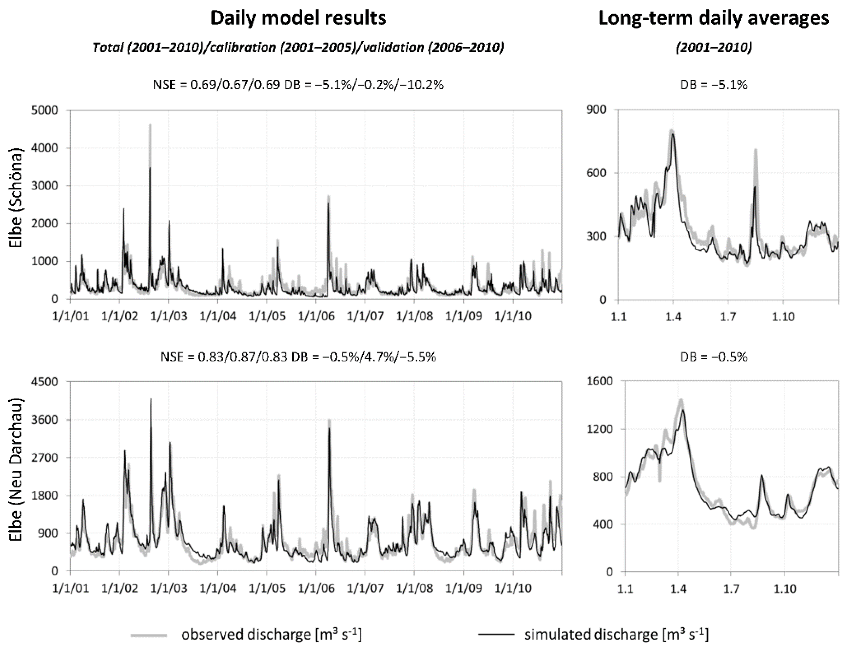
Figure 2 presents the observed and simulated daily discharges for the 10-year period (left), and the long-term daily averages (right) at the two main Elbe gauges Schöna and Neu Darchau. The discharge dynamic is well reproduced, reaching the good to very good performance ratings. The performance criteria for the daily model results are better at the downstream gauge Neu Darchau. The long-term seasonal dynamics are reproduced well at both gauges.

However, not all simulation results at the tributaries reach the same model performance (Table 6). The most difficult river to simulate was the Schwarze Elster, which is highly influenced by human activities and regulation (opencast lignite mining, discharge regulation and stream straightening), so that the hydrological processes are no longer natural. As these site-specific management measures were not implemented in the model, the model does not perform well enough at the Löben gauge. Similar problems apply to the lowland catchment of the Havel river, which is characterized by a high number of wetland areas and stream lakes, and is also highly affected by lignite mining in its upper course, all this leading to lower NSE values at gauge Havelberg.

Figure 2. Calibration results for the Elbe river discharge at the most downstream gauge Neu Darchau and the intermediate Elbe gauge Schöna (Czech/German border) for the time period 2001–2010, separated into calibration and validation sub-periods.

Table 6. Model performances for four discharge gauges of the Elbe river and six gauges of its main tributaries from the upstream to downstream location of tributaries.

**Table 6.** Model performances for four discharge gauges of the Elbe river and six gauges of its main tributaries from the upstream to downstream location of tributaries.
River	Gauge	Time Period	NSE (−)		DB (%)
River	Gauge	Time Period	Daily	Monthly	DB (%)
Elbe	Nymburk	11/2002–10/2010		0.75	−13.5
Vltava	Vranany	11/2002–10/2010		0.64	−10.5
Ohře	Louny	11/2002–10/2010		0.86	−0.3
Elbe	Schöna	2001–2010	0.69	0.77	−5.1
Schwarze Elster	Löben	2001–2008	0.25	0.60	13.4
Mulde	Bad Düben	2001–2010	0.74	0.88	1.7
Saale	Calbe-Griezehne	2001–2010	0.61	0.84	1.5
Elbe	Magdeburg	2001–2010	0.82	0.86	1.1
Havel	Havelberg	2001–2010	0.54	0.68	−1.5
Elbe	Neu Darchau	2001–2010	0.83	0.86	−0.5

Only monthly measurements for a shorter time period were available for the three gauges located in the Czech part of the Elbe basin. The best results here could be achieved for the smaller and mountainous river Ohře. The upper part of the Elbe river (gauge Nymburk), as well as the largest Elbe tributary, Vltava, show a slight underestimation of discharge. This could be explained by water regulation measures in the water course of these rivers, with a high number of barrages and dams to ensure water availability for shipping and for flood protection, which were not implemented in the model. However, the hydrological model performance in terms of NSE and DB for the Elbe and its tributaries mostly meet the aim (compare Table 3), so that it was used for the subsequent water quality calibration.

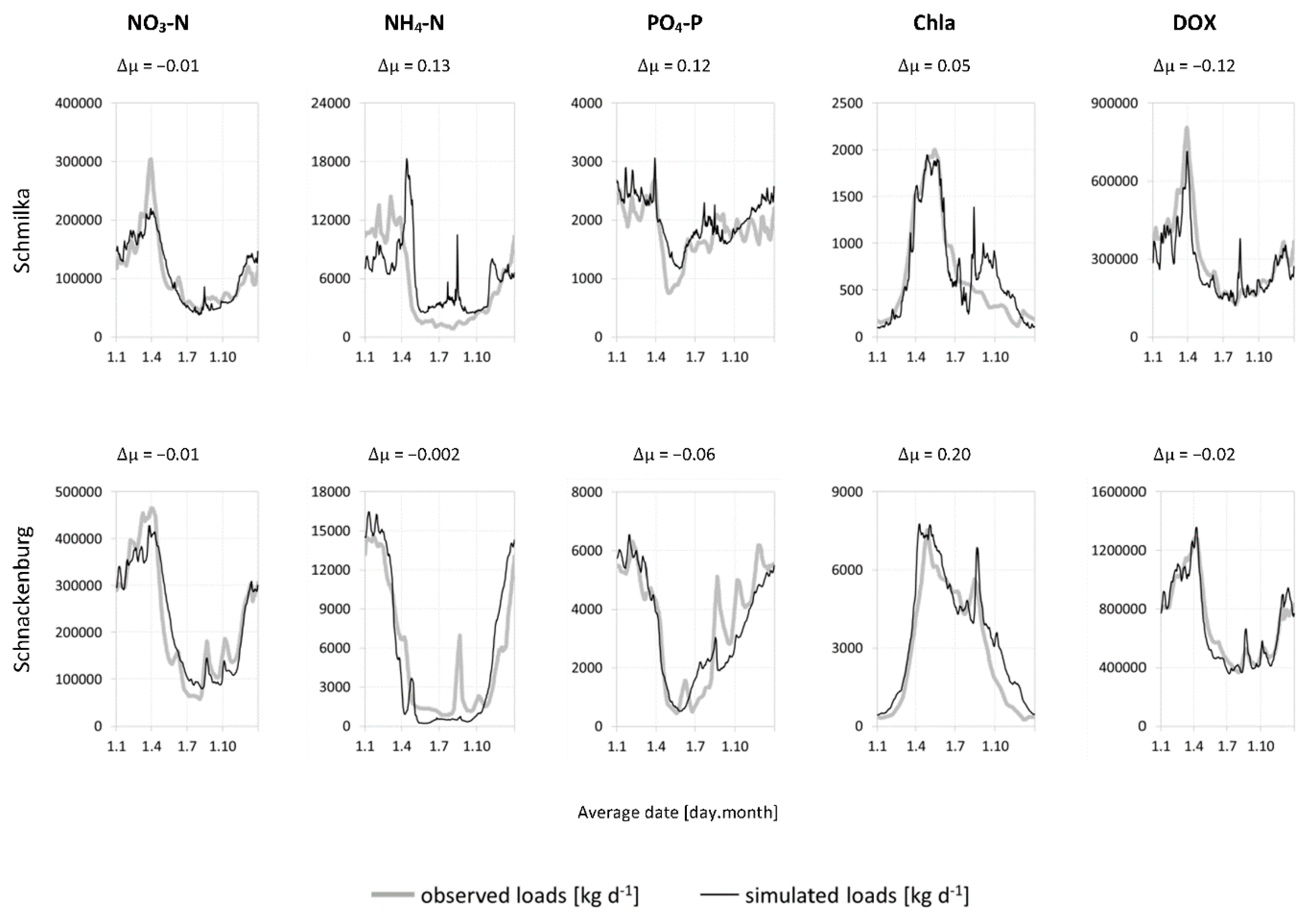
Figure 3 presents the results of water quality calibration for two main gauges in the Elbe river: Schmilka at the Czech-German border and the most downstream Elbe gauge Schnackenburg. The long-term average daily observed loads were calculated based on interpolated values between biweekly measurements and have some degree of uncertainty. The calibration was aimed at visually and statistically matching the inner-annual dynamics and minimizing the deviation in balance of the mean annual nutrient loads for the 10-year period of 2001–2010.

Figure 3. Long-term average daily observed and simulated loads of nitrate nitrogen (NO₃-N), ammonium nitrogen (NH₄-N), phosphate phosphorus (PO₄-P), chlorophyll a (Chla) and dissolved oxygen (DOX) at the two Elbe gauges Schmilka (corresponds to the total Czech loads) and Schnackenburg (most downstream gauge) for the time period 2001–2010.

In Figure 3, a specific annual cycle of the three nutrients can be observed, which is reproduced quite well by the SWIM model. The nitrate nitrogen loads (mainly coming from diffuse sources) generally follow the discharge curve with a spring peak and low values in summer. Ammonium nitrogen and phosphate phosphorus are more algae-influenced. The periods with high concentrations of chlorophyll a especially result in ammonium depletion in the river due to the high ammonium preference factor of the algae defined in the model. Algal influences on the phosphate loads are less significant, but also obvious, especially during the spring algal bloom. The dissolved oxygen loads are highly connected to the water amounts and are simulated very well. The balance measure Δμ is low in all cases and is located within the aimed range, also reflecting sufficiently good calibration results.

Figure 4 and Table 7 show results on water quality for the main tributaries of the Elbe river and for selected Elbe gauges. Figure 4 plots the simulated versus observed long-term average monthly values and illustrates the variation of the long-term seasonal cycle ratios around a diagonal of perfect fit, and Table 7 analyzes the model’s performance statistically.

Table 7. Model ability to simulate the long-term monthly average loads of water quality variables for six main tributaries as well as three selected Elbe water quality observation gauges in the time period 2001–2010 after spatially distributed model calibration. The model performance variables were calculated according to [75] and are described in Section 3.3.

**Table 7.** Model ability to simulate the long-term monthly average loads of water quality variables for six main tributaries as well as three selected Elbe water quality observation gauges in the time period 2001–2010 after spatially distributed model calibration. The model performance variables were calculated according to [75] and are described in Section 3.3.
	Vltava Zelčín	Ohře Terezín	Elbe Schmilka	Schwarze Elster Gorsdorf	Mulde Dessau	Saale Groß Rosenburg	Elbe Magdeburg	Havel Toppel	Elbe Schnackenburg
Time period	2001–2004	2007–2010	2001–2010	2004–2010	2001–2010	2001–2010	2001–2010	2001–2010	2001–2010
	NO₃-N
Δμ	−0.01	−0.09	−0.01	−0.13	0.04	0.10	0.09	−0.01	−0.01
Δσ	−0.11	−0.23	−0.04	−0.27	−0.20	0.18	0.03	−0.42	−0.07
r	0.91	0.93	0.93	0.96	0.93	0.94	0.93	0.97	0.95
	NH₄-N
Δμ	0.02	0.12	0.13	0.17	−0.08	−0.01	0.17	0.05	0.01
Δσ	0.17	−0.25	−0.23	0.02	−0.31	−0.19	0.08	0.13	0.26
r	0.64	0.74	0.68	0.53	0.85	0.97	0.92	0.94	0.95
	PO₄-P
Δμ	−0.01	0.11	0.12	0.12 *	0.03	−0.11	0.10	−0.10	−0.06
Δσ	−0.40	0.01	−0.02	0.39 *	−0.37	−0.03	0.00	−0.19	−0.03
r	0.73	0.70	0.87	0.13 *	0.87	0.93	0.92	0.24	0.94
	Chla
Δμ	0.08	−0.02	0.05	0.03	−0.08	0.04	0.06	0.12	0.20
Δσ	0.06	0.12	−0.07	0.05	0.17	0.04	−0.07	0.18	0.00
r	0.95	0.82	0.94	0.82	0.80	0.82	0.91	0.78	0.97
	DOX
Δμ	−0.06	−0.12	−0.12	0.02	−0.01	0.06	0.04	0.03	−0.02
Δσ	−0.28	−0.39	−0.30	−0.50	−0.37	0.08	−0.02	−0.25	0.02
r	0.85	0.95	0.98	0.91	0.95	0.97	0.96	0.98	0.98

Note: * 2008–2010.

Figure 4. The long-term average monthly observed and simulated discharge and loads per tributary and at two selected Elbe gauges in the period 2001–2010 (diagonals: black—perfect fit, grey—± 50% intervals).

As already detected in the hydrological calibration, the largest discrepancies between the observed and simulated values can be seen for the Schwarze Elster river. The intensive human activities within this catchment (e.g., surface water management due to lignite mining) influence nutrient processes but are not fully implemented in the model, resulting in model outputs different from observations. Some problems can also be seen for the Havel and (partly) the Mulde tributaries. The largest dispersion around the diagonal of perfect fit is obvious for ammonium nitrogen, which is difficult to model as it is highly influenced by point source emissions involving input data uncertainty as well as by algal consumption processes (parameter uncertainty). The latter, due to their complex behavior influenced by many physical, chemical and biological interactions, are difficult to model, especially in large basins. The results in terms of statistical criteria (Table 7) with mostly high r and low Δμ and Δσ confirm the visual impression.

Generally, the calibrated SWIM model for the large-scale Elbe river basin matches observations well, and can be used for climate and land use change impact assessment.

4.2. Climate Change Signals of the ENSEMBLES Scenarios

Before applying the 19 ENSEMBLES climate scenarios to the Elbe basin, they were analyzed for their trends in temperature, precipitation and solar radiation averaged over the whole basin by comparing two future scenario periods, p1 and p2, with the reference period p0. The comparison was done for the long-term average annual values as well as for the long-term average monthly values of all scenarios and periods.

The climate change signals per scenario can be found in Table 8. The results show an increase in temperature by 1.3 °C for the first period and by 3 °C for the second period on average, as well as an increase in precipitation by +41/+57 mm on average for all 19 climate scenarios. The increase in precipitation is accompanied by a decrease in solar radiation of −15/−27 J cm⁻² on average, probably due to increased cloudiness with higher precipitation amounts. There is a wide spread in signals between the scenarios, which is increasing in the second period. Regarding temperature, all scenarios agree on increasing trend, but the increase in period p2 ranges between 2 and 5 °C depending on the scenario. The agreement of the single scenarios with the overall trends is lower for precipitation (15 of 19 scenarios agree with the trend) and solar radiation (14 scenarios agree). However, a majority of scenarios correspond to the average trends.

Table 8. Climate change signals for temperature, precipitation and radiation of 19 analyzed ENSEMBLES climate scenarios and on average for the two future periods 2021–2050 (p1) and 2071–2098 (p2) compared to the reference period 1971–2000 (p0) for the Elbe basin.

**Table 8.** Climate change signals for temperature, precipitation and radiation of 19 analyzed ENSEMBLES climate scenarios and on average for the two future periods 2021–2050 (p1) and 2071–2098 (p2) compared to the reference period 1971–2000 (p0) for the Elbe basin.
Scenario	Temperature (°C)		Precipitation (mm)		Radiation (J·cm⁻²)
Scenario	p1-p0	p2-p0	p1-p0	p2-p0	p1-p0	p2-p0
S1	1.5	2.9	67	95	−26	−76
S2	2.1	4.0	−2	16	27	28
S3	1.7	3.4	34	17	8	7
S4	2.2	5.0	48	−49	1	43
S5	1.8	4.1	104	94	−57	−67
S6	1.7	3.5	24	13	−22	−12
S7	0.9	2.6	35	110	−12	−20
S8	0.7	1.9	63	86	−30	−48
S9	0.8	2.4	47	112	−29	−65
S10	0.9	2.6	14	47	−18	−42
S11	1.1	2.8	−4	−68	5	36
S12	0.9	2.0	14	−31	−16	−111
S13	0.6	2.0	57	157	−21	−73
S14	0.9	2.5	37	99	−29	−47
S15	0.9	2.6	29	87	1	7
S16	1.0	3.1	52	63	−12	−5
S17	1.4	3.3	65	54	−22	−11
S18	0.9	2.6	36	99	−16	−20
S19	1.8	3.9	50	76	−26	−40
mean_all	1.3	3.0	41	57	−15	−27
stdev_all	0.5	0.8	26	60	18	42

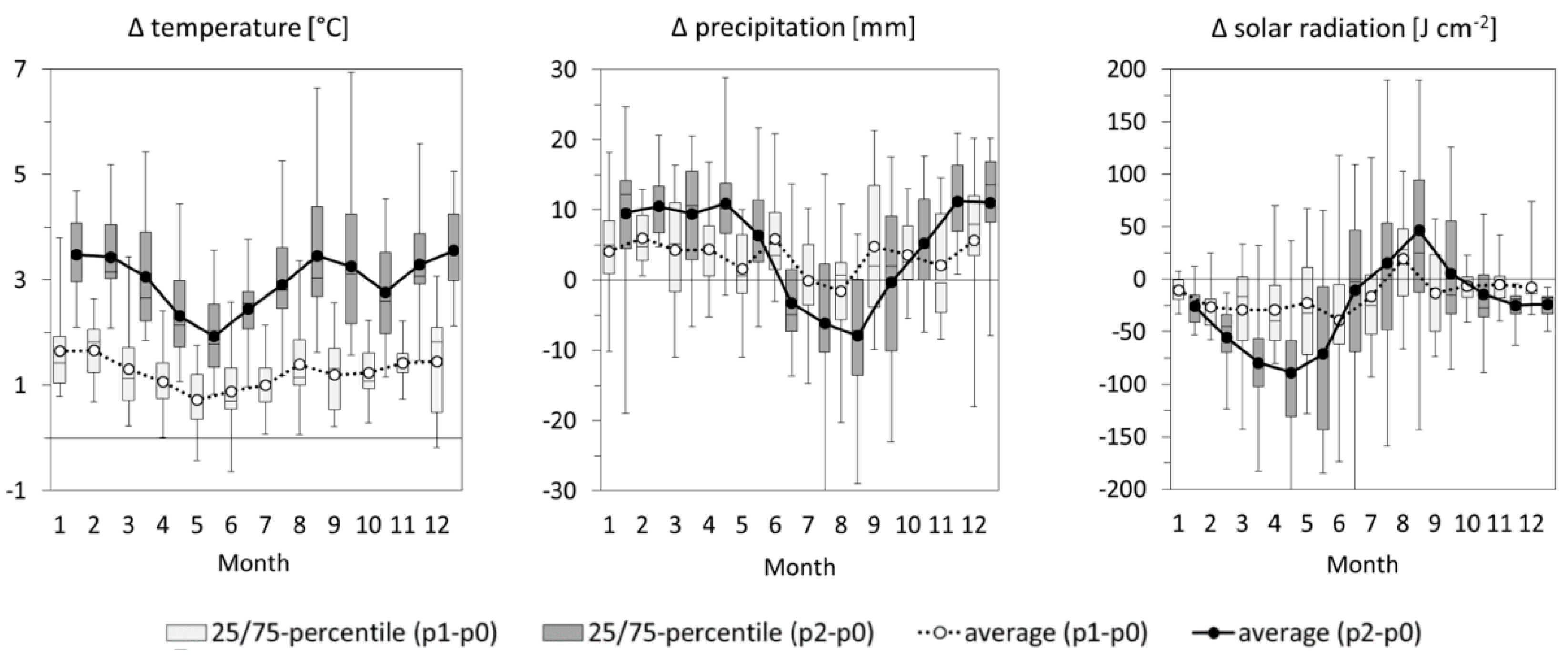
The seasonal climate change signals are visualized in Figure 5. Looking at the changes per month, it is obvious that the value as well as the spread of the climate change signals is higher in the second period. The increase in temperature is confirmed for the entire course of the year, and it is lowest in May and highest in winter months (December–February) and in August. The changes in precipitation and solar radiation vary around the zero-line and show an opposite behavior (probably due to connection of precipitation and cloudiness). In the first period precipitation is slightly decreasing in July and August, and in the second period negative changes in precipitation are projected from June to September. The changes in solar radiation show almost the opposite trends. In general, the 19 ENSEMBLES climate scenarios project a warmer and wetter climate with less sunshine hours from autumn to spring, but a warmer, dryer and sunnier climate in the summer months for the region.

Figure 5. Ranges of seasonal climate change signals for temperature, precipitation and solar radiation of 19 ENSEMBLES climate scenarios for the two future periods compared to the reference period of the same scenario for the Elbe basin. The plots represent median (line), 25th/75th percentiles (box), min/max values (whiskers) and the average (dots) change of all 19 scenarios.

4.3. Climate Change Impacts

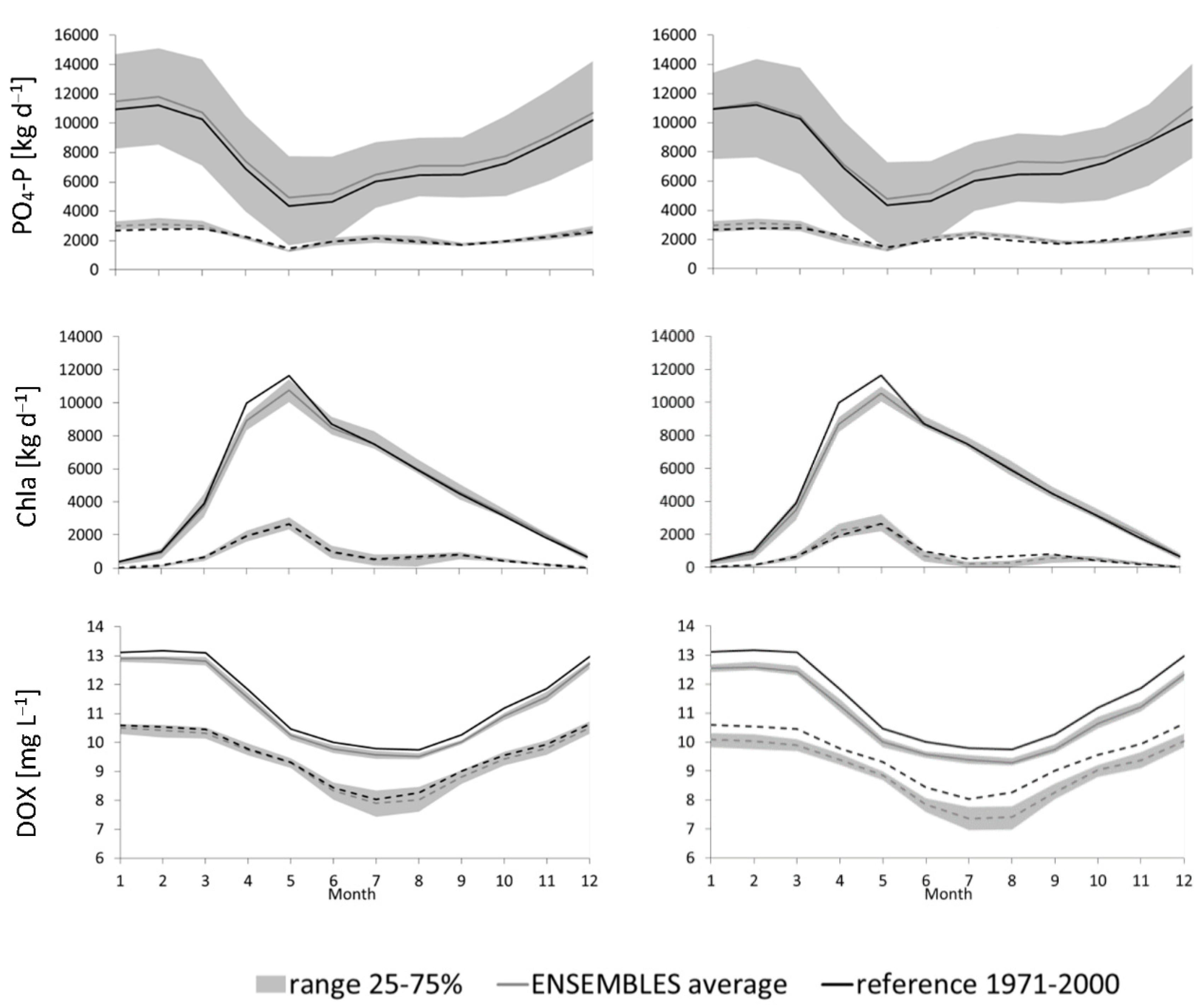
The projected changes in climate lead to changes in simulated water quantity and quality variables in the Elbe basin in future periods. The results are shown Figure 6 for the two Elbe river gauges Schöna and Neu Darchau. They present changes in the long-term average seasonal dynamics comparing the average and the 25th/75th percentile ranges of six variables from simulations driven by 19 climate scenarios in the future and the average of the reference period 1971–2000.

Figure 6. The long-term average monthly values of simulated discharge (Q), nutrient and chlorophyll a loads (NO₃-N, NH₄-N, PO₄-P, Chla) and dissolved oxygen concentrations (DOX) with uncertainty ranges (25th/75th percentiles corresponding to 19 simulations) at the two Elbe gauges Neu Darchau (full lines) and Schöna (dashed lines) for the future periods 2021–2050 (p1, a) and 2071–2078 (p2, b) in comparison to the corresponding average values of the reference period 1971–2000 (p0).

Following the increasing trend for precipitation in the Elbe basin, the discharge is projected to increase as well, both at the last Elbe gauge and at the gauge of the Czech-German border. The increase can be observed during almost the whole year, with the highest values in winter months (due to higher rainfall) and the lowest values, or even negative changes in the p1 period, in April (due to lower or missing snow melt peaks). Though a decrease in precipitation is projected in the summertime (compare Figure 5), the projected discharge in summer months is higher than in the reference period, probably due to the capability of soils to retain additional winter and spring water causing delayed subsurface and groundwater flows. However, the uncertainty ranges for the projected discharge are quite high, especially at the most downstream gauge.

The nitrate nitrogen load performs similarly to the discharge, as nitrate nitrogen comes to the river mainly dissolved in water from diffuse sources. A moderate increase can be observed in the first winter months, followed by some decrease in spring, whereas the second half of the season shows only minor changes on average compared to the reference period (due to higher retention time of nitrate nitrogen compared to water as well as impacts of vegetation).

The ammonium nitrogen loads are higher on average in the upstream part of the Elbe (gauge Schöna) than downstream (gauge Neu Darchau) due to higher loads in the Czech part of the catchment as well as to progressively increasing phytoplankton concentration downstream of the Elbe. The decrease in ammonium load caused by changes in climate conditions is obvious in the first half of the season (especially during spring flood). The decrease in NH₄-N loads is probably connected to the rising temperatures, as mineralization processes and the emergence of leachable ammonium in soils are temperature-related and occur mainly within a certain temperature range. The uncertainty ranges around the ENSEMBLES average, representing the most probable 50% of the 19 scenario results, are quite narrow.

The average phosphate phosphorus load shows a slight and almost constant increasing trend throughout the season, but the uncertainty ranges are the largest for this nutrient, caused by the high uncertainty and climate-dependence of phosphorus-related processes in the Havel catchment (compare with Figure 7). The increase in loads is probably connected to increasing erosion and leaching processes with higher precipitation in the future, washing more phosphorus from sandy and highly permeable soils. It could also be a result of less ingestion by a decreasing algae population in the future.

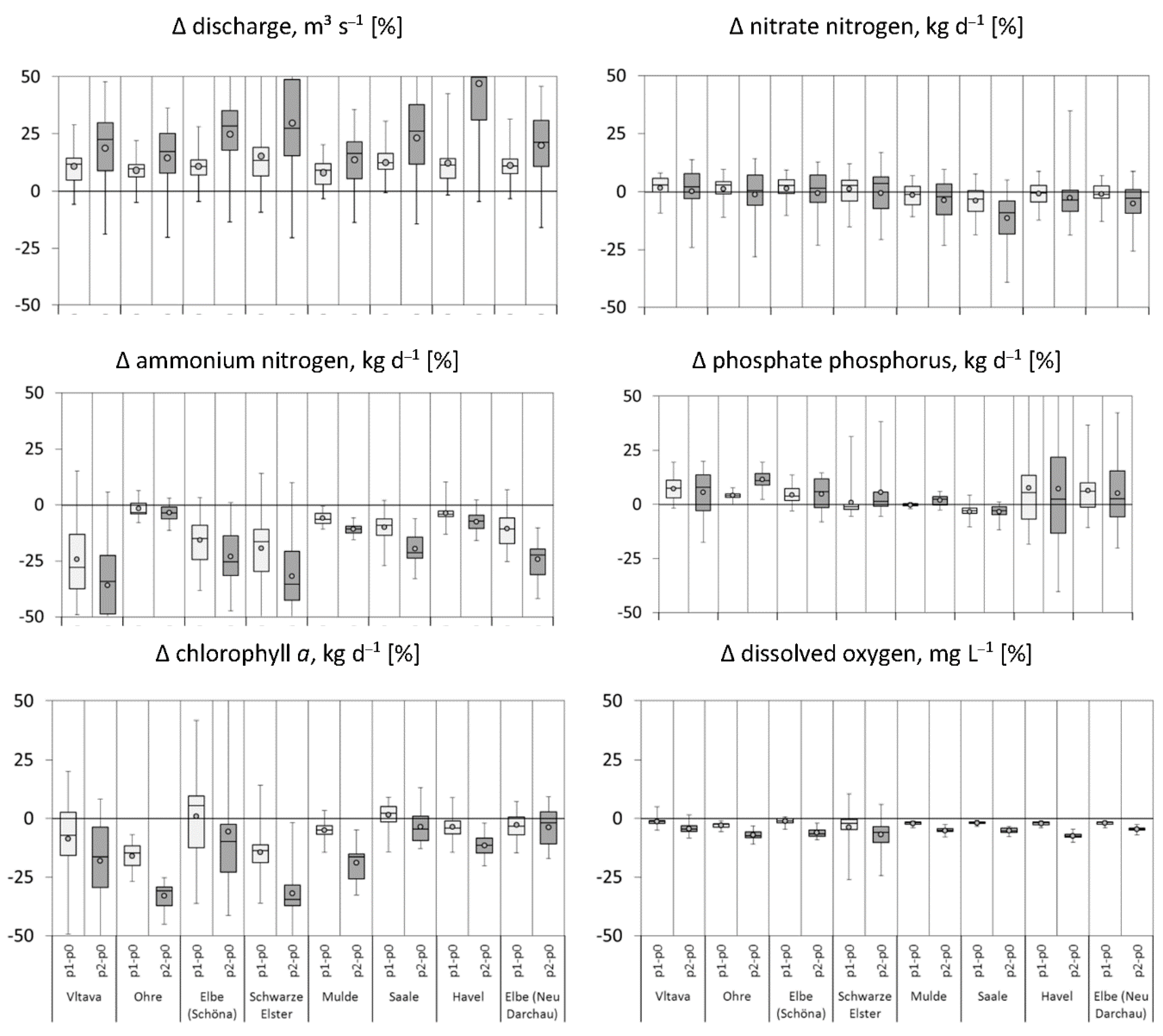
Figure 7. Ranges of the percental changes of 30-year-average river discharges, nutrients and chlorophyll a loads, as well as dissolved oxygen concentrations in the Elbe river and its main tributaries simulated with SWIM driven by 19 ENSEMBLES climate scenarios (in future periods p1 (light) and p2 (dark) compared to the reference period p0 of the same scenario). The plots visualize the following ranges: min/max (whiskers), 25th/75th percentiles (boxes), median (line) and average (dots) changes of all 19 scenarios.

The chlorophyll a load is projected to decrease in the spring blossom time, when warmer temperatures (temperature stress) and lower solar radiation (below the optimum value) may hamper phytoplankton growth and less ammonium is available for algae consumption.

The dissolved oxygen concentration in the Elbe river is projected to decrease, and the changes remain almost constant throughout the season. This is probably connected to the increasing water temperature, resulting in lower values of oxygen saturation in the water. The uncertainty ranges for future dissolved oxygen concentrations are higher upstream, probably due to the generally higher ammonium loads modeled in the upper river reaches, where oxygen is used for nitrification in the water column.

In addition to the temporal analysis of climate impacts, Figure 7 illustrates some spatially distributed results for the Elbe and its tributaries. For that, average percental changes were calculated for six main tributaries of the Elbe and two Elbe gauges (the same as in Figure 6).

The overall trend for the entire basin can be generally detected regarding different variables in Figure 7, though there are some outlying sub-catchments. For all gauges an increasing discharge is projected, which becomes higher in the second period. Also, the uncertainty ranges increase in p2. The differences between gauges are small.

The nitrate nitrogen load decreases on average for the entire Elbe river basin (Neu Darchau). The decrease is largest for the Saale catchment, which is characterized by the highest share of agricultural areas due to very fertile soils with a high nutrient retention capability. There are also some sub-catchments where a small increase (or no change) in nitrate load on average is simulated. This is probably connected to an increased diffuse pollution with increased precipitation in these sub-areas.

The impacts on ammonium nitrogen loads are almost all negative, and show a high diversity between the sub-catchments. The uncertainty ranges are highest in the Vltava and Schwarze Elster sub-catchments, where ammonium pollution is generally at its highest level, and have more space for variability due to climate change impacts.

Except for the Saale sub-catchment with its fertile soils and high nutrient retention potential, the climate change impact on phosphate phosphorus shows increasing loads due to increased leaching and erosion processes. The uncertainty ranges are extremely high in the Havel sub-catchment, where phosphorus contamination is the highest in the Elbe drainage area, and a high share of permeable and sandy soils causes a high phosphorus leaching potential with higher precipitation amounts.

Chlorophyll a demonstrates a decreasing trend on average almost everywhere. The uncertainty ranges, especially in the upper tributaries, are quite high, due to the high complexity of algae processes simulated in the model, which are influenced by many system-internal and external drivers.

Changes in the dissolved oxygen concentrations have a very small uncertainty range and show a decreasing trend on average for all gauges due to increased temperatures and lower oxygen saturation capacity. The highest range in average changes can be observed for the Schwarze Elster sub-catchment, which is quite heavily polluted with ammonium nitrogen. The latter is highly sensitive to climate change impacts and is connected to the oxygen processes in the river water.

4.4. Socio-Economic Change Impacts under Climate Change

In addition to the climate change impact assessment, five land use change experiments were run to test the model’s reaction on certain management measures aimed at reducing nutrient inputs to the river network. The aim was to check whether such measures are able to be reversed, intensify or revoke climate change impacts. The land use change experiments were run 19 times, driven by the 19 ENSEMBLES climate scenarios for the near future period 2021–2050 (p1), and the results were compared with the results achieved under the reference management conditions for the period 1971–2000 (p0) of the same scenarios (combined impacts) as well as with the climate scenario-driven results with the reference management for period p1 (land use change impacts only).

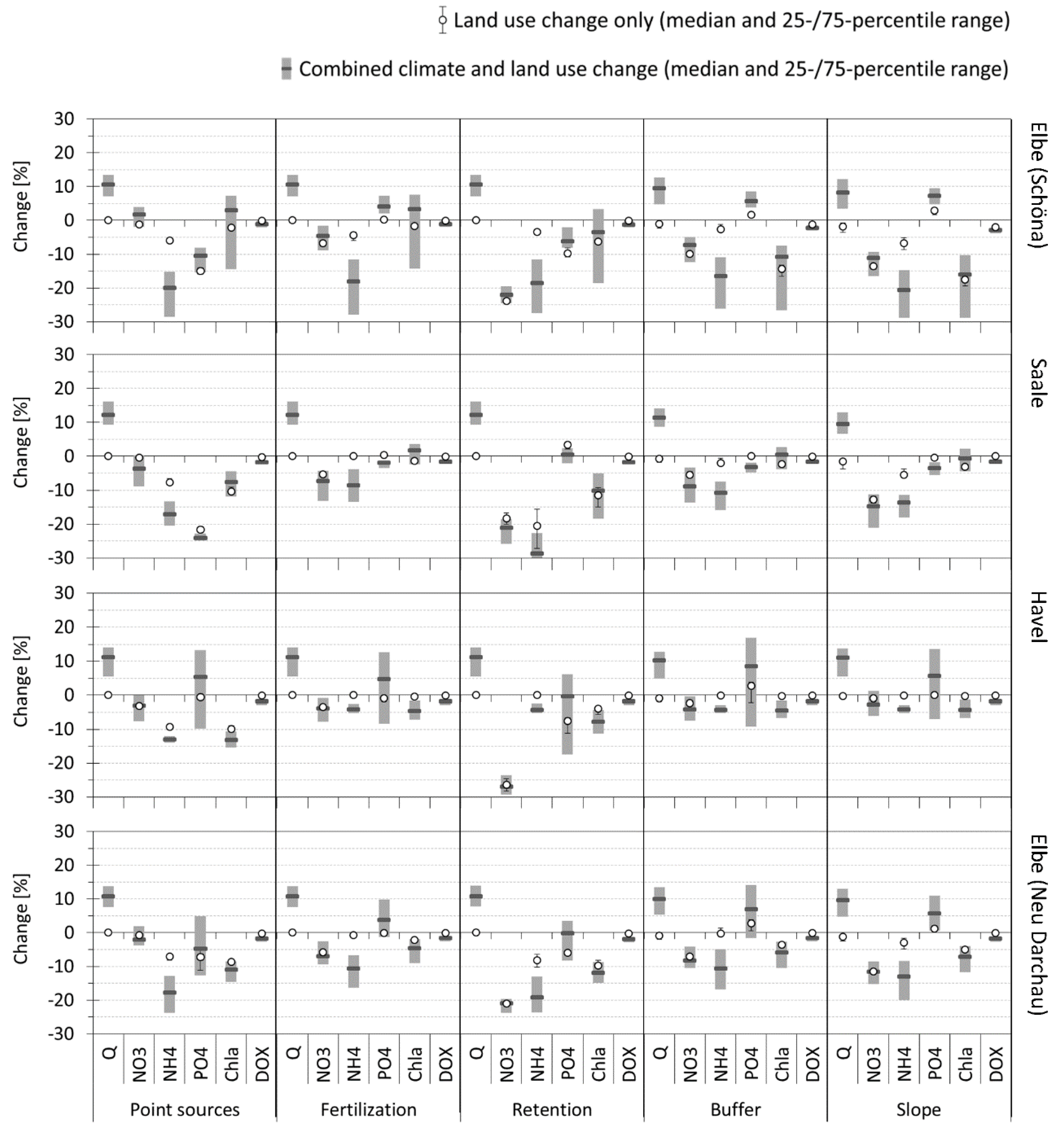
The single and combined impacts were analyzed for the two Elbe gauges Schöna (Czech/German border) and Neu Darchau (Elbe outlet) as well as for the outlets of the two selected tributaries Saale and Havel (Figure 8). The results are shown as median values with a 25th/75th percentile range. In some cases, even the single land use change impact shows some range of relative changes caused by different behavior of temperature- and water-dependent nutrient processes under different climate conditions used as an external driver.

Figure 8. Impacts of socio-economic changes and combined climate and socio-economic changes on the average water discharge (Q), nutrient (NO₃-N, NH₄-N, PO₄-P) and chlorophyll a (Chla) loads and dissolved oxygen concentrations (DOX) of the Elbe river at two stations and at two main German tributaries. The dark grey bars and white dots show the median of 19 percental changes together with their 25th/75th percentile ranges (light grey ranges and black whiskers).

The socio-economic changes related to nutrient inputs to the river network (experiments “Point sources” and “Fertilization”) and an increased nutrient retention potential in soils (experiment “Retention”) have no influence on water discharge. Only the combined impacts show an increase in discharge of about 10% due to climate change. The solely socio-economic impacts of a changed land use composition (“Buffer” and “Slope”) on river discharge show a decrease (due to increased evapotranspiration of the enlarged grassland areas), but it is quite low, and cannot compensate the increase in Q caused by the projected climate change, so that all combined impacts for these experiments have a positive direction.

The reduction of point source emissions has the highest influence on phosphate and ammonium loads, as these nutrients mainly originate from anthropogenic inputs of water treatment plants or industrial units. The projected climate change even intensifies the reduction of ammonium nitrogen loads in the rivers, whereas the decrease of phosphate phosphorus is reduced by climate change impacts (except for the Saale basin). The sole reduction of point source emissions predominantly results in a decrease of chlorophyll a loads in the rivers due to less available ammonium and phosphate as algal food.

The decrease in fertilizer application causes lower nitrate loads in all analyzed river parts, as this nutrient originates mainly from diffuse sources (predominantly from agricultural fields). The reduction is only marginally influenced by climate change. A decrease in fertilization affects NH₄-N only partly, and causes decreased ammonium loads, particularly in the upper part of the Elbe basin. As the changes in NH₄-N and PO₄-P loads are less distinct under the “Fertilization” experiment, chlorophyll a loads are only marginally influenced. The on-average-increasing chlorophyll a trend caused by climate change impacts in the upper Elbe and Saale catchments cannot be reversed by a simple reduction of fertilization in the combined experiments.

An increased nutrient retention and decomposition potential in the soils of the landscape (“Retention”) has the highest impact on nutrient loads. Especially the diffuse nitrate nitrogen loads are affected, but also ammonium and phosphate show some reactions, though with different magnitudes for the four analyzed gauges. The diversity in the magnitude of changes for the river parts can be explained by the heterogeneity and distribution of land use patterns and point sources as well as by the diversity in projected climate change within the catchment. As NH₄-N and/or PO₄-P are remarkably reduced under the retention experiment, chlorophyll a shows a decreasing trend due to a lack of nutrients. This reduction is even able to reverse the increasing trend in chlorophyll a caused by climate changes in the upper Elbe and Saale sub-catchments.

Two experiments dealing with a changed land use composition (“Buffer” and “Slope”) result in more meadows and less agricultural areas in the sub-catchments and show similar results in the different river parts. Nitrate nitrogen is reduced most in the majority of cases due to less agricultural area with fertilizer application and hence lower total fertilizer loading under the experiments. The highest diversity of changes can be seen under the “Slope” experiment in the upper Elbe and Saale sub-catchments, which are characterized by a high share of mountainous areas, where the share of transformed land use areas is higher than in the lowland sub-catchment of the Havel river. For the latter, the “Slope” experiment has nearly no impact on the model outputs, and the combined changes result only from the climate scenario impacts.

The concentrations of dissolved oxygen are not visibly influenced by the changes in land use or management. The decreasing trend due to increased water temperature is more obvious in the upper part of the Elbe basin (gauge Schöna), probably due to less oxygen production with decreasing chlorophyll a loads in the river.

In general, the shares of cropland and distribution of point sources, as well as the distribution of soils with their specific nutrient retention potentials, are very important factors influencing the nutrient loads coming with the rivers. However, in the model application presented here, it is often difficult to distinguish between the single impacts on nutrient loads caused by certain land use or management changes and the secondary impacts due to altered chlorophyll a concentrations and a resulting change in nutrient uptake in the water body. The in-stream processes include a complex behavior of nutrients with a high number of interactions and feedbacks with the algae population. Chlorophyll a, for example, increases with decreasing NH₄-N availability and vice versa, causing increase (or decrease) of PO₄-P due to less (or more) algal uptake. Therefore, the resulting impacts are not only directly caused by land use changes, but are also indirectly caused by the subsequently changed conditions in the river water.

5. Discussion

A comparison of obtained results with the results of previous studies dealing with global change impacts in the Elbe river catchment is sometimes difficult, as different scenarios and downscaling methods were used by different authors. The whole range of model outputs illustrates a high uncertainty in climate change impact assessment.

The majority of published studies for the Elbe basin deal with climate change impacts on the hydrological cycle. The simulated effects of climate change on water cycle and river discharge presented in literature are diverse and differ in intensity and even in direction of change, resulting mainly from the diversity of precipitation change signals projected by different climate scenarios. Studies using 100 realizations of the Statistical Analogue Resampling Scheme (STARS), with a distinct decrease in summer precipitation and a moderate increase of precipitation in winter, project lower river discharge in the Elbe basin [85,86,87,88]. However, we have to note that recently the STARS model was critically discussed [89,90] regarding its suitability for producing climate scenarios. Model runs using the Inter-Sectoral Impact Model Intercomparison Project (ISI-MIP) climate scenarios [91] for the Elbe basin also project a decreased discharge on average, but the magnitude of changes is less pronounced [85]. Huang et al. [92] report diverse results depending on the driving climate model: the projections driven by the empirical-statistical model WETTREG (WETTerlagen-basierte REGionalisierungsmethode) produce negative trends in flood occurrence, whereas the projections forced by the two dynamical regional climate models REMO (REgional MOdelling) and CCLM (COSMO-Climate Limited-area Modelling) show various results with the prevalence of increasing trends in flood occurrence for this region. Applications of the ENSEMBLES scenarios for assessing future risks of floods and droughts in Germany showed an increasing trend of floods but no significant increase in droughts for the Elbe basin [22]. This is also reflected in our study, where under the same ENSEMBLES climate scenarios’ higher discharges are projected on average (compare Figure 7).

There are some studies on the management change impacts on river water quality for often only small parts of the Elbe region (e.g., [93,94,95]), but only a few publications exist covering water quality issues under climate change. So, Quiel et al. [62] used the outputs of a model chain driven by selected realizations of the statistical model STARS as boundary conditions to run the river model QSim for a 700 km reach of the Elbe river. Soluble phosphorus concentrations decrease in all tributaries under all scenarios compared with the reference period for the same scenario. This results in an increased phytoplankton growth along the studied river reach and a shift of the chlorophyll a maximum under the dry and medium scenarios, but in a decrease in chlorophyll a concentration under the wet scenario conditions [62]. The latter is in accordance with the results for chlorophyll a presented in our study (compare Figure 7), as the ENSEMBLES climate projections produce a wetter climate in the future as well.

It seems that the projected nutrient loads presented in literature often correspond to the precipitation change signals, especially when eco-hydrological models using a simple routing of nutrients through the river network are applied. The increased precipitation causes higher nitrogen leaching through soils as well as higher phosphorus erosion rates with surface flow to the river network. Both processes increase nutrient loading to the river waters. Therefore, statistically downscaled climate scenarios with a negative trend in precipitation (e.g., STARS) mostly project decreasing nutrient loads in the Elbe catchment, whereas dynamic climate scenarios (e.g., REMO or the wet years of ISI-MIP scenarios) mostly result in increasing nutrient loads in the river due to positive precipitation change signals (e.g., [96,97]). This simple relationship between precipitation change signals and final nutrient load projections can be disturbed by including in-stream and algal processes in the eco-hydrological models, due to included transformation and ingestion of nutrients in the river network.

Nevertheless, the same conclusion as for river discharge is valid for the water quality impact assessment: a wide range in projections can be found in literature (as well as in our study). However, the diversity in discharge and water quality projections may not necessarily be the result of the application of different model approaches or climate scenario sets. Even with one scenario and one model, a high spatial variability can be observed, and some sub-regional trends can actually be opposite to the overall average trend of a large-scale basin, or local effects can be masked by large-scale aggregation [78,79]. This could also be seen in our study, where changes of model outputs due to climate impact differ in magnitude and intensity or even in the direction of change when comparing several tributaries of the Elbe (Figure 7).

In climate and socio-economic impact assessments in addition to the general (and often large) uncertainty associated with climate scenarios as drivers, there is also uncertainty connected to applied watershed models. The so-called structural and parameterization uncertainty is related to the ability of eco-hydrological models to represent the interrelated processes in landscape, vegetation and river network. The parameterization uncertainty can be especially large in a model with a high number of calibration parameters influencing each other, as in the SWIM model with implemented in-stream processes. Often several calibration parameter combinations exist, delivering the same or very similar model performance, so that it could happen to be “right for the wrong reasons” [98,99]. In general, such uncertainty rises with the rising model complexity, and goes along with a rising need in calibration efforts [68], and this should be taken into account when the model is extended by adding new processes. To overcome the limitations and weaknesses of a single eco-hydrological or climate model approach, it is useful to apply several models with the same input parameter sets (model intercomparison) and ensembles of climate scenarios for a more comprehensive assessment of uncertainties and elicitation of robust outputs [91,100].

The land use change experiments applied in this study do not represent the “full” set of potential future land use scenarios in the Elbe region, which could be elaborated considering options of future socio-economic development. For example, changes in urbanization or forest patterns could also have effects on the environment and the water resources [101,102]. In our study only the effects of single measures connected to nutrient sources and agricultural practices (which are currently considered in the planning of land/water management) on water quantity and quality were tested, also in combination with climate change. This could be regarded as a first step to finding suitable methods for adaptation to climate change impacts. However, for further studies it is recommended to apply a combination of different measures under consideration of the future socio-economic development for a more realistic land use change impact assessment. As climate change can strengthen, revoke or even inverse the land use change impacts, this aspect should always be included in such studies.

6. Summary and Conclusions

The SWIM model supplemented by an in-stream module was successfully calibrated and validated for the entire Elbe river basin, and applied for climate and land use change impact assessment in the region. For that, the commonly used technique was applied, using 19 climate scenario data sets provided by the ENSEMBLES project to drive an eco-hydrological model for 30-year periods in order to evaluate changes in water quantity and quality for the two future periods of 2021–2050 and 2071–2098 in comparison to the reference period of 1971–2000.

The calibration and validation of the extended SWIM for the Elbe region was complicated due to the high number of calibration parameters and the spatial variability within the catchment. Satisfactory model results could be still achieved by applying spatially distributed calibration parameter sets to capture variability in soil type distribution, land use pattern and economic development in the sub-catchments.

The analysis of a potential future climate, as projected by 19 scenarios for the Elbe catchment, indicates increasing trends in temperature and precipitation, but a decreasing trend in solar radiation on average. However, looking at the climate change signals of the 19 scenarios separately, differences can be seen in the intensity and—for precipitation and solar radiation—also in the direction of change signals. The standard deviation of the whole set of climate change signals increases in the second future period.

The results of the climate change impact assessment on water quantity and quality show a high spatial variability within the catchment according to the individual characteristics of the tributaries within the basin. For the entire Elbe catchment, river discharge is projected to increase by 11% and 20% on average for the two future periods. Dissolved oxygen concentration is projected to decrease by 2% and 5%, mainly due to the increased water temperature. The projected changes in nutrient loads do not show the same change direction. While NO₃-N loads slightly decrease on average (−1% and −5%), and NH₄-N shows a distinct decreasing trend (−11% and −24%), PO₄-P loads are expected to increase by 6% and 5% on average. The simulated reaction of nutrient loads to climate change is always influenced by the phytoplankton population, and vice versa. The chlorophyll a concentrations decrease slightly under the future conditions, by 3% and 4% on average, at the last downstream Elbe gauge.

Five simulation experiments dealing with possible changes in nutrient emissions were applied in the study, also in combination with climate change scenarios. Water discharge was mainly influenced by climate change impacts, and land use change measures had little or no influence on runoff. A reduction of agricultural area or fertilizer application mainly influenced the resulting nitrate nitrogen loads in the Elbe, whereas the reduction of point source emissions had the highest impacts on ammonium nitrogen and phosphate phosphorus loads. The chlorophyll a concentrations reacted to a changed food supply in the river, and would be reduced with a reduced nitrogen and phosphorus availability. An increase in nutrient retention and decomposition potential within the catchments would certainly be beneficial to reduce all types of nutrient loads in the river waters.

Nevertheless, the model application in the Elbe basin comes along with a certain degree of structural, parameterization and scenario uncertainty. Due to the lack of more detailed information on the case-specific observations and processes, not all possible methods to reduce uncertainties could be applied in this study, and the climate scenario–related uncertainty is unavoidable. The climate change impact assessment and land use change simulation experiments presented here deliver the first results and rough estimation on probable future developments in the Elbe river basin under climate change. For future research, in order to diminish and better assess (but not to eliminate) uncertainty, it could be recommended to apply two to three eco-hydrological models, as well as a “full” set of socio-economic scenarios, for a more reliable combined climate and land use change impact assessment. It could be also advantageous to additionally include management measures neglected in this model application so far (e.g., reservoirs or different crop types and rotations). These methods would help to identify future risks and threats more realistically, and to virtually test possible adaptation measures, as efforts to cope with the future climate conditions and their impacts are generally needed. Watershed models offer a suitable tool to guide decision-making on water quantity and quality for a sustainable management of water resources to match the requirements of the European Water Framework Directive (WFD).

Acknowledgments

The ENSEMBLES data used in the study were produced in the EU FP6 Integrated Project ENSEMBLES (contract No. 505539). The authors thank Shaochun Huang for delivering the prepared spatial SWIM input data of the entire Elbe river basin. The authors additionally thank Vanessa Wörner for download and preparation of observed water quality data, and Lasse Scheele for climate scenario data download, preparation and evaluation.

Author Contributions

The two authors planned and designed the methods to study climate and management change impacts on water quantity and quality in the Elbe river catchment. Cornelia Hesse set up, adjusted and calibrated the extended SWIM model with included in-stream processes for the Elbe river catchment, ran the climate and land use change scenarios and analyzed the temporal and spatial scenario output data. Cornelia Hesse also prepared the tables and figures for the publication, wrote the text and formatted the paper. Valentina Krysanova guided and supervised the whole process, discussed results during the modeling study, and edited the manuscript.

Conflicts of Interest

The authors declare no conflict of interest.

References

Intergovernmental Panel on Climate Change (IPCC). Climate Change 2007: The Physical Change Basis. Contribution of Working Group I to the Fourth Assessment Report of the Intergovernmental Panel on Climate Change; Solomon, S., Qin, D., Manning, M., Chen, Z., Marquis, M., Averyt, K.B., Tignor, M., Miller, H.L., Eds.; Cambridge University Press: Cambridge, UK; New York, NY, USA, 2007; p. 996. [Google Scholar]
Intergovernmental Panel on Climate Change (IPCC). Summary for Policymakers. In Climate Change 2013: The Physical Science Basis. Contribution of Working Group I to the Fifth Assessment Report of the Intergovernmental Panel on Climate Change; Stocker, T.F., Qin, D., Plattner, G.-K., Tignor, M., Allen, S.K., Boschung, J., Nauels, A., Xia, Y., Bex, V., Midgley, P.M., Eds.; Cambridge University Press: Cambridge, UK, 2013; pp. 3–29. [Google Scholar]
European Environment Agency (EEA). The European Environment. State and Outlook 2010. Land Use; EEA: Copenhagen, Denmark, 2010. [Google Scholar]
Cassardo, C.; Jones, J.A.A. Managing water in a Changing World. Water 2011, 3, 618–628. [Google Scholar] [CrossRef]
Research Institute for Knowledge Systems (RIKS). Exploration of Land Use Trends under SOER 2010; RIKS: Maastricht, The Netherlands, 2010. [Google Scholar]
Alcamo, J.; Flörke, M.; Märker, M. Future long-term changes in global water resources driven by socio-economic and climatic changes. Hydrolog. Sci. J. 2007, 52, 247–275. [Google Scholar] [CrossRef]
Christensen, O.B.; Christensen, J.H. Intensification of extreme European summer precipitation in a warmer climate. Glob. Planet. Chang. 2004, 44, 107–117. [Google Scholar] [CrossRef]
Kløve, B.; Ala-Aho, P.; Bertrand, G.; Gurdak, J.J.; Kupfersberger, H.; Kværner, J.; Muotka, T.; Mykrä, H.; Preda, E.; Rossi, P.; et al. Climate change impacts on groundwater and dependent ecosystems. J. Hydrol. 2014, 518, 250–266. [Google Scholar]
Kundzewicz, Z.W. Climate change impacts on the hydrological cycle. Ecohydrol. Hydrobiol. 2008, 8, 195–203. [Google Scholar] [CrossRef]
Wang, X.; Siegert, F.; Zhou, A.; Franke, J. Glacier and glacial lake changes and their relationship in the context of climate change, Central Tibetan Plateau 1972–2010. Glob. Planet. Chang. 2013, 111, 246–257. [Google Scholar] [CrossRef]
Linderholm, H.W. Growing season changes in the last century. Agric. For. Meteorol. 2006, 137, 1–14. [Google Scholar] [CrossRef]
Vittoz, P.; Cherix, D.; Gonseth, Y.; Lubini, V.; Maggini, R.; Zbinden, N.; Zumbach, S. Climate change impacts on biodiversity in Switzerland: A review. J. Nat. Conserv. 2013, 21, 154–162. [Google Scholar] [CrossRef]
Kittel, T.G.F. The Vulnerability of Biodiversity to Rapid Climate Change. In Climate Vulnerability: Understanding and Addressing Threats to Essential Resources; Pielke, R.A., Ed.; Elsevier Inc., Academic Press: Oxford, UK, 2013; Volumn 4, Chapter 4; pp. 185–201. [Google Scholar]
Lindner, M.; Fitzgerald, J.B.; Zimmermann, N.E.; Reyer, C.; Delzon, S.; van der Maaten, E.; Schelhaas, M.-J.; Lasch, P.; Eggers, J.; van der Maaten-Theunissen, M.; et al. Climate change and European forests: What do we know, what are the uncertainties, and what are the implications for forest management? J. Environ. Manag. 2014, 146, 69–83. [Google Scholar] [CrossRef] [PubMed]
Gabriel, K.M.A.; Endlicher, W.R. Urban and rural mortality rates during heat waves in Berlin and Brandenburg, Germany. Environ. Pollut. 2011, 159, 2044–2050. [Google Scholar] [CrossRef] [PubMed]
Haines, A.; Kovats, R.S.; Campbell-Lendrum, D.; Corvalan, C. Climate change and human health: Impacts, vulnerability and public health. Public Health 2006, 120, 585–596. [Google Scholar] [CrossRef] [PubMed]
Koch, H.; Vögele, S.; Hattermann, F.F.; Huang, S. Sensitivity of electricity generation in Germany to climate change and variability. Meteorol. Z. 2015. in print. [Google Scholar]
Liersch, S.; Cools, J.; Kone, B.; Koch, H.; Diallo, M.; Reinhardt, J.; Fournet, S.; Aich, V.; Hattermann, F.F. Vulnerability of rice production in the Inner Niger Delta to water resources management under climate variability and change. Environ. Sci. Policy 2013, 34, 18–33. [Google Scholar] [CrossRef]
Alcamo, J.; Moreno, J.M.; Nováky, B.; Bindi, M.; Corobov, R.; Devoy, R.J.N.; Giannakopoulos, C.; Martin, E.; Olesen, J.E.; Shvidenko, A. Europe. In Climate Change 2007: Impacts, Adaptation and Vulnerability; Contribution of Working Group II to the Fourth Assessment Report of the Intergovernmental Panel on Climate Change; Parry, M.L., Canziani, O.F., Palutikof, J.P., van der Linden, P.J., Hanson, C.E., Eds.; Cambridge University Press: Cambridge, UK, 2007; pp. 541–580. [Google Scholar]
European Environment Agency (EEA). Climate Change, Impacts and Vulnerability in Europe 2012; EEA-Report No 12/2012; EEA: Copenhagen, Denmark, 2012; p. 300. [Google Scholar]
Federal Environmental Agency (UBA). Monitoringbericht 2015 zur Deutschen Anpassungstrategie an den Klimawandel—Bericht der Interministeriellen Arbeitsgruppe Anpassungsstrategie der Bundesregierung; UBA: Dessau-Roßlau, Germany, 2015. [Google Scholar]
Huang, S.; Krysanova, V.; Hattermann, F.F. Projections of climate change impacts on floods and droughts in Germany using an ensemble of climate change scenarios. Reg. Environ. Chang. 2015, 15, 461–473. [Google Scholar] [CrossRef]
Kyselý, J.; Beranová, R. Climate-change effects on extreme precipitation in central Europe: Uncertainties of scenarios based on regional climate models. Theor. Appl. Climatol. 2009, 95. [Google Scholar] [CrossRef]
Whitehead, P.G.; Wilby, R.L.; Battarbee, R.W.; Kernan, M.; Wade, A.J. A review of the potential impacts of climate change on surface water quality. Hydrolog. Sci. J. 2009, 54, 101–123. [Google Scholar] [CrossRef]
Kundzewicz, Z.W.; Mata, L.J.; Arnell, N.W.; Döll, P.; Kabat, P.; Jiménez, B.; Miller, K.A.; Oki, T.; Sen, Z.; Shiklomanov, I.A. Freshwater resources and their management. In Climate Change 2007: Impacts, Adaptation and Vulnerability. Contribution of Working Group II to the Fourth Assessment Report of the Intergovernmental Panel on Climate Change; Parry, M.L., Canziani, O.F., Palutikof, J.P., van der Linden, P.J., Hanson, C.E., Eds.; Cambridge University Press: Cambridge, UK, 2007; pp. 173–210. [Google Scholar]
Crossmann, J.; Futter, M.N.; Oni, S.K.; Whitehead, P.G.; Jin, L.; Butterfield, D.; Baulch, H.M.; Dillon, P.J. Impacts of climate change on hydrology and water quality: Future proofing management strategies in the Lake Simcoe watershed, Canada. J. Great Lakes Res. 2013, 39, 19–32. [Google Scholar] [CrossRef]
Dunn, S.M.; Brown, I.; Sample, J.; Post, H. Relationship between climate, water resources, land use and diffuse pollution and the significance of uncertainty in climate change. J. Hydrol. 2012, 434–435. [Google Scholar] [CrossRef]
Mimikou, M.A.; Baltas, E.; Varanou, E.; Pantazis, K. Regional impacts of climate change on water resources quantity and quality indicators. J. Hydrol. 2000, 234, 95–109. [Google Scholar] [CrossRef]
Desortová, B.; Punčochář, P. Variability of phytoplankton biomass in a lowland river: Response to climate conditions. Limnol. Ecol. Manag. Inland Waters 2011, 41, 160–166. [Google Scholar] [CrossRef]
Hardenbicker, P.; Rolinski, S.; Weitere, M.; Fischer, H. Contrasting long-term trends and shifts in phytoplankton dynamics in two large rivers. Int. Rev. Hydrobiol. 2014, 99. [Google Scholar] [CrossRef]
Scharfe, M.; Callies, U.; Blöcker, G.; Petersen, W.; Schroeder, F. A simple Lagrangian model to simulate temporal variability of algae in the Elbe River. Ecol. Model. 2009, 220, 2173–2189. [Google Scholar] [CrossRef]
Barclay, J.R.; Walter, M.T. Modeling denitrification in a changing climate. Sustain. Water Qual. Ecol. 2015, 5, 64–76. [Google Scholar] [CrossRef]
Whitehead, P.G.; Wilby, R.L.; Butterfield, D.; Wade, A.J. Impacts of climate change on in-stream nitrogen in a lowland chalk stream: An appraisal of adaptation strategies. Sci. Total Environ. 2006, 365, 260–273. [Google Scholar] [CrossRef] [PubMed]
Macleod, C.J.A.; Falloon, P.D.; Evans, R.; Haygarth, P.M. The effects of climate change on the mobilization of diffuse substances from agricultural systems. Adv. Agron. 2012, 115, 41–77. [Google Scholar]
Vollenweider, R. Scientific Fundamentals of the Eutrophication of Lakes and Flowing Waters, with Particular Reference to Nitrogen and Phosphorous as Factors in Eutrophication; OECD Tech Rep. DAS/CSI/68.27; Organisation for Economic Co-operation and Development (OECD): Paris, France, 1968; p. 159. [Google Scholar]
Anderson, D.M.; Glibert, P.M.; Burkholder, J.M. Harmful algal blooms and eutrophication: Nutrient sources, composition, and consequences. Estuaries 2002, 25, 704–726. [Google Scholar] [CrossRef]
Pieterse, N.M.; Bleuten, W.; Jørgensen, S.E. Contribution of point sources and diffuse sources to nitrogen and phosphorus loads in lowland river tributaries. J. Hydrol. 2003, 271, 213–225. [Google Scholar] [CrossRef]
Schindler, D.W. Recent advances in the understanding and management of eutrophication. Limnol. Oceanogr. 2006, 51, 356–363. [Google Scholar] [CrossRef]
European Environment Agency (EEA). Land Use Scenarios for Europe: Qualitative and Quantitative Analysis on a European Scale (PRELUDE); EEA Technical Report No 9/2007; EEA: Copenhagen, Denmark, 2007. [Google Scholar]
Seitzinger, S.P.; Mayorga, E.; Bouwman, A.F.; Kroeze, C.; Beusen, A.H.W.; Billen, G.; van Drecht, G.; Dumon, E.; Fekete, B.M.; Garnier, J.; et al. Global river nutrient export: A scenario analysis of past and future trends. Glob. Biogeochem. Cy. 2010, 24. [Google Scholar] [CrossRef]
Bouraoui, F.; Grizzetti, B. Long term change of nutrient concentrations of rivers discharging in European seas. Sci. Total Environ. 2011, 409, 4899–4916. [Google Scholar] [CrossRef] [PubMed]
De Wit, M.; Behrendt, H.; Bendoricchio, G.; Bleuten, W.; van Gaans, P. The Contribution of Agriculture to Nutrient Pollution in Three European Rivers, with Reference to the European Nitrates Directive; European Water Management Online, Official Publication of the European Water Association (EWA): Hennef, Germany, 2002. [Google Scholar]
Grizzetti, B.; Bouraoui, F.; Aloe, A. Changes of nitrogen and phosphorus loads to European seas. Glob. Chang. Biol. 2012, 18, 769–782. [Google Scholar] [CrossRef]
Mehdi, B.; Ludwig, R.; Lehner, B. Evaluating the impacts of climate change and crop land use change on streamflow, nitrates and phosphorus: A modelling study in Bavaria. J. Hydrol. Reg. Stud. 2015, 4. [Google Scholar] [CrossRef]
Huttunen, I.; Lehtonen, H.; Huttunen, M.; Piirainen, V.; Korppoo, M.; Veijalainen, N.; Viitasalo, M.; Vehviläinen, B. Effects of climate change and agricultural adaptation on nutrient loading from Finnish catchments to the Baltic Sea. Sci. Total Environ. 2015, 529, 168–181. [Google Scholar] [CrossRef] [PubMed]
Horn, A.L.; Rueda, F.J.; Hörmann, G.; Fohrer, N. Implementing river water quality modelling issues in mesoscale watershed models for water policy demands—An overview on current concepts, deficits, and future tasks. Phys. Chem. Earth 2004, 29, 725–737. [Google Scholar] [CrossRef]
Daniel, E.B.; Camp, J.V.; LeBoeuf, E.J.; Penrod, J.R.; Dobbins, J.P.; Abkowitz, M.D. Watershed Modeling and its Applications: A State-of-the-Art Review. Open Hydrol. J. 2011, 5, 26–50. [Google Scholar] [CrossRef]
Krysanova, V.; Wechsung, F.; Arnold, J.; Srinivasan, R.; Williams, J. SWIM (Soil and Water Integrated Model.): User Manual; PIK Report No. 69; Potsdam Institute for Climate Impact Research (PIK): Potsdam, Germany, 2000; p. 239. [Google Scholar]
Hesse, C.; Krysanova, V.; Päzolt, J.; Hattermann, F.F. Eco-hydrological modelling in a highly regulated lowland catchment to find measures for improving water quality. Ecol. Model. 2008, 218, 135–148. [Google Scholar] [CrossRef]
Hesse, C.; Krysanova, V.; Voß, A. Implementing In-Stream Nutrient Processes in Large-Scale Landscape Modeling for the Impact Assessment on Water Quality. Environ. Model. Assess. 2012, 17, 589–611. [Google Scholar] [CrossRef]
Van der Linden, P.; Mitchell, J.F. (Eds.) ENSEMBLES: Climate Change and Its Impacts: Summary of Research and Results from the ENSEMBLES Project; Met Office Hadley Centre: Exeter, UK, 2009; p. 160.
International Commission for the Protection of the Elbe River (IKSE). Die Elbe und ihr Einzugsgebiet—Ein Geographisch-Hydrologischer und Wasserwirtschaftlicher Überblick; Schlüter GmbH & Co. KG: Schönebeck (Elbe), Germany, 2005; p. 258. [Google Scholar]
Bronstert, A.; Itzerott, S. Bewirtschaftungsmöglichkeiten im Einzugsgebiet der Havel: Abschlussbericht zum BMBF-Forschungsprojekt. 2006, p. 212. Available online: http://www.havelmanagement.net/Havel-ger/Publikationen/Endberichte/Endbericht_Verbund.pdf (accessed on 28 November 2014).
German Working Group on water issues (LAWA). Beurteilung der Wasserbeschaffenheit von Fließgewässern in der Bundesrepublik Deutschland—Chemische Gewässergüteklassifikation; Kulturbuchverlag: Berlin, Germany, 1998; pp. 1–35. [Google Scholar]
Koskova, R.; Nemecková, S.; Hesse, C. Using of the soil parametrization based on soil samples databases in rainfall-runoff modelling. In Proceedings of the Adolf Patera Workshop “Extreme Hydrological Events in Catchments”; Jakubíková, A., Broza, V., Szolgay, J., Eds.; Czech Technical University: Prague, Czech Republic, 2007; pp. 241–249. (In Czech)[Google Scholar]
River Basin Community Elbe (FGG-Elbe). Zusammenfassender Bericht der Flussgebietsgemeinschaft Elbe über die Analysen nach Artikel 5 der Richtlinie 2000/60/EG (A-Bericht); FGG-Elbe: Magdeburg, Germany, 2004. [Google Scholar]
International Commission for the Protection of the Elbe River (IKSE). Bestandsaufnahme von bedeutenden punktuellen kommunalen und industriellen Einleitungen von prioritären Stoffen im Einzugsgebiet der Elbe Appendix 3: Bestandsaufnahme der kommunalen Abwassereinleitungen größer 20000 EGW im Einzugsgebiet der Elbe in der Tschechischen Republik (Stand 1995); IKSE: Magdeburg, Germany, 1995. [Google Scholar]
Hussian, M.; Grimvall, A.; Petersen, W. Estimation of the human impact on nutrient loads carried by the Elbe river. Environ. Monit. Assess. 2004, 96, 15–33. [Google Scholar] [CrossRef] [PubMed]
Klöcking, B.; Haberlandt, U. Impact of land use changes on water dynamics—A case study in temperate meso- and macroscale river basins. Phys. Chem. Earth 2002, 27, 619–629. [Google Scholar] [CrossRef]
Lehmann, A.; Rode, M. Long-term behaviour and cross-correlation water quality analysis of the river Elbe, Germany. Water Res. 2001, 35, 2153–2160. [Google Scholar] [CrossRef]
Schneider, P.; Reincke, H. Contaminated Sediments in the Elbe Basin and its Tributary Mulde. In Uran. Environ.; Springer: Berlin, Germany, 2006; pp. 655–662. [Google Scholar]
Quiel, K.; Becker, A.; Kirchesch, V.; Schöl, A.; Fischer, H. Influence of global change on Phytoplankton and nutrient cycling in the Elbe river. Reg. Environ. Chang. 2011, 11, 405–421. [Google Scholar] [CrossRef]
Grossmann, M. Economic value of the nutrient retention function of restored floodplain wetlands in the Elbe River basin. Ecol. Econ. 2012, 83, 108–117. [Google Scholar] [CrossRef]
Arnold, J.; Allan, P.; Bernhardt, G. A comprehensive surface-groundwater flow model. J. Hydrol. 1993, 142, 47–69. [Google Scholar] [CrossRef]
Krysanova, V.; Meiner, A.; Roosaare, J.; Vasilyev, A. Simulation modelling of the coastal waters pollution from agricultural watershed. Ecol. Model. 1989, 49, 7–29. [Google Scholar] [CrossRef]
Neitsch, S.L.; Arnold, J.G.; Kiniry, J.R.; Srinivasan, R.; Williams, J.R. Soil and Water Assessment Tool User’s Manual: Version 2000; TWRI Report TR-192; Texas Water Resources Institute (TWRI): Temple, TX, USA, 2002; p. 412. [Google Scholar]
Hattermann, F.F.; Krysanova, V.; Habeck, A.; Bronstert, A. Integrating wetlands and riparian zones in river basin modelling. Ecol. Model. 2006, 199, 379–392. [Google Scholar] [CrossRef]
Hesse, C.; Krysanova, V.; Vetter, T.; Reinhardt, J. Comparison of several approaches representing terrestrial and in-stream nutrient retention and decomposition in watershed modelling. Ecol. Model. 2013, 269. [Google Scholar] [CrossRef]
Thuringian Regional Office for Agriculture (TLL). Leitlinie zur effizienten und umwelt-verträglichen Erzeugung von Winterweizen; 2011; Available online: http://www.tll.de/ainfo/archiv/weiz0508.pdf (accessed on 12 December 2013).
Hattermann, F.F.; Krysanova, V.; Hesse, C. Modelling wetland processes in regional applications. Hydrol. Sci. J. 2008, 53, 1001–1012. [Google Scholar] [CrossRef]
Internatiopnal Kommission zum Schutz der Elbe (IKSE). Informationsdokumente zum Internationalen Messprogramm Elbe 2007, Übersicht der Messstationen und Messstellen. 2007. Available online: http://www.ikse-mkol.org/index.php?id=212 (accessed on 21 November 2012).
Hattermann, F.F.; Wattenbach, M.; Krysanova, V.; Wechsung, F. Runoff simulations on the macroscale with the ecohydrological model SWIM in the Elbe catchment—validation and uncertainty analysis. Hydrol. Proc. 2005, 19. [Google Scholar] [CrossRef]
Huang, S.; Hesse, C.; Krysanova, V.; Hattermann, F. From meso- to macro-scale dynamic water quality modelling for the assessment of land use change scenarios. Ecol. Model. 2009, 220, 2543–2558. [Google Scholar] [CrossRef]
Nash, J.E.; Sutcliffe, J.V. River flow forecasting through conceptual models part I: A discussion of principles. J. Hydrol. 1970, 10, 282–290. [Google Scholar] [CrossRef]
Gudmundsson, L.; Wagener, T.; Tallaksen, L.M.; Engeland, K. Evaluation of nine large-scale hydrological models with respect to the seasonal runoff climatology in Europe. Water Resour. Res. 2012, 48. [Google Scholar] [CrossRef]
Nakicenovic, N.; Swart, R. (Eds.) Special Report on Emissions Scenarios. Report of Working Group III of the Intergovernmental Panel on Climate Change; Cambridge University Press: Cambridge, UK, 2000; p. 570.
Gädeke, A.; Hölzel, H.; Koch, H.; Pohle, I.; Grünewald, U. Analysis of uncertainties in the hydrological response of a model-based climate change impact assessment in a subcatchment of the Spree River, Germany. Hydrol. Process. 2014, 28. [Google Scholar] [CrossRef]
Arheimer, B.; Dahné, J.; Donnelly, C. Climate change impact on riverine nutrient load and land-based remedial measures of the Baltic action plan. Ambio 2012, 41, 600–612. [Google Scholar] [CrossRef] [PubMed]
Piniewski, M.; Kardel, I.; Giełczewski, M.; Marcinkowski, P.; Okruszko, T. Climate change and agricultural development: adapting Polish agriculture to reduce future nutrient loads in a coastal watershed. Ambio 2014, 43. [Google Scholar] [CrossRef] [PubMed]
Tebaldi, C.; Knutti, R. The use of the multi-model ensemble in probabilistic climate projections. Philos. Trans. Roy. Soc. 2007, 365. [Google Scholar] [CrossRef] [PubMed]
Kling, H.; Fuchs, M.; Paulin, M. Runoff conditions in the upper Danube basin under an ensemble of climate change scenarios. J. Hydrol. 2012, 424–425, 264–277. [Google Scholar] [CrossRef]
Teutschbein, C.; Seibert, J. Regional Climate Models for Hydrological Impact Studies at the Catchment Scale: A Review of Recent Modeling Strategies. Geogr. Compass. 2010, 4, 834–860. [Google Scholar] [CrossRef] [Green Version]
Ehret, U.; Zehe, E.; Wulfmeyer, V.; Warrach-Sagi, K.; Liebert, J. HESS Opinions “Should we apply bias correction to global and regional climate model data?”. Hydrol. Earth Syst. Sci. 2012, 16. [Google Scholar] [CrossRef]
Bundesministerium für Verbraucherschutz, Ernährung und Landwirtschaft (BMVEL). Gute Fachliche Praxis zur Vorsorge gegen Bodenschadverdichtungen und Bodenerosion; BMVEL: Bonn, Germany, 2002. [Google Scholar]
Roers, M.; Wechsung, F. Neubewertung der Auswirkungen des Klimawandels auf den Wasserhaushalt im Elbegebiet. Hydrol. Wasserbewirts 2015, 59, 109–119. [Google Scholar]
Huang, S.; Krysanova, V.; Österle, H.; Hattermann, F.F. Simulation of spatiotemporal dynamics of water fluxes in Germany under climate change. Hydrol. Process. 2010, 24. [Google Scholar] [CrossRef]
Hattermann, F.F.; Post, J.; Krysanova, V.; Conradt, T.; Wechsung, F. Assessment of water availability in a Central-European River Basin (Elbe) under climate change. Adv. Clim. Chang. Res. 2008, 4, 42–50. [Google Scholar]
Conradt, T.; Koch, H.; Hattermann, F.F.; Wechsung, F. Spatially differentiated management-revised discharge scenarios for an integrated analysis of multi-realisation climate and land use scenarios. Reg. Environ. Chang. 2012, 12. [Google Scholar] [CrossRef]
Wechsung, F.; Wechsung, M. Dryer years and brighter sky—The predictable simulation outcomes for Germany’s warmer climate from the weather resampling model STARS. Int. J. Climatol. 2014. [Google Scholar] [CrossRef]
Wechsung, F.; Wechsung, M. A methodological critique on using temperature-conditioned resampling for climate projections as in the paper of Gerstengarbe et al. (2013) winter storm- and summer thunderstorm-related loss events in Theoretical and Applied Climatology (TAC). Theor. Appl. Climatol. 2015, 1–5. [Google Scholar] [CrossRef]
Warszawski, L.; Frieler, K.; Huber, V.; Piontek, F.; Serdeczny, O.; Schewe, J. The Inter-Sectoral Impact Model Intercomparison Project (ISI-MIP). Proc. Natl. Acad. Sci. USA 2013, 111. [Google Scholar] [CrossRef]
Huang, S.; Hattermann, F.F.; Krysanova, V.; Bronstert, A. Projections of climate change impacts on river flood conditions in Germany by combining three different RCMs with a regional eco-hydrological model. Clim. Chang. 2013, 116. [Google Scholar] [CrossRef]
Kersebaum, K.C.; Steidl, J.; Bauer, O.; Piorr, H.-P. Modelling scenarios to assess the effects of different agricultural management and land use options to reduce diffuse nitrogen pollution into the river Elbe. Phys. Chem. Earth 2003, 28, 537–545. [Google Scholar] [CrossRef]
Meissner, R.; Seeger, J.; Rupp, H. Effects of agricultural land use changes on diffuse pollution of water resources. Irrig. Drain. 2002, 51. [Google Scholar] [CrossRef]
Ullrich, A.; Volk, M. Application of the Soil and Water Assessment Tool (SWAT) to predict the impact of alternative management practices on water quality and quantity. Agric. Water Manag. 2009, 96. [Google Scholar] [CrossRef]
Martinkova, M.; Hesse, C.; Krysanova, V.; Vetter, T.; Hanel, M. Potential impact of climate change on nitrate load from the Jizera catchment (Czech Republic). Phys. Chem. Earth 2011, 36, 673–683. [Google Scholar] [CrossRef]
Roers, M.; Venohr, M.; Wechsung, F.; Müller, E.N. Nährstoffeinträge im Elbegebiet—Modellstudien zu deren zukünftiger Änderung und zur Wirkung von Reduktionsmaßnahmen unter Klimawandel. Hydrol. Wasserbewirts Unpublished work. 2015. [Google Scholar]
Dayton, P.K. Two Cases of Resource Partitioning in an Intertidal Community: Making the Right Prediction for the Wrong Reason. Am. Nat. 1973, 107, 662–670. [Google Scholar] [CrossRef]
Van der Laan, M.; Annandale, J.G.; Bristow, K.L.; Stirzaker, R.J.; du Preez, C.C.; Thorburn, P.J. Modelling nitrogen leaching: Are we getting the right answer for the right reason? Agric. Water Manag. 2014, 133. [Google Scholar] [CrossRef]
Schewe, J.; Heinke, J.; Gerten, D.; Haddeland, I.; Arnell, N.W.; Clark, D.B.; Dankers, R.; Eisner, S.; Fekete, B.; Colón-González, F.J.; et al. Multi-model assessment of water scarcity under climate change. Proc. Natl. Acad. Sci. USA 2013, 111. [Google Scholar] [CrossRef] [Green Version]
O’Driscoll, M.; Clinton, S.; Jefferson, A.; Manda, A.; McMillan, S. Urbanization Effects on Watershed Hydrology and In-Stream Processes in the Southern United States. Water 2010, 2. [Google Scholar] [CrossRef]
Wei, X.; Liu, W.; Zhou, P. Quantifying the Relative Contributions of Forest Change and Climatic Variability to Hydrology in Large Watersheds: A Critical Review of Research Methods. Water 2013, 5. [Google Scholar] [CrossRef]

© 2016 by the authors; licensee MDPI, Basel, Switzerland. This article is an open access article distributed under the terms and conditions of the Creative Commons by Attribution (CC-BY) license (http://creativecommons.org/licenses/by/4.0/).

Share and Cite

MDPI and ACS Style

Hesse, C.; Krysanova, V. Modeling Climate and Management Change Impacts on Water Quality and In-Stream Processes in the Elbe River Basin. Water 2016, 8, 40. https://doi.org/10.3390/w8020040

AMA Style

Hesse C, Krysanova V. Modeling Climate and Management Change Impacts on Water Quality and In-Stream Processes in the Elbe River Basin. Water. 2016; 8(2):40. https://doi.org/10.3390/w8020040

Chicago/Turabian Style

Hesse, Cornelia, and Valentina Krysanova. 2016. "Modeling Climate and Management Change Impacts on Water Quality and In-Stream Processes in the Elbe River Basin" Water 8, no. 2: 40. https://doi.org/10.3390/w8020040

Note that from the first issue of 2016, this journal uses article numbers instead of page numbers. See further details here.

Article Menu

Modeling Climate and Management Change Impacts on Water Quality and In-Stream Processes in the Elbe River Basin

Abstract

1. Introduction

2. Study Area: The Elbe Catchment

3. Materials and Methods

3.1. Soil and Water Integrated Model (SWIM)

3.2. Data Preparation and Model Setup for Calibration

3.3. Evaluation of Model Results

3.4. Description, Evaluation and Processing of Climate Scenario Data

3.5. Processing of Socio-Economic Change Experiments

4. Results

4.1. SWIM Model Calibration and Validation

4.2. Climate Change Signals of the ENSEMBLES Scenarios

4.3. Climate Change Impacts

4.4. Socio-Economic Change Impacts under Climate Change

5. Discussion

6. Summary and Conclusions

Acknowledgments

Author Contributions

Conflicts of Interest

References

Share and Cite

Article Metrics

Article Access Statistics

Further Information

Guidelines

MDPI Initiatives

Follow MDPI