
Cumulative Effects Analysis of the Water Quality Risk of Herbicides Used for Site Preparation in the Central North Island, New Zealand


Abstract
:
1. Introduction
1.1. Water Quality from Forests
1.2. Herbicide Fate Studies in Forests
1.3. Cumulative Effects
1.4. Cumulative Effects Hypotheses
2. Materials and Methods
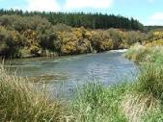
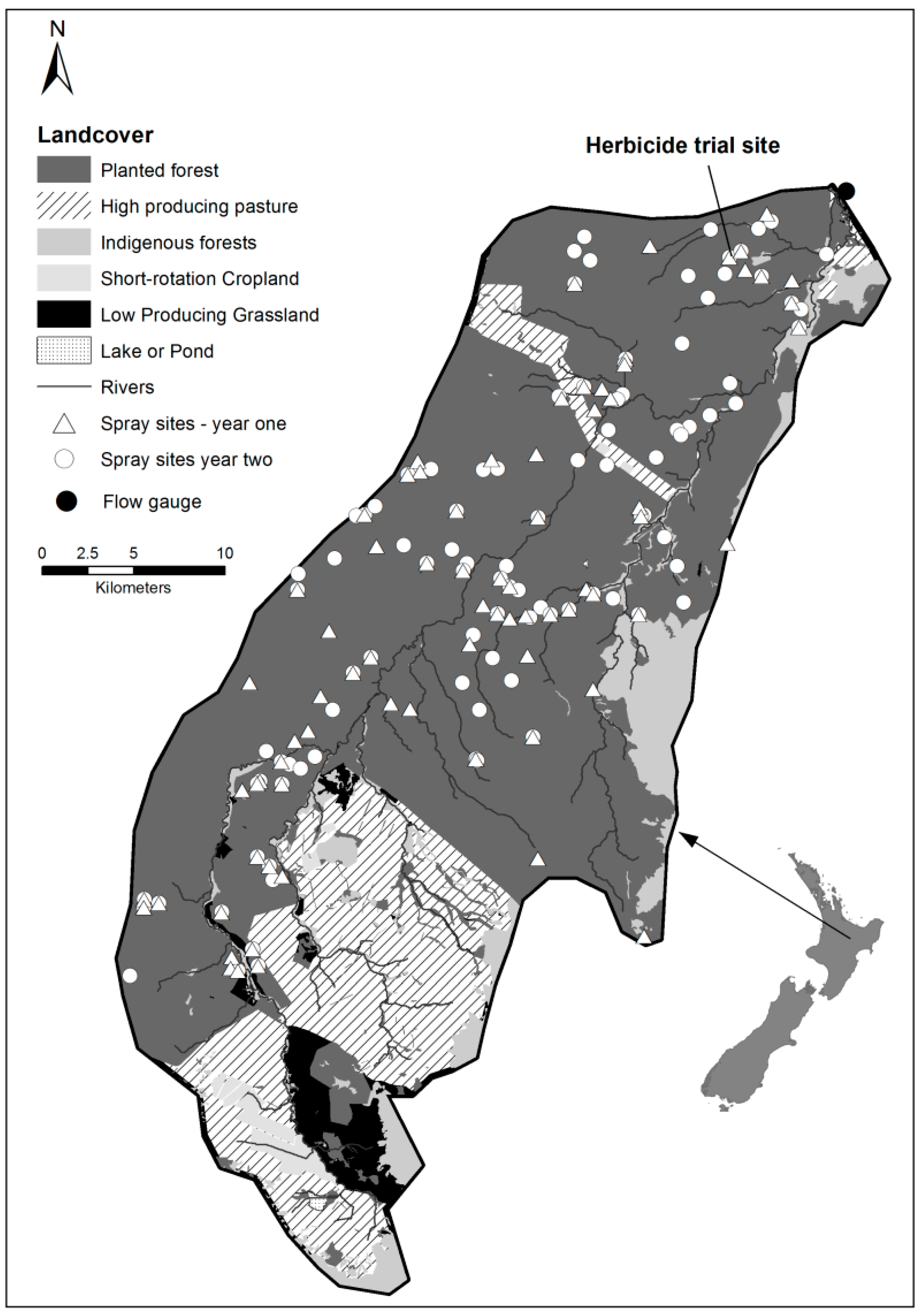
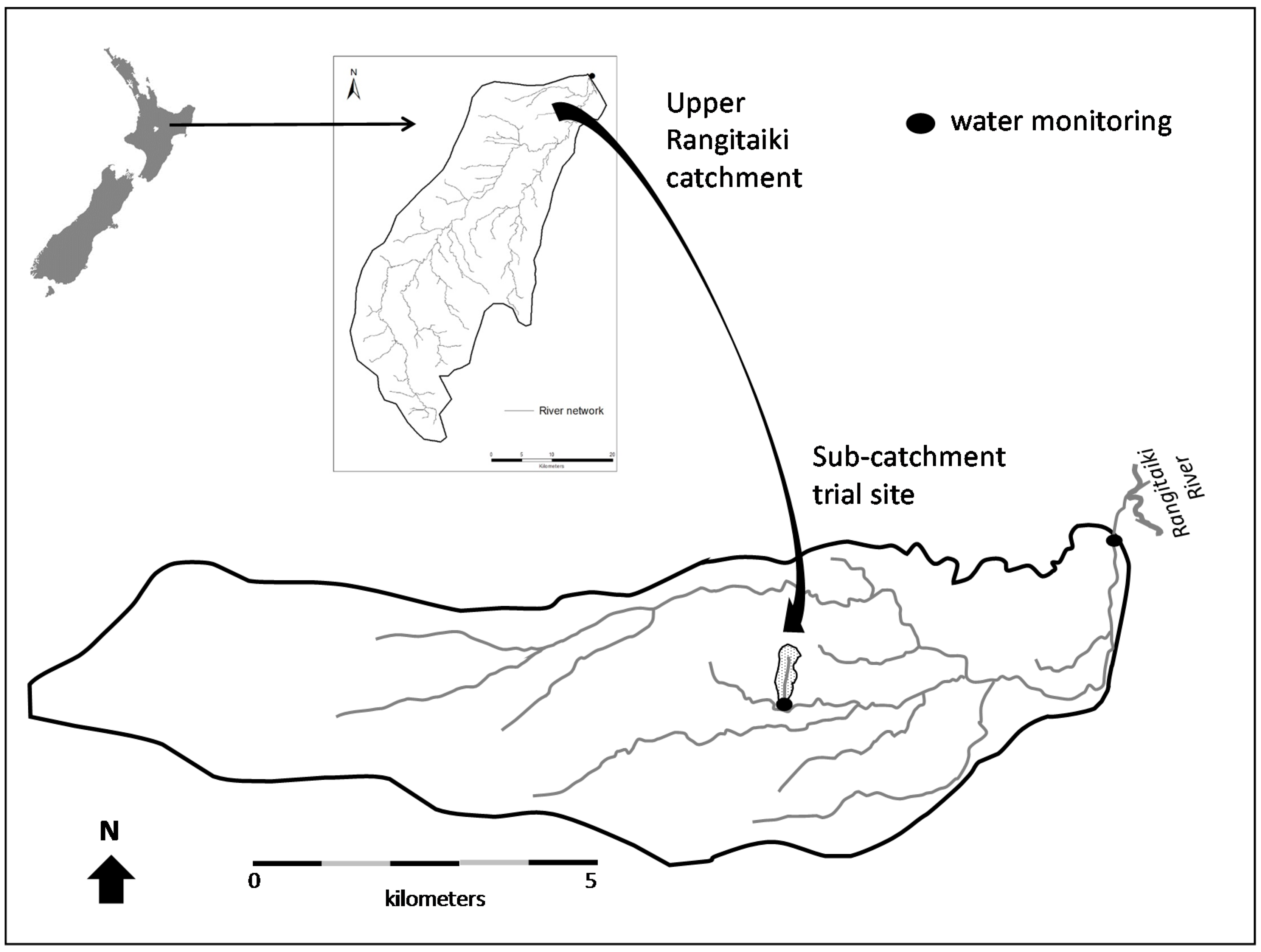
2.1. Study Catchment
2.2. Data Bases Used in the Cumulative Effects Model
2.2.1. Herbicide Trial
2.2.2. Herbicide Treatment Programme
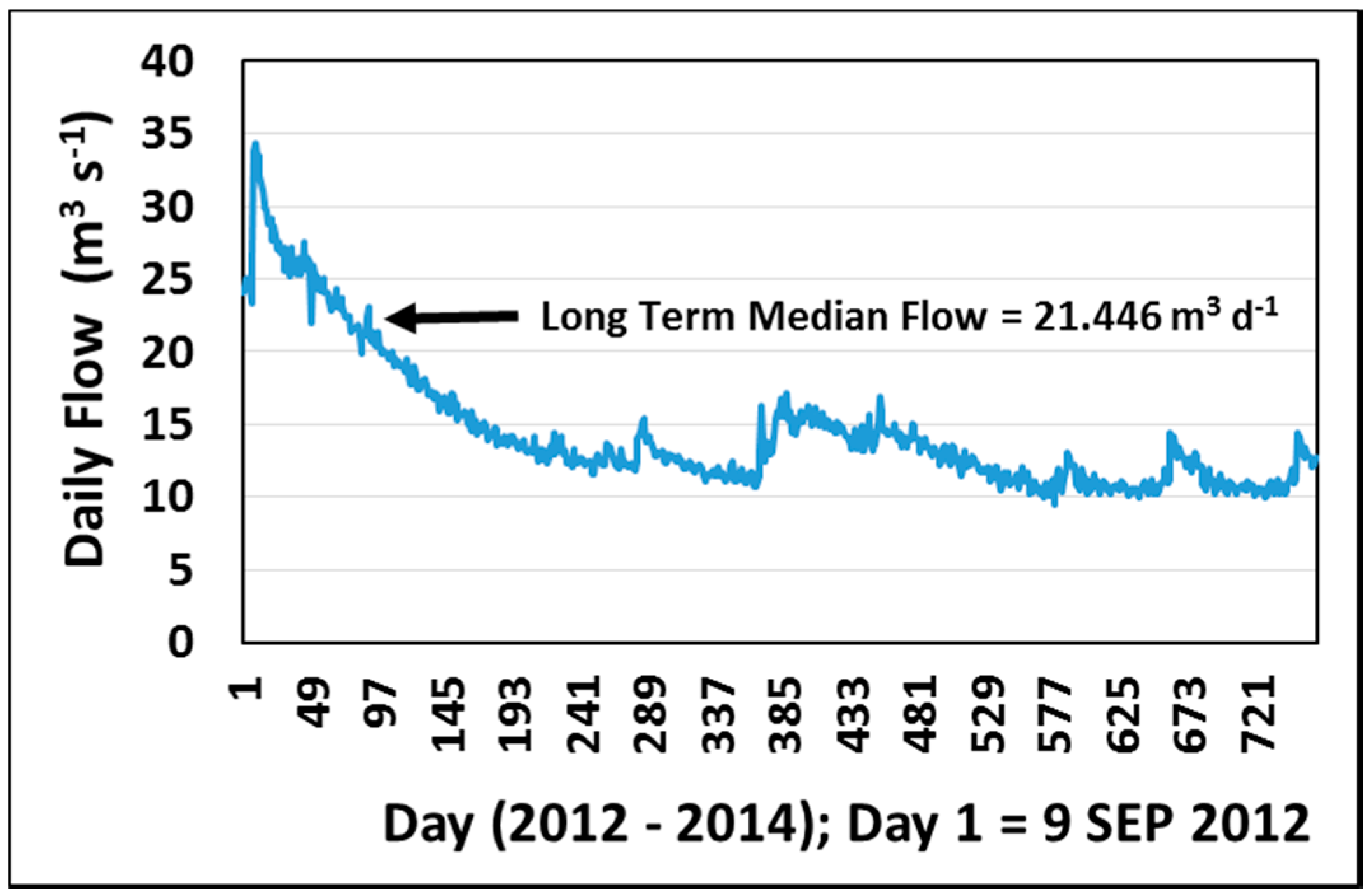
2.2.3. Flow Data
2.2.4. Herbicide Residue Analysis
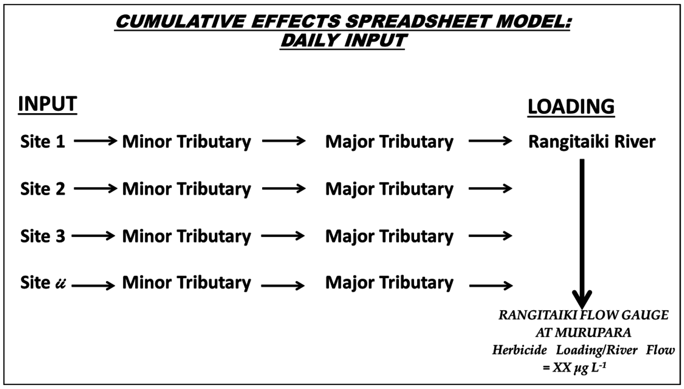
2.3. Model and Assumptions
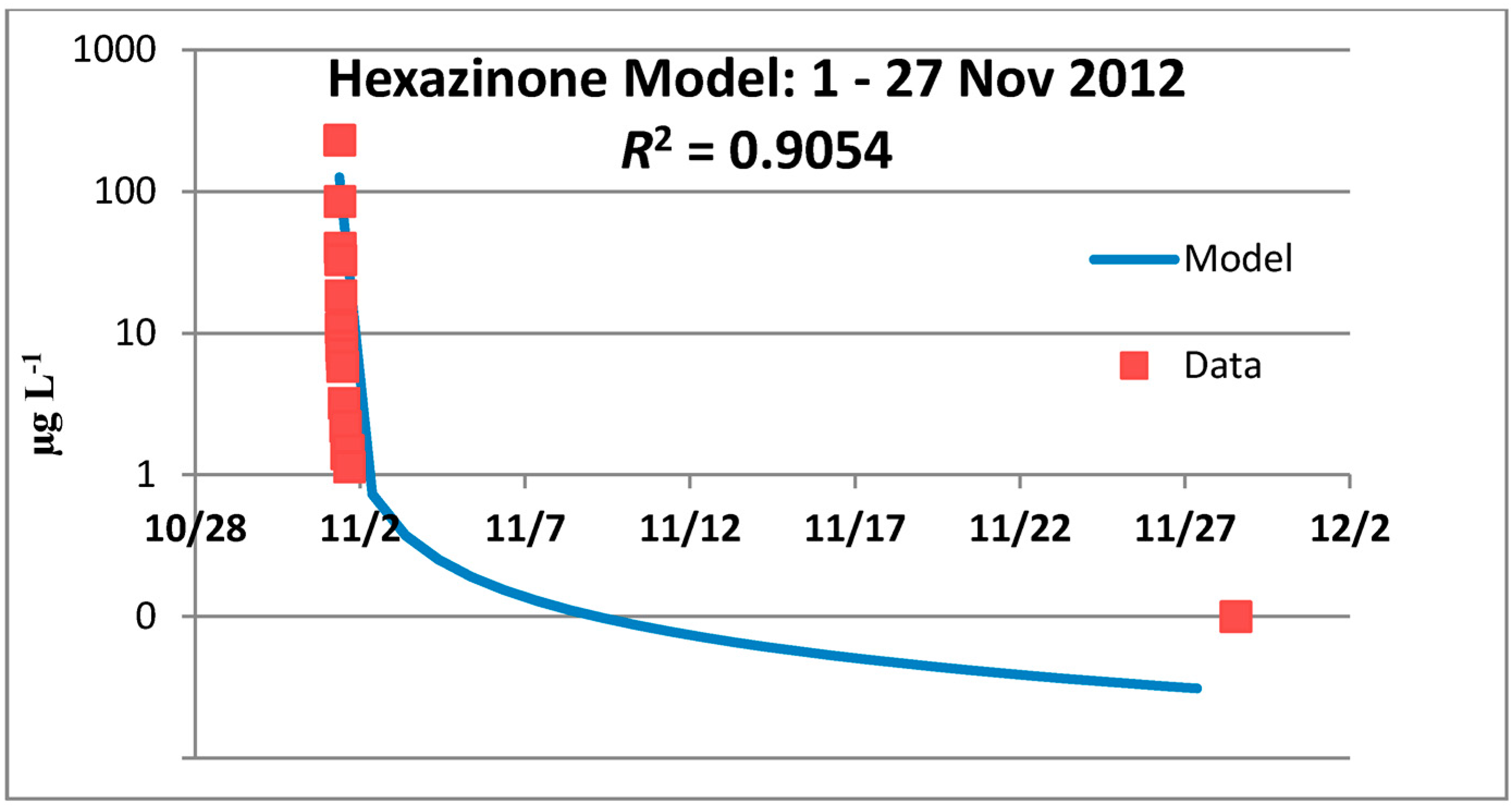
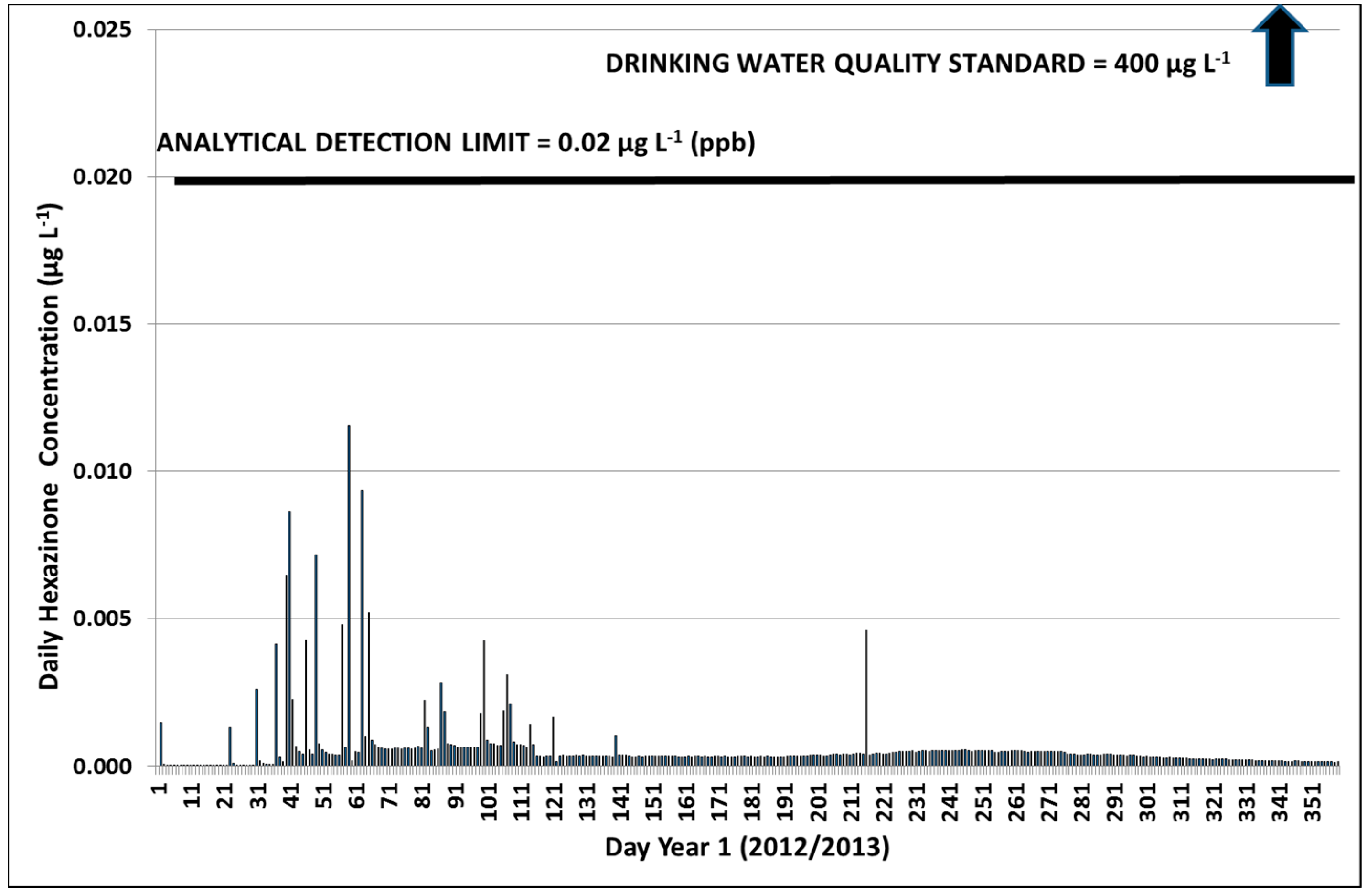
- x = time and date
- y = hexazinone concentration in μg·L−1.
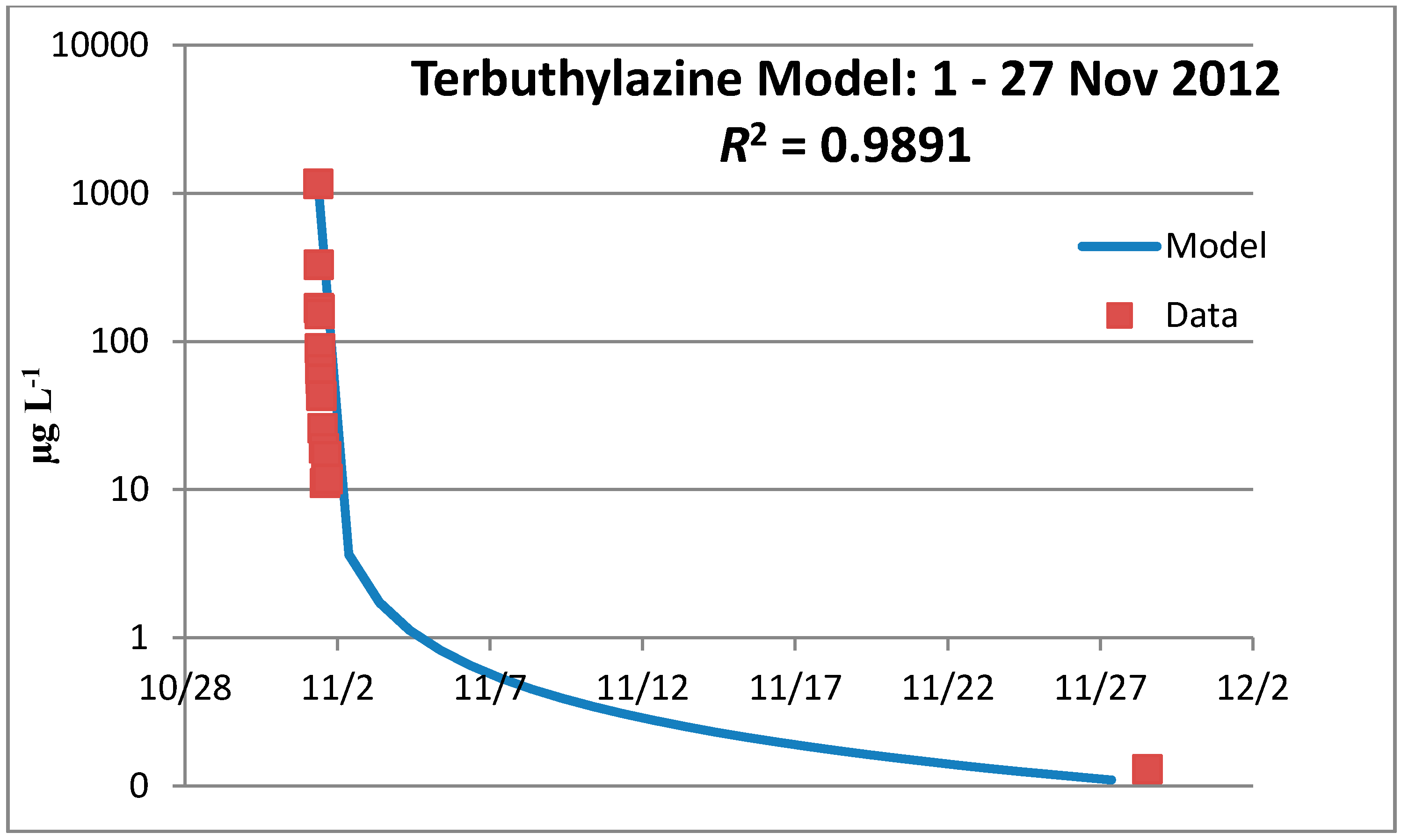
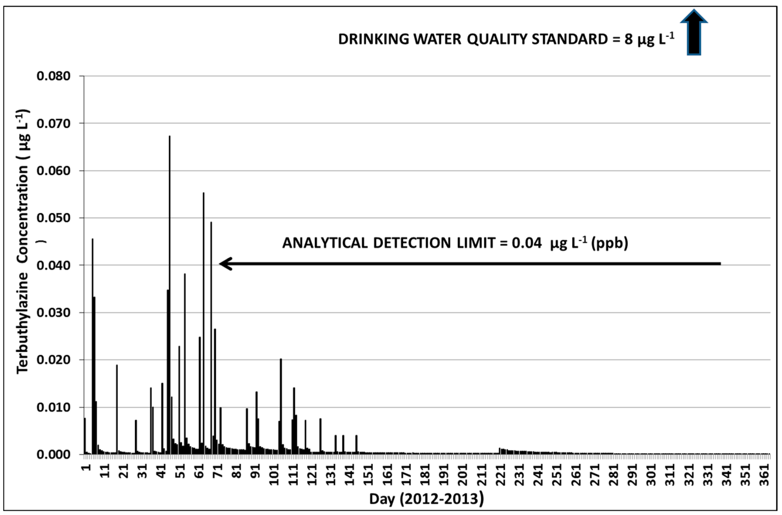
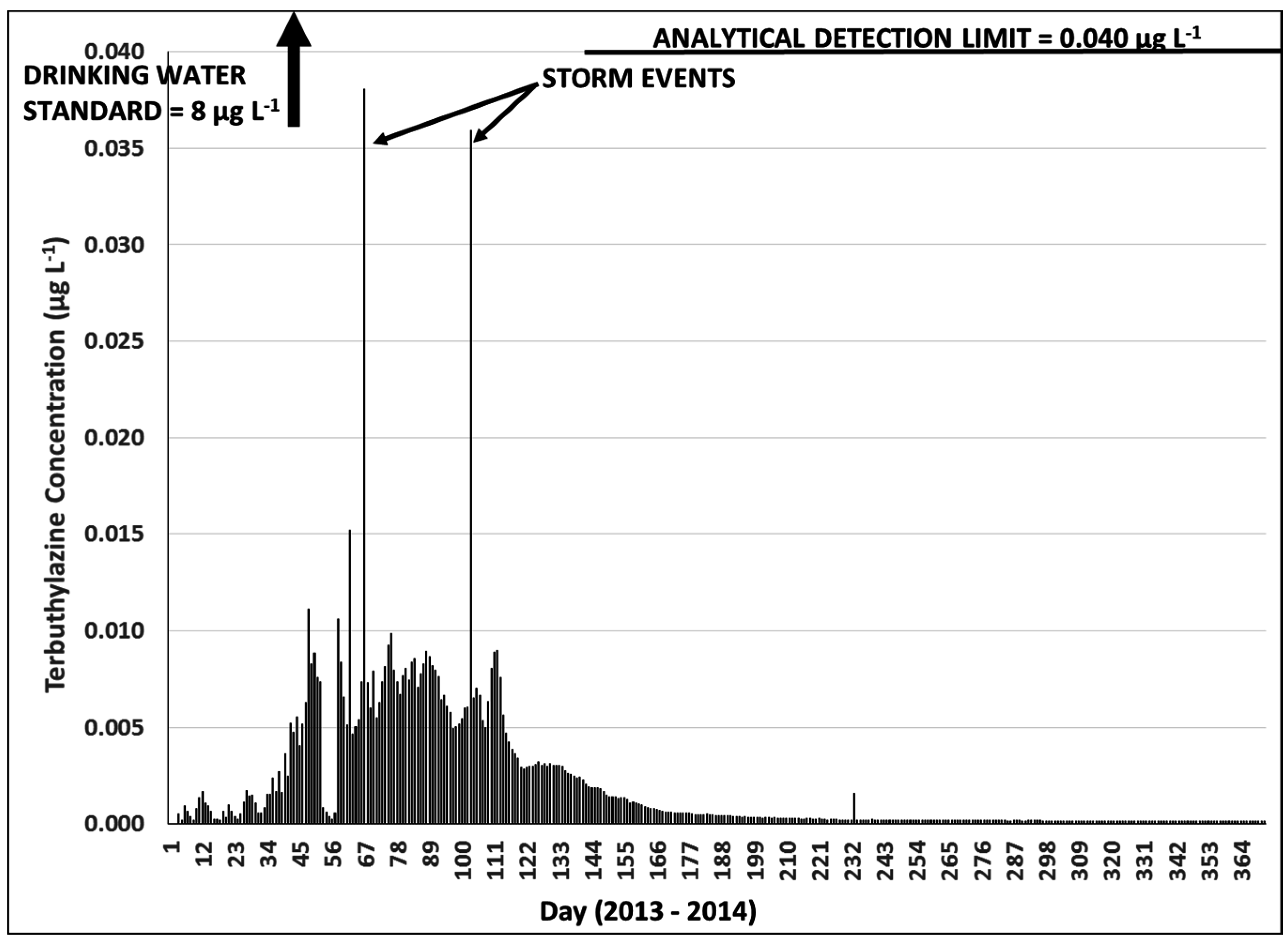
- x = time and date
- y = terbuthylazine concentration in μg·L−1.
2.4. Herbicide Degradation
3. Results
3.1. The Year 1 and Year 2 Spatial and Time Distributions of Herbicide Application
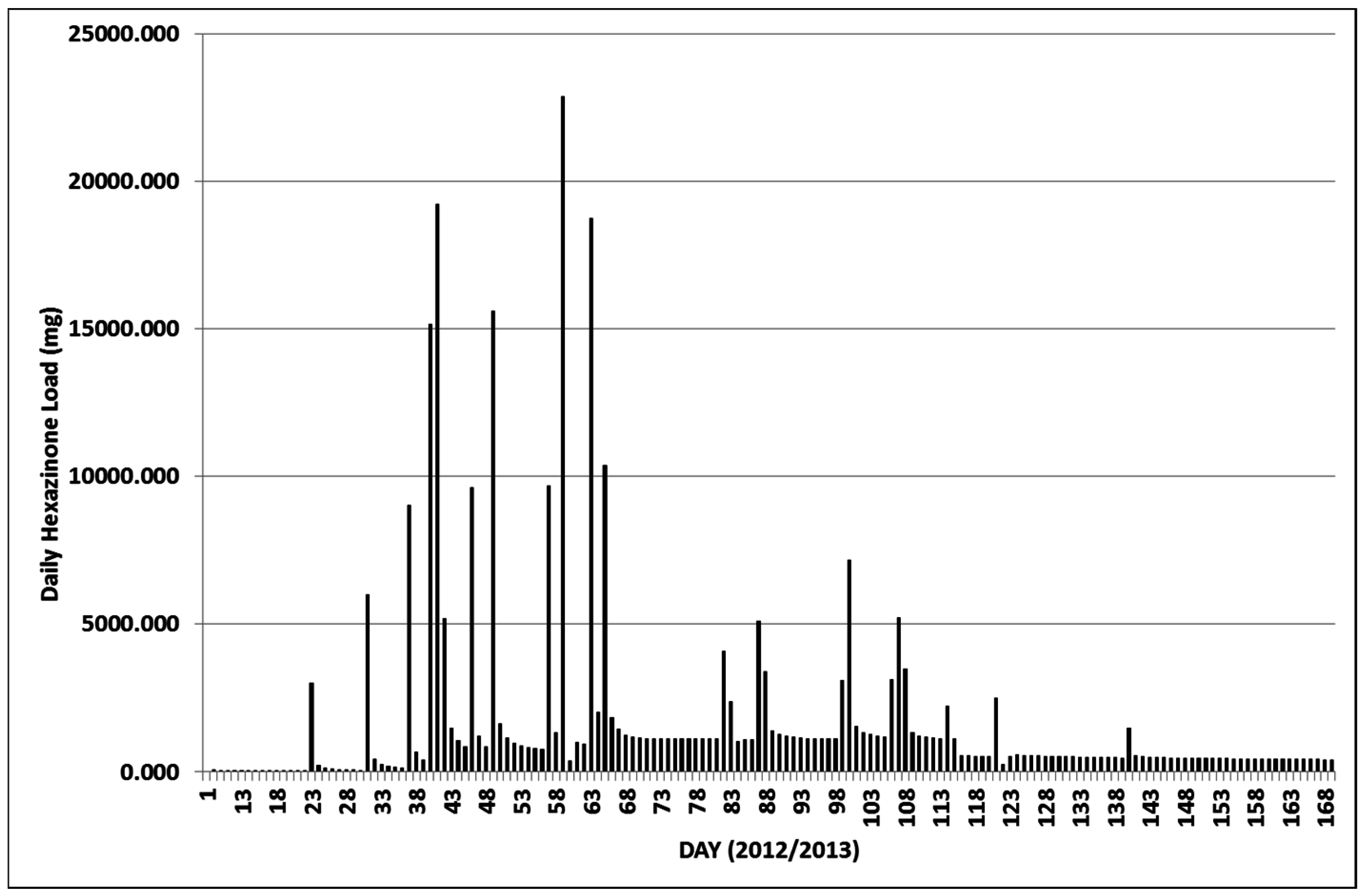
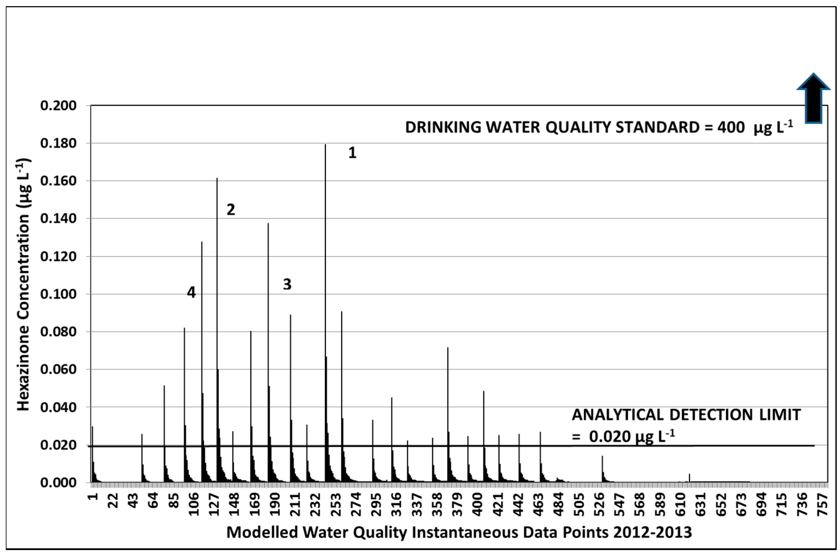
3.2. Hexazinone Cumulative Effects Analysis
3.2.1. Year 1
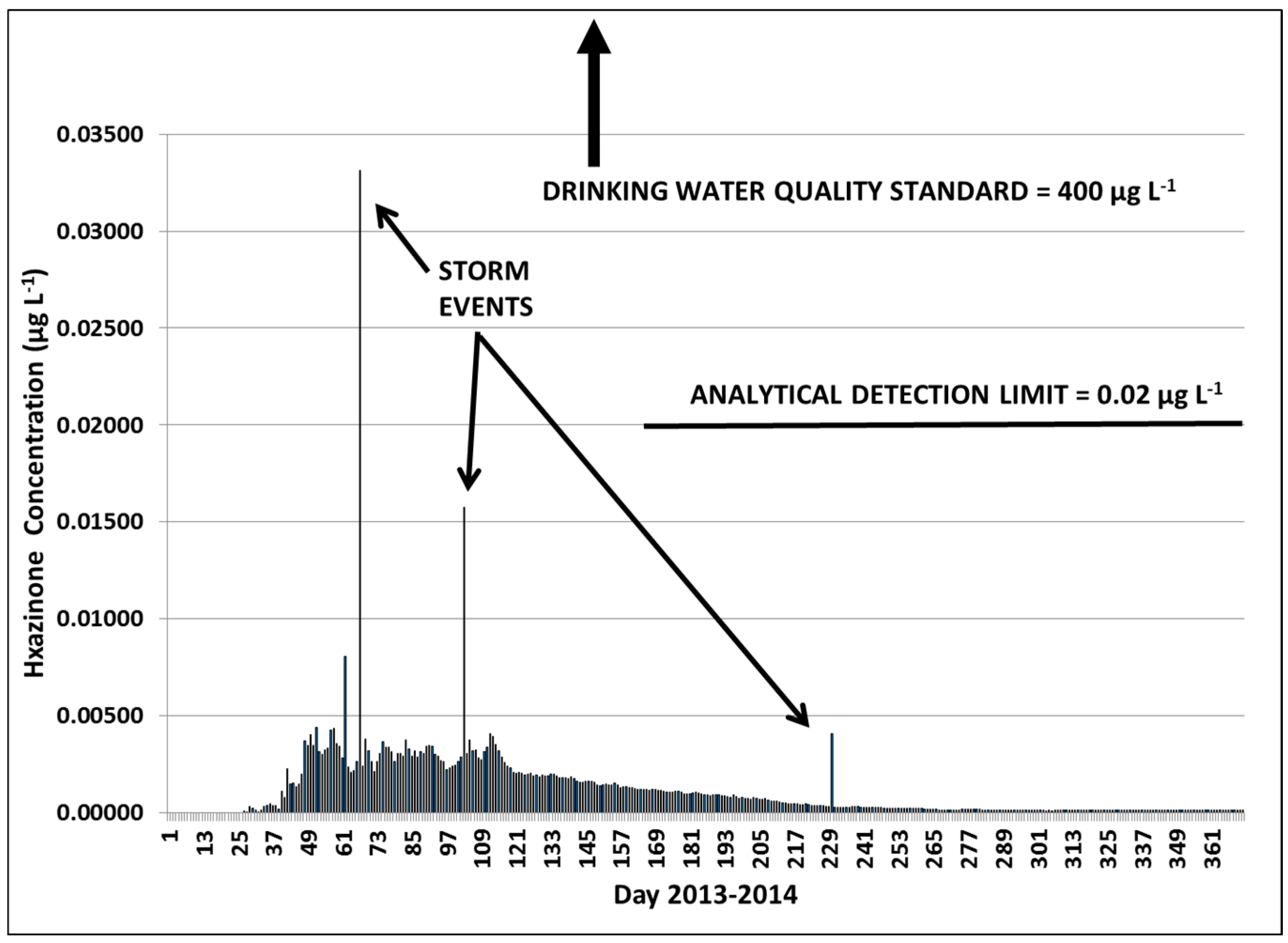
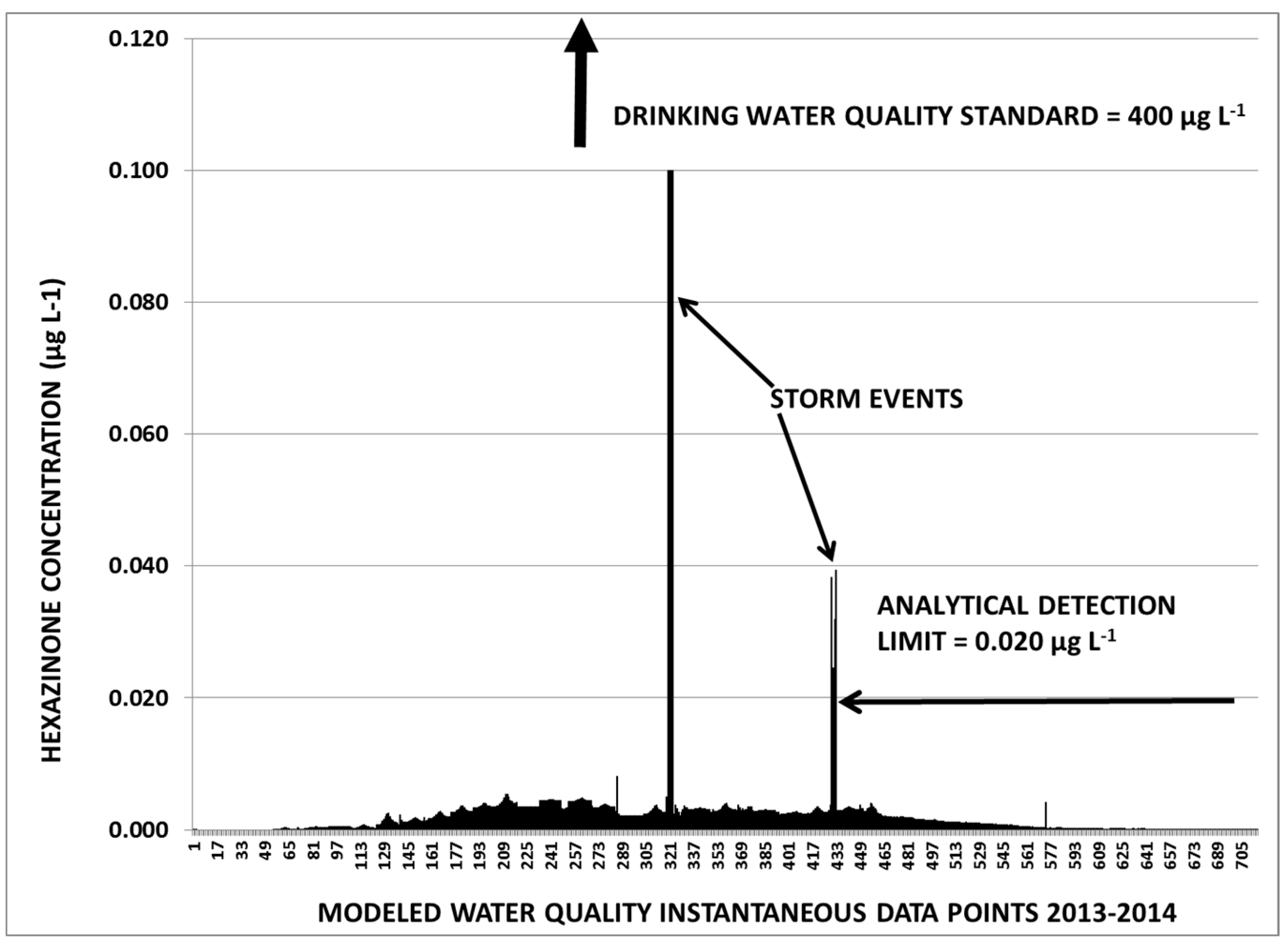
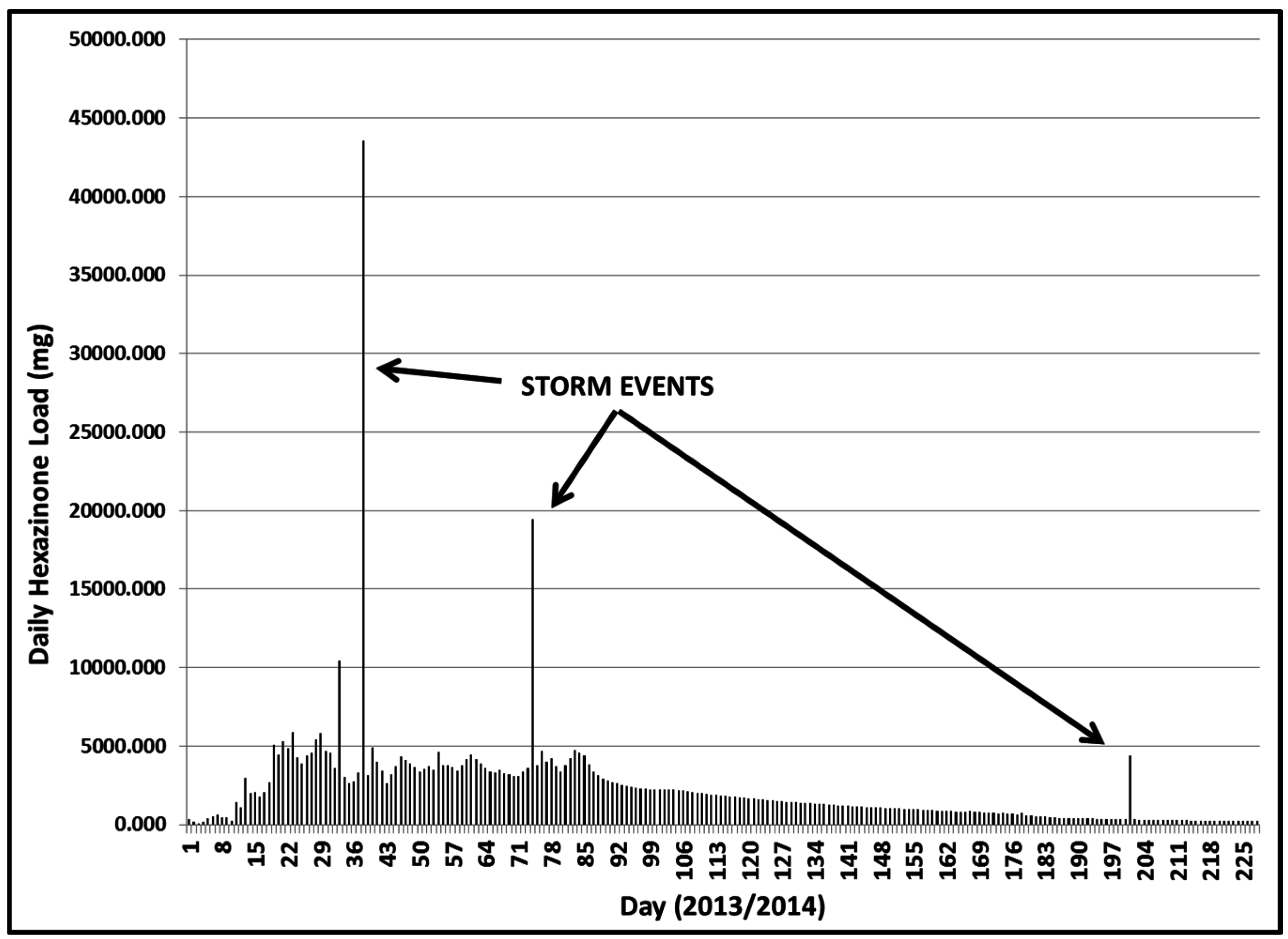
3.2.2. Year 2
3.2.3. Hexazinone Safety Factors
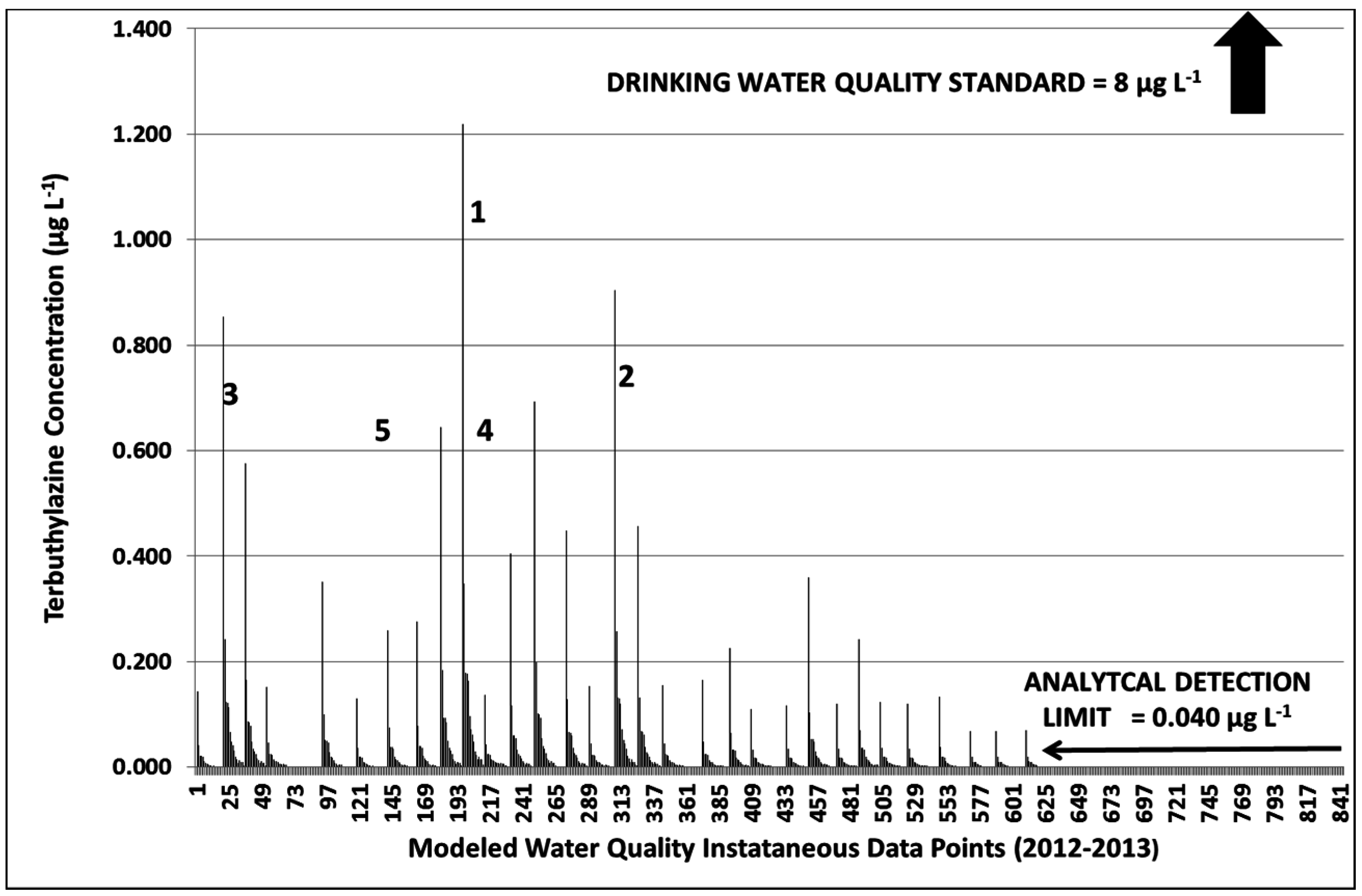
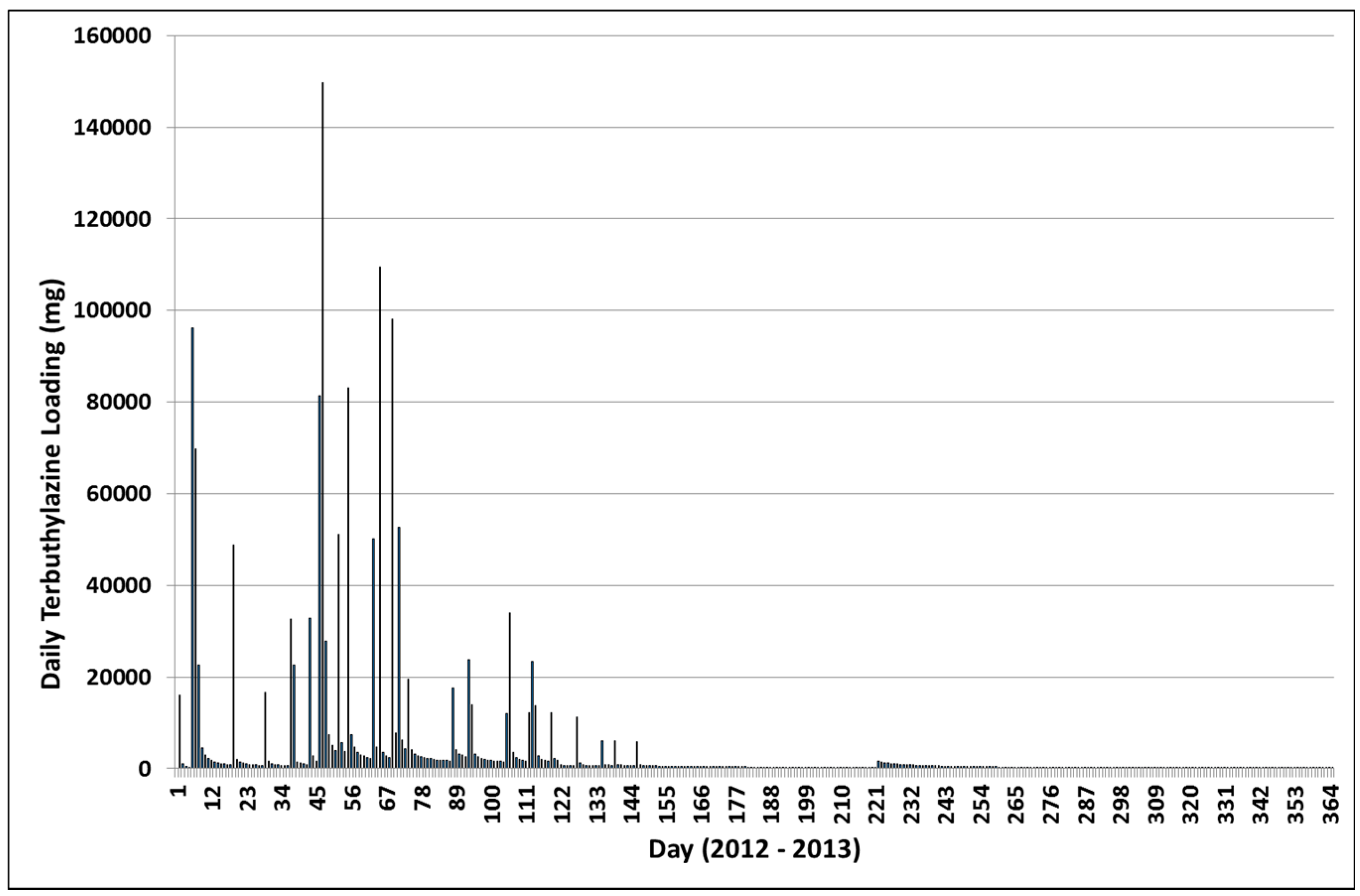
3.3. Terbuthylazine Cumulative Effects Analysis
3.3.1. Year 1
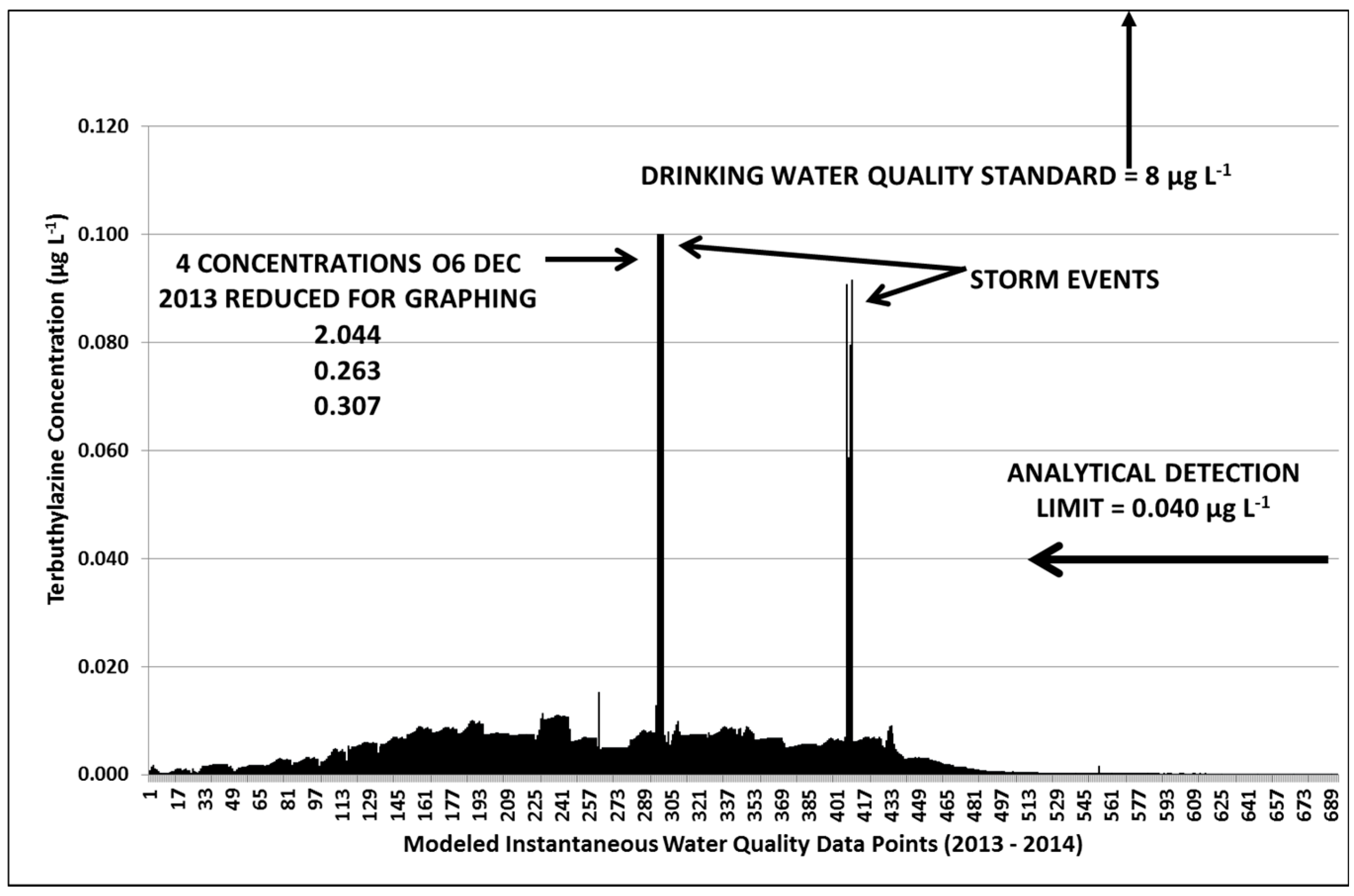
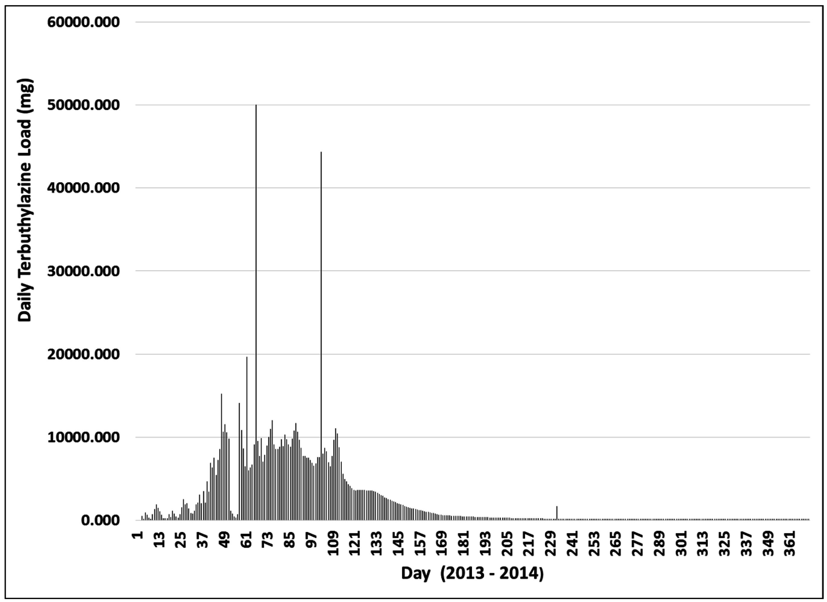
3.3.2. Year 2
3.3.3. Terbuthylazine Safety Factors
4. Discussion
5. Conclusions
Acknowledgments
Author Contributions
Conflicts of Interest
References
- Scatena, F.N. Drinking water quality. In Drinking Water from Forests and Grasslands: A Synthesis of the Scientific Literature; Dissmeyer, G.E., Ed.; General Technical Report SRS-39; USDA Forest Service Southern Research Station: Asheville, NC, USA, 2000; Chapter 2; pp. 7–25. [Google Scholar]
- Bolstad, P.V.; Swank, W.T. Cumulative impacts of land use on water quality in a southern Appalachian watershed. J. Am. Water Resour. Assoc. 1997, 33, 519–533. [Google Scholar] [CrossRef]
- Swanson, F.J.; Scatena, F.N.; Dissmeyer, G.E.; Fenn, M.E.; Verry, E.S.; Lynch, J.A. Watershed processes—Fluxes of water, dissolved constituents, and sediment. In Drinking Water from Forests and Grasslands: A Synthesis of the Scientific Literature; Dissmeyer, G.E., Ed.; General Technical Report SRS-39; USDA Forest Service Southern Research Station: Asheville, NC, USA, 2000; Chapter 3; pp. 26–41. [Google Scholar]
- Neary, D.G.; Ice, G.G.; Jackson, C.R. Linkages between forest soils and water quantity and quality. For. Ecol. Manag. 2009, 258, 2269–2281. [Google Scholar] [CrossRef]
- Neary, D.G. Experimental Forest Catchment Studies Contributions to the Understanding of the Effects of Disturbances on Water Quality: Past, Present, and Future. Available online: https://arizona.openrepository.com/arizona/bitstream/10150/301298/1/hwr_42-061-076.pdf (accessed on 21 November 2016).
- Dissmeyer, G.E. (Ed.) Drinking Water from Forests and Grasslands. A Synthesis of the Scientific Literature; General Technical Report SRS-39; USDA Forest Service Southern Research Station: Asheville, NC, USA, 2000; p. 246.
- Foley, J.A.; DeFries, R.; Asner, G.P.; Barford, C.; Bonan, G.; Carpenter, S.R.; Chapin, F.S.; Coe, M.T.; Daily, G.C.; Gibbs, H.K.; et al. Global consequences of land use. Science 2005, 309, 570–574. [Google Scholar] [CrossRef] [PubMed]
- Baillie, B.R.; Neary, D.G. Water quality in New Zealand’s planted forests: A review. N. Z. J. For. Sci. 2015, 45. [Google Scholar] [CrossRef]
- Larned, S.T.; Scarsbrook, M.R.; Snelder, T.H.; Norton, N.J.; Biggs, B.J.F. Water quality in low-elevation streams and rivers in New Zealand: Recent state and trends in contrasting land-cover classes. N. Z. J. Mar. Freshw. Res. 2004, 38, 347–366. [Google Scholar] [CrossRef]
- Little, K.M.; Willoughby, I.; Wagner, R.G.; Adams, P.; Frochot, H.; Gava, J.; Gous, S.; Lautenschlager, R.A.; Örlander, G.; Sankaran, K.V.; et al. Towards reduced herbicide use in forest vegetation management. South Afr. For. J. 2006, 207, 63–79. [Google Scholar] [CrossRef]
- Neary, D.G.; Bush, P.B.; Douglass, J.E. Offsite movement of hexazinone in stormflow and baseflow from forest watersheds. Weed Sci. 1983, 31, 543–551. [Google Scholar]
- Neary, D.G.; Bush, P.B.; Grant, M.A. Water quality of ephemeral forest streams after site preparation with the herbicide hexazinone. For. Ecol. Manag. 1986, 14, 23–40. [Google Scholar] [CrossRef]
- Neary, D.G. Effects of pesticide applications on forest watersheds. In Forest Hydrology and Ecology at Coweeta; Swank, W.T., Crossley, D.A., Jr., Eds.; Springer: New York, NY, USA, 1988; pp. 325–337. [Google Scholar]
- Neary, D.G.; Michael, J.J. Herbicides—Protecting long-term sustainability and water quality in forest ecosystems. N. Z. J. For. Sci. 1996, 26, 241–264. [Google Scholar]
- Rolando, C.A.; Garrett, L.G.; Baillie, B.R.; Watt, M.S. A survey of herbicide use and a review of environmental fate in New Zealand planted forests. N. Z. J. For. Sci. 2013, 43, 1–10. [Google Scholar] [CrossRef]
- Garrett, L.G.; Watt, M.S.; Rolando, C.A.; Pearce, S.H. Environmental fate of terbuthylazine and hexazinone in a New Zealand planted forest Pumice soil. For. Ecol. Manag. 2015, 337, 67–76. [Google Scholar] [CrossRef]
- Neary, D.G.; Bush, P.B.; Michael, J.L. Fate of pesticides in southern forests: A review of a decade of progress. Environ. Toxicol. Chem. 1993, 12, 411–428. [Google Scholar] [CrossRef]
- Fagg, P.C.; James, J.M.; Flinn, D.W.; Mainey, P. Residues of Hexazinone and Four of Its Metabolites in Stream Water after Aerial Spraying of a Pinus radiata Plantation near Yarram, Victoria; Forest Commission Victoria Report; Forest Commission: Victoria, Australia, 1982; p. 9.
- Leitch, C.J.; Flinn, D.W. Residues of hexazinone in streamwater after aerial application to an experimental catchment planted with radiata pine. Aust. For. 1983, 46, 126–131. [Google Scholar] [CrossRef]
- Skark, C.; Zullei-Seibert, N.; Uwe, W.; Gatzemann, U.; Schlett, C. Contribution of non-agricultural pesticides to pesticide load in surface water. Pest Manag. Sci. 2004, 60, 525–530. [Google Scholar] [CrossRef] [PubMed]
- Miller, J.H.; Bace, A.C., Jr. Streamwater Contamination after Aerial Application of a Pelletized Herbicide; Research Note SO-255; USDA Forest Service, Southern Forest Experiment Station: New Orleans, LA, USA, 1980; p. 4.
- Neary, D. Monitoring herbicide residues in springflow after an operational application of hexazinone. South. J. Appl. For. 1983, 7, 217–223. [Google Scholar]
- Neary, D.G.; Bush, P.B.; Douglass, J.E.; Todd, R.L. Picloram movement in an Appalachian forest watershed. J. Environ. Qual. 1985, 14, 585–592. [Google Scholar] [CrossRef]
- Lavy, T.L.; Mattice, J.D.; Kochenderfer, J.N. Hexazinone persistence and mobility of a steep forested watershed. J. Environ. Qual. 1984, 18, 507–514. [Google Scholar] [CrossRef]
- Bouchard, D.C.; Lavy, T.L.; Lawson, E.R. Mobility and persistence of hexazinone in a forest watershed. J. Environ. Qual. 1985, 14, 229–233. [Google Scholar] [CrossRef]
- Michael, J.L.; Neary, D.G. Herbicide dissipation studies in southern forest ecosystems. Environ. Toxicol. Chem. 1993, 12, 405–410. [Google Scholar] [CrossRef]
- Neary, D.G.; Michael, J.L.; Wells, M.J.M. Fate of hexazinone and picloram after herbicide site preparation in a cut-over northern hardwood forest. In Proceedings of the 1984 Annual Lake States Forest Soils Conference, L’Anse, MI, USA, 26–28 September 1984; pp. 55–72.
- Fiore, H. Water Monitoring Report: 1992 Herbicide Application Projects: Eldorado National Forest; USDA Forest Service, Eldorado National Forest: Placerville, CA, USA, 1992; p. 27.
- McBroom, M.W.; Louch, J.; Beasley, S.R.; Chang, M.; Ice, G.G. Runoff of silvicultural herbicides applied using best management practices. For. Sci. 2013, 59, 197–210. [Google Scholar] [CrossRef]
- Baillie, B.R.; Neary, D.G.; Gous, S. Aquatic fate of aerially applied hexazinone and terbuthylazine in a New Zealand planted forest. J. Sustain. Watershed Sci. Manag. 2015, 2, 118–129. [Google Scholar] [CrossRef]
- Boyle, J.R.; Wariloa, J.E.; Beschta, R.L.; Reiter, M.; Chambers, C.C.; Gibson, W.P.; Gregory, S.V.; Grizzel, J.; Hagar, J.C.; Li, J.L.; et al. Cumulative effects of forestry practices: An example framework for evaluation from Oregon, USA. Biomass Bioenergy 1997, 13, 223–245. [Google Scholar] [CrossRef]
- National Environmental Policy Act of 1969. Available online: https://www.fws.gov/r9esnepa/relatedlegislativeauthorities/nepa1969.pdf (accessed on 21 November 2016).
- Spaling, H. Cumulative effects assessment: Concepts and principles. Impact Assess. 1994, 12, 231–251. [Google Scholar] [CrossRef]
- Holling, C.S. Resilience and stability of ecological systems. Annu. Rev. Ecol. Syst. 1973, 4, 1–23. [Google Scholar] [CrossRef]
- Barrett, G.W.; Van Dyn, G.M.; Odum, E.P. Stress ecology. Bioscience 1976, 26, 192–194. [Google Scholar] [CrossRef]
- Barrett, G.W.; Rosenberg, R. (Eds.) Stress Effects on Natural Ecosystems; John Wiley: Chichester, UK; New York, NY, USA, 1976; p. 305.
- Therivel, R.; Ross, B. Cumulative effects assessment—Does scale matter. Environ. Impact Asses. Rev. 2007, 27, 365–385. [Google Scholar] [CrossRef]
- Neary, D.G.; Smethurst, P.J.; Baillie, B.; Petrone, K.C. Water Quality, Biodiversity, and Codes of Practice in Relation to Harvesting Forest Plantations in Streamside Management Zones; Commonwealth Scientific and Industrial Research Organization Special Report; Commonwealth Scientific and Industrial Research Organization: Canberra, Australia, 2011; p. 99. [Google Scholar]
- Bennett, G.W.; Chorley, R.J. Environmental Systems: Philosophy, Analysis and Control; Princeton University Press: Princeton, NJ, USA, 1978; p. 624. [Google Scholar]
- Rapport, D.J.; Regier, H.A.; Hutchinson, T.C. Ecosystem behavior under stress. Am. Nat. 1985, 125, 617–640. [Google Scholar] [CrossRef]
- Sarmah, A.K.; Müller, K.; Ahmad, R. Fate and behavior of pesticides in the agroecosystem—A review with a New Zealand perspective. Aust. J. Soil Res. 2004, 42, 125–154. [Google Scholar] [CrossRef]
- Beanlands, G.E.; Policansky, D.; Erckmann, W.J.; Sadar, M.H.; Orians, G.H.; O’Riordan, J. (Eds.) Cumulative Environmental Effects: A Binational Perspective; The Canadian Environmental Assessment Research Council: Ottawa, ON, Canada; The United States National Research Council: Washington, DC, USA, 1986.
- Orians, G.H. Opening discussions—Cumulative effects: Setting the stage. In Cumulative Environmental Effects: A Binational Perspective; Beanlands, G.E., Policansky, D., Erckmann, W.J., Sadar, M.H., Orians, G.H., O’Riordan, J., Eds.; The Canadian Environmental Assessment Research Council: Ottawa, ON, Canada; The United States National Research Council: Washington, DC, USA, 1986; p. 175. [Google Scholar]
- Molloy, L. Soils in the New Zealand Landscape: The Living Mantle, 2nd ed.; New Zealand Society of Soil Science: Canterbury, New Zealand, 1998. [Google Scholar]
- Leonard, G.S.; Begg, J.G.; Wilson, C.J.N. (Comps.). Geology of the Rotorua Area: Institute of Geological & Nuclear Sciences 1:250,000 Geological Map 5. 1 Sheet + 102p; GNS Science: Lower Hutt, New Zealand, 2010. [Google Scholar]
- Holdridge, L.R. Life Zone Ecology; Tropical Science Center: San Jose, Costa Rica, 1967; p. 206. [Google Scholar]
- Quayle, A.M. The Climate and Weather of the Bay of Plenty Region; New Zealand Meteorological Service, Ministry of Transport: Wellington, New Zealand, 1984; p. 56.
- Thompson, C.S. The Weather and Climate of the Tongariro Region; New Zealand Meteorological Service, Ministry of Transport: Wellington, New Zealand, 1984.
- Climatemps. 2014. Available online: http://www.murupara.climatemps.com/ (accessed on 24 November 2014).
- Porteous, A.; Mullan, B. The 2012–2013 Drought: An Assessment and Historical Perspective; Ministry of Primary Industries Technical Paper No: 2012/18; NIWA: Wellington, New Zealand, 2013; p. 57. [Google Scholar]
- U.S. Environmental Protection Agency. Available online: http://www.epa.gov/osw/hazard/testmethods/sw846/pdfs/3510c.pdf (accessed on 21 November 2016).
- EXCEL Spreadsheet Software. Available online: https://www.microsoftstore.com/US/Microsoft_Excel (accessed on 15 January 2015).
- Maptoaster Topo© Version 6 Integrated Mapping. 2015. Available online: https://www.maptoaster.com/maptoaster-topo-nz/index.html (accessed on 15 January 2015).
- Richardson, B.; Ray, J.; Vanner, A.; Davenhill, N.; Miller, K. Nozzles for minimising aerial herbicide spray drift. N. Z. J. For. Sci. 1996, 26, 438–448. [Google Scholar]
- New Zealand Ministry of Health. Drinking Water Standards for New Zealand 2005 (Revised 2008); Ministry of Health: Wellington, New Zealand, 2008.
- World Health Organization. Terbuthylazine (TBA) in Drinking Water: Background Document for Development of WHO Guidelines for Drinking Water Quality; World Health Organization: Genera, Switzerland, 2003. [Google Scholar]
- Watt, M.S.; Rolando, C.A.; Zaayman, M.; Martin, K. Adsorption of the herbicide terbuthylazine across a range of New Zealand forestry soils. Can. J. For. Res. 2010, 40, 1448–1457. [Google Scholar] [CrossRef]
- Ghassemi, M.; Fargo, L.; Painter, P.; Quinlivan, S.; Schofield, R.; Takata, A. Environmental fates and impacts of major forest use pesticides. In Environmental Fates and Impacts of Major Forest Use Pesticides; TRW: Redondo Beach, FL, USA; U.S. EPA Office of Pesticides and Toxic Substances: Washington, DC, USA, 1981; pp. A169–A194. [Google Scholar]
- Durkin, P.; King, C.; Klotzbach, J. Hexazinone—Human Health and Ecological Risk Assessment—Final Report; Syracuse Environmental Research Associates, Inc.: Fayetteville, NY, USA, 2005; p. 281. [Google Scholar]
- Rhodes, R.C. Studies with “Velpar” Weed Killer in Water; Document No. AB29645E; DPR# 369-039; E.I. du Pont de Nemours and Co., Inc.: Wilmington, DE, USA, 1986; Unpublished study. [Google Scholar]
- Wang, H.; Lin, K.; Hou, Z.; Richardson, B.; Gan, J. Sorption of the herbicide terbuthylazine in two New Zealand forest soils amended with biosolids and biochars. J. Soils Sediments 2010, 10, 283–289. [Google Scholar] [CrossRef]
- Palm, W.U.; Zetzsch, C. Investigation of the photochemistry and quantum yields of triazines using polychromatic irradiation and UV-spectroscopy as analytical tools. Int. J. Environ. Anal. Chem. 1996, 65, 313–329. [Google Scholar] [CrossRef]
- World Health Organizaion. Guidelines for Drinking-Water Quality, 4th ed.; WHO: Geneva, Switzerland, 2011; p. 564. [Google Scholar]
- Webb, A.A.; Bonell, M.; Bren, L.; Lane, P.N.J.; McGuire, D.; Neary, D.G.; Nettles, J.; Scott, D.F.; Stednick, J.D.; Wang, Y. Revisiting experimental catchment studies in forest hydrology. In Proceedings of the 2011 International Union of Geodesy and Geophysics XXV General Assembly, Melbourne, Australia, 6–8 July 2011; p. 234.
- Smith, D.G.; Ruurd Maasdam, R. New Zealand’s national river water quality network 1. Design and physic-chemical characterization. N. Z. J. Mar. Freshw. Res. 1994, 28, 19–35. [Google Scholar] [CrossRef]
- Land Air Water Aotearoa. Rangitaiki River at Old Bridge at Murupara. 2015. Available online: http://www.lawa.org.nz/explore-data/bay-of-plenty-region/rangitaiki-river/rangitaiki-river-at-old-bridge-at-murupara/ (accessed on 28 November 2014).
- Staudenmayer, H.; Selner, J.C. Failure to assess psychopathology in patients presenting with chemical sensitivities. J. Occup. Environ. Med. 1995, 37, 704–709. [Google Scholar] [CrossRef] [PubMed]
- Das-Munshi, J.; Rubin, G.J.; Wessely, S. Multiple chemical sensitivities: A systematic review of provocation studies. J. Allergy Clin. Immun. 2006, 118, 1257–1264. [Google Scholar] [CrossRef] [PubMed]
- Close, M.E.; Skinner, A. Sixth national survey of pesticides in groundwater in New Zealand. N. Z. J. Mar. Freshw. Res. 2012, 46, 443–457. [Google Scholar] [CrossRef]


| Type | Characteristics | Examples |
|---|---|---|
| Time Crowding | Frequent and repetitive activities in the same time frame | Multiple herbicide applications within a catchment the same day |
| Space Crowding | Management activities on the same sites | Harvesting, site preparation, burning, and chemical applications on the same stand |
| Synergistic | Effects from different activities that multiply the impact | Multiplicative effects of herbicides or fertilizers on vegetation & water quality |
| Indirect | Secondary effects not directly related to an activity | Nitrogen release into groundwater after harvesting mature stands |
| Nibbling | Incremental reductions in water quality | Changes in water quality from inputs of pollutants along a stream course |
| Time Lag | Time-delayed effects from land management activities | Delayed movement of fertilizers or herbicide residues into streams |
| Cross-Boundary | Impacts occurring away from the site of the activity | Chemical drift from fertilized paddocks into forested areas |
| Trigger/Threshold | Changes in system behavior and characteristics | Global climate change, drought, tropical cyclones |
| Fragmentation | Change in land use the breaks up continuity of an ecosystem | Urbanization of forest lands or conversions to agriculture |
| Year | Sites (No.) | Herbicide # | Area Range (ha) | Prescribed Rate (L·ha−1) |
|---|---|---|---|---|
| 1 | 63 | Release KT™ | 3.9–172.3 | 15–17 |
| 21 | Gardoprim™ | 3.1–78.0 | 15 | |
| 1 | Gardoprim™ and Viper 90DF™ | 31.3 | 15 & 1 * | |
| 1 | Viper 90DF™ | 100.8 | 1 * | |
| 2 | 83 | Release KT™ | 2.8–120.5 | 15–17 |
| 7 | Release KT™ and Viper 90DF™ | 2.6–44.3 | 15–17 & 1 * | |
| 2 | Release KT™ and Gardoprim™ | 24.5–53.0 | 15 | |
| 12 | Gardoprim™ | 6.6–136.8 | 15 | |
| 1 | Gardoprim™ and Viper 90DF™ | 189.4 | 1 * | |
| 3 | Viper 90DF™ | 1.6–39.8 | 1 * |
| Herbicide Transit Time to the Rangitaiki Gauge (h) | Year 1 | Year 2 |
|---|---|---|
| No. of Sites | No. of Sites | |
| 0–5 | 8 | 17 |
| 5–10 | 10 | 19 |
| 10–15 | 25 | 33 |
| 15–20 | 22 | 15 |
| 20–25 | 6 | 5 |
| 25–30 | 6 | 6 |
| Parameter @ | Life Form | Standard @ | Ingestion/Exposure | Safety Factor | Safety Factor |
|---|---|---|---|---|---|
| Year 1 | Year 2 | ||||
| Human ADI # | 50 kg Adult | 0.25 mg·day−1 | 4 L·day−1 | >5410 | >1886 |
| Human ADI # | 50 kg Adult | 0.25 mg·day−1 | 1.0 m3·day−1 | >22 | >7 |
| New Zealand Drinking Water Standard | - | 400 μg·L−1 | Mean Daily Concentration | >34,623 | >12,074 |
| New Zealand Drinking Water Standard | - | 400 μg·L−1 | Instantaneous Concentration | >1861 | >4000 |
| Daphnia LC50 | Adult | >21,000 μg·L−1 | 48 h | >117,087 | >4.420 × 10⁶ |
| Oncorhynchus mykiss LC50 | Adult | 320,000 μg·L−1 | 96 h | >1.784 × 10⁶ | >3.200 × 10⁶ |
| Parameter @ | Life Form | Standard @ | Ingestion/Exposure # | Safety Factor | Safety Factor |
|---|---|---|---|---|---|
| Year 1 | Year 2 | ||||
| Human ADI # | 50 kg Adult | 0.20 mg·day−1 | 4 L·day−1 | >25,986 | >1711 |
| Human ADI # | 50 kg Adult | 0.20 mg·day−1 | 1.0 m3·day−1 | >104 | >7 |
| New Zealand Drinking Water Standard | - | 8 μg·L−1 | Mean Daily Concentration | >119 | >8 |
| New Zealand Drinking Water Standard | - | 8 μg·L−1 | Instantaneous Concentration | >7 | >80 |
| Daphnia LC50 | Adult | 442,000 μg·L−1 | 48 h | >362,510 | >216,234 |
| Oncorhynchus mykiss LC50 | Adult | 3800 μg·L−1 | 96 h | >3117 | >1859 |
| Year | Applications | Herbicide Applied | Time Crowding Occurrence | Space Crowding Occurrence |
|---|---|---|---|---|
| Calendar | Days | Days | Days | |
| 1 (2013) | 13 September–24 January | 26 | 17 | 8 |
| 2 (2014) | 4 September–13 December | 26 | 22 | 15 |
| Total Nitrogen (μg·L−3) | Total Phosphorus (μg·L−3) | Turbidity (NTU) | Bacteria (E. coli) No./100 mL | Peak Terbuthylazine (μg·L−3) | Peak Hexazinone (μg·L−3) |
|---|---|---|---|---|---|
| 1089.5 | 29.5 | 1.4 | 26 | 2.044 | 0.179 |
© 2016 by the authors; licensee MDPI, Basel, Switzerland. This article is an open access article distributed under the terms and conditions of the Creative Commons Attribution (CC-BY) license (http://creativecommons.org/licenses/by/4.0/).
Share and Cite
Neary, D.G.; Baillie, B.R. Cumulative Effects Analysis of the Water Quality Risk of Herbicides Used for Site Preparation in the Central North Island, New Zealand. Water 2016, 8, 573. https://doi.org/10.3390/w8120573
Neary DG, Baillie BR. Cumulative Effects Analysis of the Water Quality Risk of Herbicides Used for Site Preparation in the Central North Island, New Zealand. Water. 2016; 8(12):573. https://doi.org/10.3390/w8120573
Chicago/Turabian StyleNeary, Daniel G., and Brenda R. Baillie. 2016. "Cumulative Effects Analysis of the Water Quality Risk of Herbicides Used for Site Preparation in the Central North Island, New Zealand" Water 8, no. 12: 573. https://doi.org/10.3390/w8120573
APA StyleNeary, D. G., & Baillie, B. R. (2016). Cumulative Effects Analysis of the Water Quality Risk of Herbicides Used for Site Preparation in the Central North Island, New Zealand. Water, 8(12), 573. https://doi.org/10.3390/w8120573