Characteristics of Droughts in South Africa: A Case Study of Free State and North West Provinces

Abstract

The Free State (FS) and North West (NW) Provinces are often hard hit by droughts with impacts on water availability, farm production and livestock holdings. The South African government declared the two Provinces drought disaster areas in the 2015/2016 hydrological year. This is a major drawback, since both the Provinces play an important role to South African economy as they are a haven to agricultural production and have major water reservoirs in South Africa. This study was undertaken to investigate the historical evolution of drought within the FS and NW Provinces over the past 30 years. The Standardized Precipitation Index (SPI) and Standardized Precipitation Evapotranspiration Index (SPEI) calculated based on monthly meteorological data from 14 weather/climate stations within the FS and NW Provinces were used to explore and characterize variation in drought intensity, duration, frequency and severity in FS and NW Provinces during 1985–2015. Results indicate that there exist localized positive and negative trends with spatial dependence across the selected stations. In particular, about 60% of the weather stations exhibiting a decreasing trend are located in FS Province, suggesting that FS has being experiencing increasing drought during the analyzed period compared to NW Province. Results from the analysis of drought evaluation indicators (DEIs) calculated from SPEI suggest that drought severity and frequency was more pronounced in FS while the intensity of the drought was more in NW Province during 1985–2015. In addition, based on SPEI calculations, moderate drought occurrences increased during 1985–1994 and 1995–2004 periods and decreased thereafter (2005–2015) in both Provinces. Drought classification based on parameters derived from SPEI produced similar results for mild drought occurrences during the same time scales.

1. Introduction

Extreme Earth systems processes have continued to manifest in terms of natural hazards whose impacts are felt by the entire ecosystem including mankind. Drought is one such extreme physical process and is often characterized as a slow-onset natural hazard whose impacts are complex and reverberate through many sectors of the economy such as water resources, agriculture, and natural ecosystems [1,2]. Furthermore, there is a compelling body of knowledge that link droughts to other epidemics like famine, diseases and land degradation globally. The inherent characteristics and impacts of droughts on the ecosystem and society at large has made drought the subject of numerous studies (e.g., see [3,4,5,6] and references therein).

To this end, a precise, unequivocal definition of drought remains elusive. Various definitions of drought have been suggested in the literature, all relating to specific drought impacts on economic activities, ecosystems, and society and water management issues [7,8,9,10]. A review by Dracup et al. [7] and Wilhite and Glantz [8] alluded to drought as a condition of insufficient moisture caused by a deficit in precipitation over some time period. According to Pereira et al. [11], drought can be defined as a temporal imbalance of water availability consisting of a persistent lower than average precipitation of uncertain frequency, duration and unpredictable severity. In Vicente-Serrano et al. [2] and references therein, drought is described as a natural phenomenon which occurs when water availability is significantly below normal levels over a long period of time and cannot meet demand.

As reported in Halwatura et al. [12], drought periods can be characterized from a few hours (short-term) to millennia (long-term). The time lag between the beginning of a period of water scarcity and its impact on socio-economic and/or environmental assets is referred to as the timescale of a drought [13]. As a result, drought indices usually consider short-term droughts (three months or less), medium-term droughts (lasting 4–9 months) and long-term droughts (12 months or more). Short-term droughts have an impact on water availability in the vadose zone and therefore are largely meteorological and agricultural droughts. On the other hand, long-term droughts also affect surface and ground water resources and therefore hydrological drought.

According to Byun et al. [14], drought impacts result from a deficiency of surface or subsurface water components of the hydrologic system. The first component of the hydrologic system to be affected is usually soil moisture. As the duration of the event continues, other components will be affected. This implies that the impacts of drought gradually spread from the agricultural sector to other sectors and finally a shortage of stored water resources becomes detectable. In this regard, drought manifests in two folds: (a) a shortage of soil moisture; and (b) shortages of water stored in other reservoirs. The two manifestations are generally as a result of deficiency of precipitation at different time scales. As reported in, e.g., Wilhite [9], identifying drought onset, end, extent and severity is very difficult because drought causal factors are often intertwined and become apparent after long period of precipitation deficit.

In the absence of a single, common and precise definition of drought, policy-makers, resource planners and other related groups are confronted with challenges when trying to recognize and plan for drought than they often do for other natural disasters. As a result, countries worldwide have begun to set up national drought strategies that include development of comprehensive drought monitoring systems that are capable of providing early warnings of the drought’s onset as well as to determine drought severity and spatial extent and convoy the information to decision-makers timely. Such information can be used to reduce or avoid the imminent negative impacts of drought.

Drought experts around the world have focused on developing standards for drought indices that can be used to monitor the spatio-temporal characteristics of soil moisture drought [15,16,17]. In particular, numerous drought indices have been developed globally. Some of these indices are derived from precipitation only (e.g., SPI), precipitation and evapotranspiration (e.g., SPEI) while other are computed from a combination of several agro-hydro meteorological parameters. All these drought indices are used to monitor the three most common types of drought, namely meteorological, hydrological and agricultural. Examples of such indices are summarized in

Table 1. Summary of selected drought indices. P = precipitation, T = temperature, SF = streamflow, ET = Evapotranspiration, M = meteorological, H = hydrological and A = agricultural. Table adopted from Zargar et al. [20].

Index/Indicator	Main Inputs	Type of Drought	Source	Additional Notes
Palmer Drought Severity Index (PDSI)		M	[21]	PDSI uses temperature and precipitation data to estimate relative dryness, particularly, in quantifying long-term drought.
Palmer Modified Drought Index (PMDI)	P, T, SF	M	[21]	PMDI is a modified PDSI that analyses precipitation and soil moisture in the water budget model.
Palmer Hydrological Drought Index (PHDI)	P, T, SF	H	[21]	This index analyses precipitation and temperature in the PDSI water balance model
Surface Water Supply Index (SWSI)	P, SF	H	[22]	The SWSI index calculates the weighted average of the standardized anomalies for
Crop Moisture Index (CMI)	P, T	A	[23]	This index is used for irrigation scheduling
Standardized Precipitation Index (SPI)	P	M, H, A	[24]	The SPI index represent both wet and dry climates hence it is useful for monitoring wet periods.
Standardized Precipitation Evapotranspiration Index (SPEI)	P, T, ET	M, H, A	[25]	This is a modification of SPI that was developed to address water supply-demand issues

, and their strengths, weakness and limitations can be found in review studies by Quiring [18], Mishra and Singh [19] and Zargar et al. [20].

Drought indices are often selected based on the nature of the indicator, local conditions, data availability and validity. The Standardized Precipitation Index (SPI) is the most popular meteorological drought index, computed based on long data records of precipitation (e.g., >20 years) only. In calculating SPI, it is often assumed that the precipitation and other meteorological factors are stationary with no temporal trends [25]. The Standardized Precipitation Evapotranspiration Index (SPEI), reported in, e.g., Vicente-Serrano et al. [25], is a modification of SPI that takes into account the effects of evapotranspiration. According to Vicente-Serrano et al. 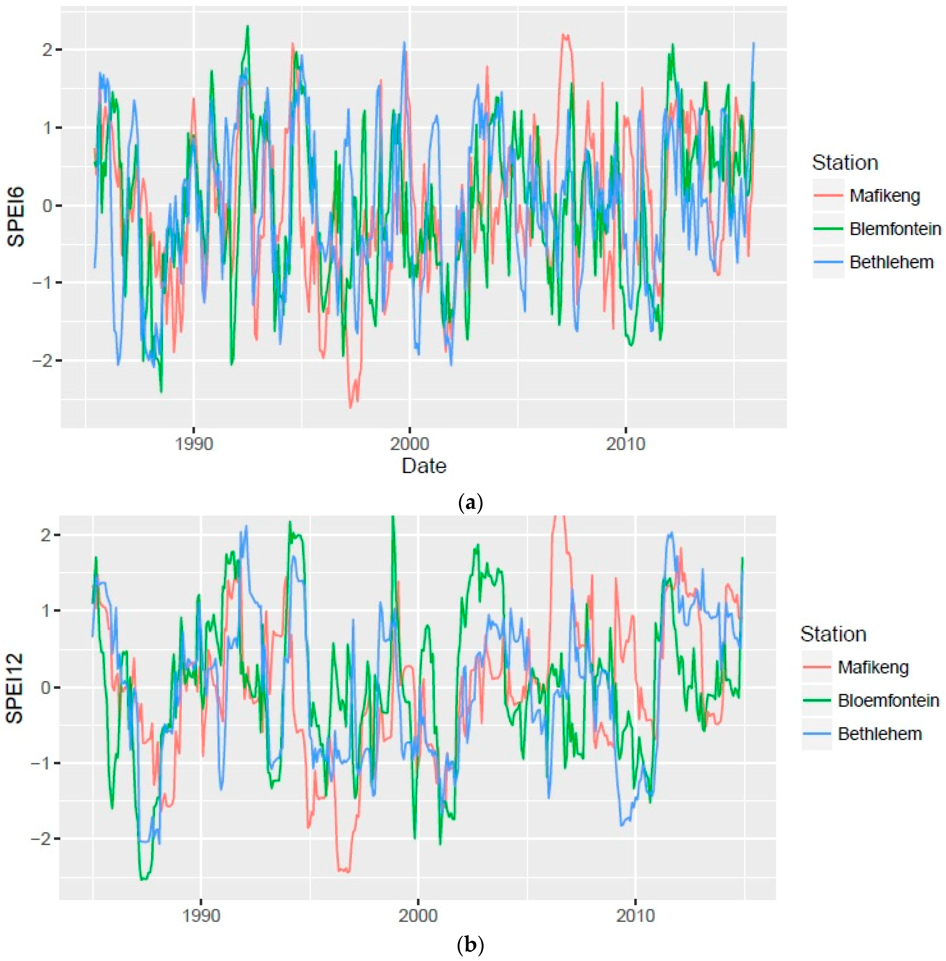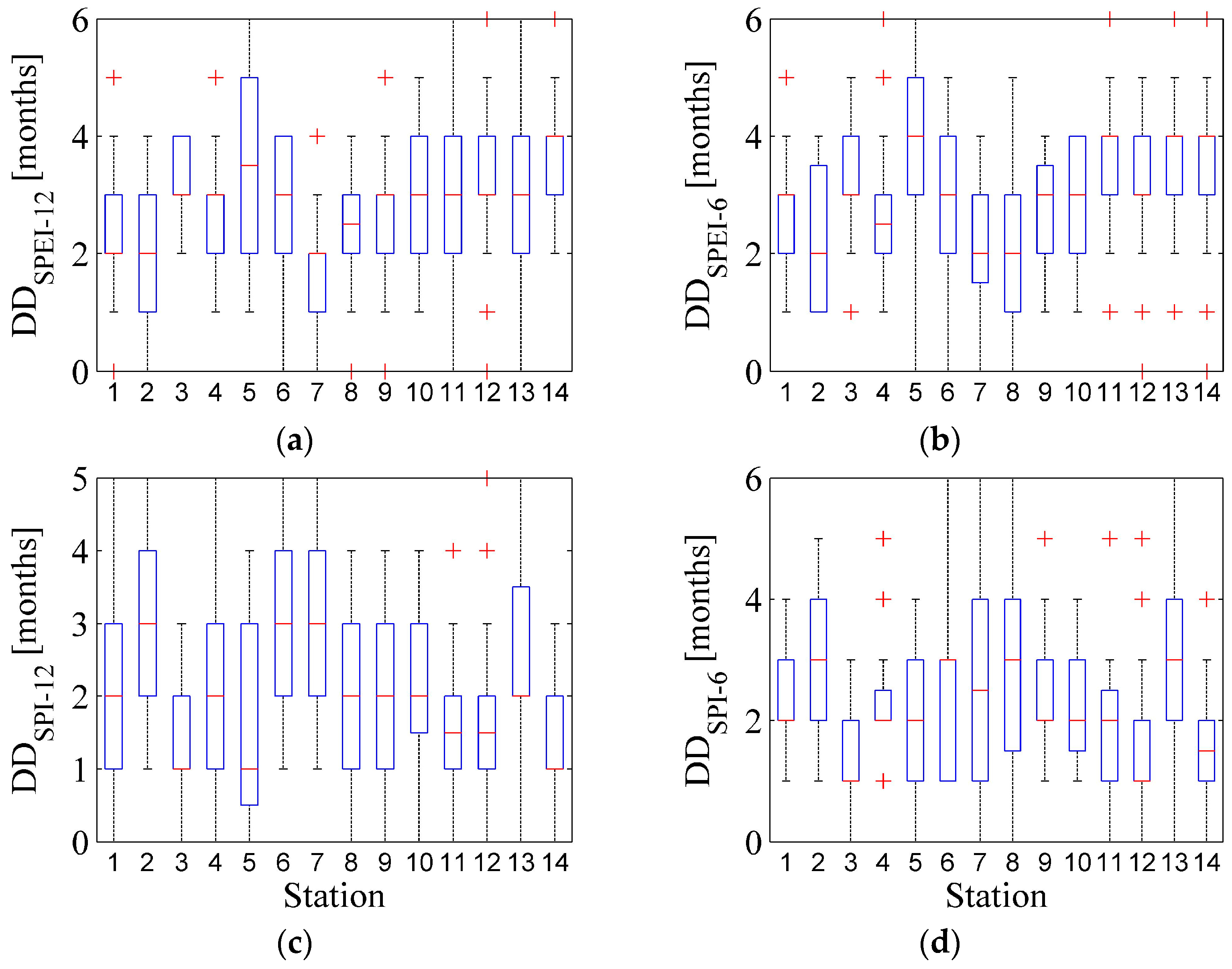[25], SPEI is computed at various temporal scales based on non-exceedance probability of precipitation and potential evapotranspiration differences. The index has the capability to depict the multi-temporal nature of drought. Both SPI and SPEI can be calculated on different timescales, with 1-, 3-, 6-, 12- and 24-months being commonly used [6]. Drought at 1-, 3-, and 6-month timescales is relevant for agricultural impacts, while 12- and 24-month scales are relevant to hydrological and socio-economic impacts, respectively [26].

The SPI and SPEI drought indices have been applied in various studies focusing on drought monitoring as well as prediction of drought class transitions. In particular, a number of studies, including Paulo et al. [27] and Paulo et al. [28] and references therein, have suggested that SPI is more superior, particularly, for drought monitoring purposes. A comparison study of the SPI and SPEI indices at 9- and 12-month time scales reported in Paulo et al. [29] found that SPI and SPEI produced similar results for the same time scales concerning drought occurrence and severity. On the other hand, analysis of SPI and SPEI by Tan et al. [3] suggested that SPEI is instead more applicable than SPI for exploring the spatial-temporal evolution of climate change and drought variation in Ningxia. A multiple timescales study by Törnros and Menzel [30] highlighted the importance of selecting a correct choice of SPEI/SPI timescale when addressing drought conditions related issues under changing conditions. In particular, the authors identified a 6-month SPEI timescale as the most appropriate index, and suggested that a very short timescale would probably fail to detect longer periods of abnormal wet/dry conditions while redundant information is likely to be included if a very long timescale is considered. Studies involving prediction of drought class transitions include among others, Moreira et al. [31], Paulo and Pereira [32], Moreira et al. [33] and references therein.

Application of both SPI and SPEI as drought indicators during monitoring of drought events provides better approach in understanding the response of natural and man-made ecosystem in terms of water supply-demand [34] as well as understanding the evolution of drought in selected areas of interest. This study aims to characterize the nature of droughts over Free State (FS) and North West (NW) Provinces, South Africa based on the SPI and SPEI drought monitoring parameters. Generally, South Africa is classified as a semi-arid and water stressed country. The country’s average annual rainfall is about 450 mm a year, which is below the world’s 860 mm average per year. In particular, rainfall in South Africa exhibits seasonal variability, with most rainfall occurring mainly during summer months (November through March). However, in the southwest region of the country, rainfall occurs in winter months (May through August). South Africa experiences rainfall that varies significantly from west to east. Annual rainfall in the northwest region often remains below 200 mm, whereas much of the eastern Highveld receives between 500 mm and 900 mm (occasionally exceeding 2000 mm) of rainfall per annum. The central part of the country receives about 400 mm of rain per annum, with wide variations occurring closer to the coast. Most regions receiving 400 mm of rainfall play a significant role, e.g., land to the east are suitable for growing crops while land to the west are suitable for livestock grazing as well as crop cultivation on irrigated land. The FS and NW Provinces fall within regions that receive less than 500 mm of rainfall per year, and play an important role towards South African economy. In this regard, the objective of our analysis is focused on investigating historical drought conditions over the two provinces of South Africa, which mainly harbor agricultural production and have the country’s major water reservoirs. Drought characterization over these provinces is valuable in respect of understanding the risks of droughts and determination of the impacts of droughts on agriculture and water resources. A quantitative analysis of Drought Evaluation Indicators (DEIs) such as duration, severity, intensity and frequency (including underlying probability distributions in the DEIs) over southern Africa is, to our knowledge, inconclusive or completely lacking in the literature. Therefore, this study contributes to the theoretical body of knowledge of droughts (through expounding the nature of trends in the DEIs). Results of this work could contribute towards the design of drought preparedness plans in a bid to manage future anticipated drought impacts in South Africa.

2. Study Area

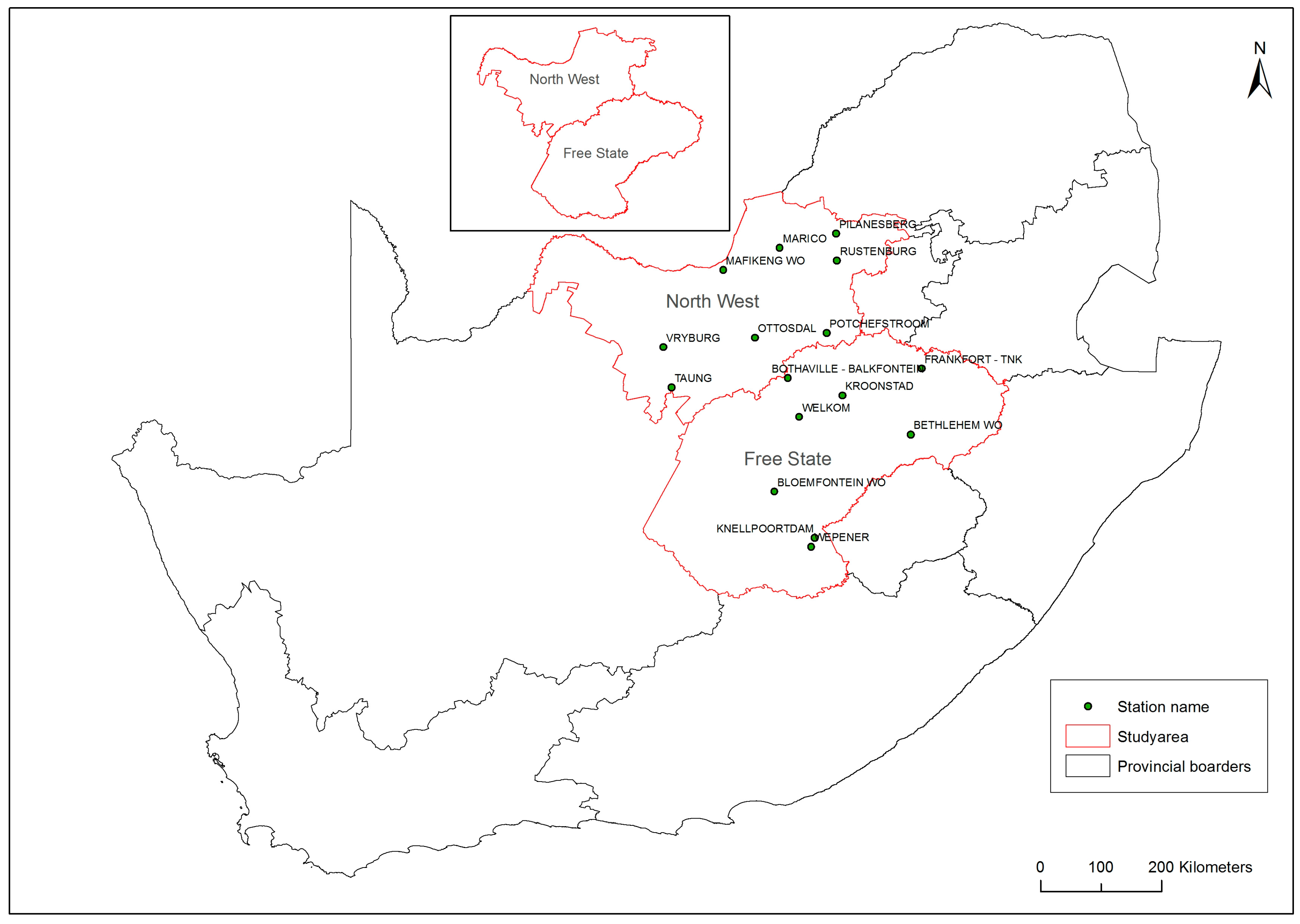
This study focused on two of the nine provinces of South Africa, FS and NW, see Figure 1. Free State is the third largest province in South Africa in terms of land area, with approximately 129,825 km². This represents a 10.6% of the country’s land area [35]. The province is situated between latitudes 26.6° S and 30.7° S and between longitudes 24.3° E and 29.8° E. It borders Lesotho and six other provinces, namely: Northern Cape, North West, Gauteng, Mpumalanga, Eastern Cape and KwaZulu-Natal. The main economic activities contributing significantly towards the gross domestic product of the province are community service (24.7%), agriculture (20.1%), trade (10.7%) and mining (9.6%) [36]. Free State Province contributes significantly to the agricultural economy of the country, e.g., approximately 30% of the national maize production is from the Free State [37]. Agriculture in the province is highly dependent on rainfall, only 10% or less of the arable land is under irrigation. On the one hand, NW Province is situated towards the western part of South Africa and it borders Limpopo Province to the North, Gauteng to the East, FS to the East and South, Northern Cape to the South-West and Botswana to the West and North (see Figure 1). NW Province has a total land area of 116,320 km² and it occupies 9.5% of the total area of South Africa. It is predominantly rural at 65% and 35% urban with agriculture being the main activity. Its land can be characterized as follows: 28% potentially arable, 56.8% grazing, and 14.9% conserved (e.g., for game reserves and housing).

FS and NW Provinces exhibit numerous but significant characteristics that contribute to the country’s economy. For example, in the national context, the NW Province is the highest in cereal and oil seeds production followed by FS. In addition, NW is the highest sheep producer (31.55%) followed by FS, and second largest cattle produce at 17.11% after FS Province [38]. Nevertheless, various constraints, including the lack of or insufficient water, impede farmers from farming effectively. With the recent drought conditions experienced in various parts of South Africa, farmers are battling to keep their animals and crops alive. Most of the farmers in NW and FS rely on rainfall for agriculture activities. Therefore, insufficient rainfall, which ultimately leads to drought, means increased feed costs for the farmers and the few with irrigation schemes will have to pay more costs for irrigation. In recent months, NW and FS Provinces were declared drought disaster areas following the unprecedented poor rainfall and heat waves. The two provinces were selected in this study to investigate the evolution of drought over the past 30 years.

3. Data and Method

3.1. Data Sets

In this study, historical time series of daily precipitation and minimum and maximum temperature from 14 weather stations covering the period 1985–2015, from FS and NW Provinces, South Africa, were analyzed, see for example,

Table 2. List of climate stations used in the drought analysis study. The table summarizes the coordinates of the selected weather stations, including their altitudes, mean annual precipitation (MAP) in mm, mean annual temperature (MAT) in °C and potential evapotranspiration (PET).

Climate Station No.	Station	Latitude	Longitude	Altitude	MAP (mm)	MAT (°C)	PET (mm/year)
0331585 9 (FS)	Bethlehem	−28.2496	28.3343	1689	604	14.3	218.65
0261516B0 (FS)	Bloemfontein	−29.1039	26.2981	1354	466	16.1	187.99
0399894 4 (FS)	Bothaville	−27.4058	26.5044	1267	334	17.9	136.91
0403886A0 (FS)	Frankfort	−27.2672	28.4946	1509	560	15.5	218.81
0365398 8 (FS)	Kroonstad	−27.6665	27.3136	1440	425	17.1	164.09
0508047 0 (NW)	Mafikeng	−25.8037	25.5428	1281	445	19.3	177.86
0546630 3 (NW)	Marico	−25.4718	26.3819	1082	442	19.8	184.27
0360453A0 (NW)	Ottosdal	−26.8145	26.0107	1498	467	17.3	185.20
0548375A4 (NW)	Pilanesberg	−25.2573	27.2238	1085	446	20.0	184.63
0437104A4 (NW)	Potchefstroom	−26.7359	27.0755	1351	450	17.9	183.69
0511399 X (NW)	Rustenburg	−25.6607	27.2322	1150	455	19.3	182.71
0360453A0 (NW)	Taung	−27.5452	24.7687	1115	353	19.5	150.16
0432237 3 (NW)	Vryburg	−26.9547	24.6527	1245	400	18.3	170.43
0364300 1 (FS)	Welkom	−27.9947	26.6660	1344	374	18.1	153.12

for the summary of the selected stations. Based on Table 2 the mean annual precipitation varies across different weather stations. For instance, Bethlehem weather station in FS Province has the highest MAP of about 60 mm, whereas Bothaville, also in FS, has the lowest MAP (~33 mm). Variations can be attributed to topography as well as weather or climate conditions. Weather stations often suffer from missing data, which makes it difficult to have a continuous time series of the selected period of study. Gap filling process (where climatological median values) was used in cases where there were gaps. This simple gap filling process was considered because the stations with gaps (four stations) had less than 1% of gaps. Monthly precipitation totals were calculated from daily precipitation datasets. The SPI and SPEI analysis method requires a minimum data period between 20 and 30 years, hence the selected period was chosen in order to provide at least 30 years of data records.

3.2. Methodology

In the present study, droughts have been characterized based on two commonly used drought indices, i.e., SPI and SPEI. The advantages of using SPI and SPEI are premised on the principle of parsimony and their ability to quantify the magnitude, duration, and extent of droughts independently of the local climatic conditions. The SPI drought index is mostly recommended by the World Meteorological Organization (WMO) as a standard drought index [6,39]. Its computation requires only precipitation as an input and has capability to monitor both dry (represented by negative values) and wet conditions (represented by positive values) [40]. In calculating the indices, a minimum of 20 years of data is often required, although the usage of more data sets (e.g., 50–60 years or more) is ideal [41]. The SPI computation involves fitting a gamma distribution to a precipitation time series, for more information on computation of SPI values the reader is referred to McKee et al. [24], McKee et al. [42], Edwards and McKee [43] and references therein.

Computation of SPEI requires a time series of total monthly precipitation (P) data as well as monthly potential evapotranspiration (PET). The monthly PET was calculated based on the approach presented by [44] that only relies on monthly mean temperature (T) and latitude (L), to calculate the monthly average day length. Full details of computing SPEI can be found in [25]. Due to similarities in the calculation principles of SPEI and SPI, see studies by McKee et al. [24], Kumar et al. [45] and Banimahd et al. [46] and references therein, both indices have same classification criteria, as summarized in

Table 3. Standardized Precipitation Index classification [42].

Level	SPI Value	Class	Cumulative Probability	Probability of Event (%)
1	−1.00 < SPI ≤ 0	Mild drought	0.50000	68.2
2	−1.50 < SPI ≤ −1.00	Moderate drought	0.15866	9.2
3	−2.00 < SPI ≤ −1.50	Severe drought	0.06681	4.4
4	SPI ≤ −2.00	Extreme drought	0.02275	2.3

. The more the negative the SPI/SPEI value, the more severe the drought.

In order to characterize the historical droughts in the present study, 6- and 12-month SPI and SPEI indices were calculated from pre-processed monthly precipitation and minimum and maximum temperature using SPI R package. The resulting SPI/SPEI time series were then sub-set in order to use only data for October to April months. The selected months were considered because they represent the season when drought conditions are manifest in South Africa. The resulting time series was analyzed as summarized in the following algorithm:

Step I.

For each station, a Drought Time series (hereafter DTs) was derived based on the selecting only dry months

Step II.

The DTs derived in Step I was used to compute the DEIs, i.e., Drought Duration (DD), Drought Severity (DS), Drought Intensity (DI) and Drought Frequency (DF). As reported in Tan et al. [3], the duration (m) of a drought event is equivalent to the number of months between its onset and end month. On the other hand, the severity (DS_e) and intensity (DI_e) may be calculated using the following equations described in Tan et al. [3]:

$$D{S}_e={\left|{\displaystyle \sum }_{j=1}^{m}Inde{x}_j\right|}_e$$

(1)

$$D{I}_e=\frac{S_e}{m}$$

(2)

In Equation (1), e corresponds to a drought event; j to a month; Index_j is the SPI/SPEI value in month j; an m, S_e and DI_e are the duration, severity and intensity of a drought event e, respectively. The drought frequency was calculated based on Equation (3):

$$D{F}_s=\frac{n_s}{N_s}\times 100\%$$

(3)

where n_s equals the number of drought events, N_s is the total number of years for the study period and s is a station.

Step III.

Furthermore, the DTs and DEIs were used to compute the trends. In particular, two methods were used to compute the trends of DTs and DEIs. The first method was based on pre-whitening (hereinafter referred to as the “z” method) linear trend analysis procedure proposed by Zhang et al. [47]. This method assumes that both DTs and DEIs series are composed of a long-term trend component and a white noise residual component, thus enabling incorporation of statistical regression model with serially correlated residuals described by Equation (4).

$$Y_t=\mu +T_t+v_t$$

(4)

where Y_t is a climate variable at time t, µ is the constant term, T_t is the trend and v_t is the noise at time t. Equation (4) can be simplified by assuming a linear trend, that is,

$$Y_t={\beta }_t$$

(5)

where β represents the slope of the linear region between the climate variable and time. On the other hand, the noise may be expressed as per Equation (6),

$$v_t={\displaystyle \sum }_{r=1}^p{\varnothing }_r{v}_{t-r}+{\epsilon }_t$$

(6)

where ${\varnothing }_r$ the parameters of the autoregressive are process, p is the order of the auto-regression and $\left\{{\epsilon }_t\right\}$ is white noise. Thus, Equation (4) can be re-written as

$$Y_t=\mu +{\beta }_t+{\varnothing }_r{Y}_{t-1}+{\epsilon }_t$$

(7)

where by lag-one autocorrelation, AR(1) was utilized. The second method used was based on trend free pre-whitened trend analysis (hereinafter referred to as the “y” method) described in Yue et al. [48]. This method assumes that a hydrological time series can be represented by a linear trend given by

$$T_t=bt$$

(8)

and an AR(1) component with noise. In Equation (10), b is represents the slope each combined series and it is estimated using Theil-Sen Approach (TSA) proposed by Theil [49], Theil [50] Theil [51] and [52]. Assuming that the slope is not zero, then linearity is assumed whereby the DTs and DEIs are detrended using

$$X_t^{\text{'}}=X_t-T_t=X_t-bt$$

(9)

The trend-free pre-whitening procedure is achieved by detrending the series $X_t^{\text{'}}$ using time lag serial correlation coefficient $r_1$ and then removing the AR(1) from the series, as per Equation (10),

$$Y_t^{\text{'}}=X_t^{\text{'}}-r_1{X}_{t-1}^{\text{'}}$$

(10)

The residual series after applying the trend-free pre-whitening procedure results in an independent series. The identified trend T_t and the residual $Y_t^{\text{'}}$ are blended by

$$Y_t=Y_t^{\text{'}}+T_t$$

(11)

The MK test was then applied to the blended series $Y_t$ to assess the significance of the DTs and DEIs time series. The two methods using in this study are capable of handling the impact of serial autocorrelation on trend detection of DTs and DEIs.

4. Results

4.1. Drought Characterization

Figure 2a,b depict SPEI 6 and 12 time series, respectively, derived from Mafikeng, Bloemfontein and Bethlehem weather stations. Both drought indices provide similar results related to drought variability and trends across the selected study area. In particular, the results indicate that SPEI time series at 6- and 12-month time scales exhibit both seasonal and inter-annual drought variability. There are few cases where the SPEI values show inter-seasonal drought variation, particularly the SPEI-6 time scale. In order to better understand the behavior of the SPI and SPEI indices across FS and NW Provinces, trends of the DTs were performed for the 14 selected weather stations for the period spanning 1985–2015. The results from the trend analysis are presented in Figure 3 ((a) SPEI and (b) SPI) and

Table 4. Results of the trend test applied to DTS and the corresponding significance.

Station	SPI				SPEI
	6y	6z	12y	12z	6y	6z	12y	12z
	τ (p-value)	τ (p-value)	τ (p-value)	τ (p-value)	τ (p-value)	τ (p-value)	τ (p-value)	τ (p-value)
Bethlehem	−0.004 (0.15)	0.003 (0.15)	−0.003 (0.29)	−0.003 (0.29)	−0.006 (0.02)	−0.005 (0.02)	−0.010 (0.01)	−0.007 (0.01)
Bloemfontein	−0.003 (0.06)	−0.003 (0.15)	−0.001 (0.44)	−0.001 (0.44)	0.002 (0.44)	0.001 (0.44)	−0.001 (0.86)	0.000 (0.87)
Bothaville	0.004 (0.06)	−0.003 (0.05)	0.004 (0.36)	0.006 (0.36)	0.002 (0.51)	0.003 (0.49)	0.001 (0.64)	0.003 (0.62)
Frankfort	−0.001 (0.74)	0.004 (0.06)	−0.002 (0.37)	−0.001 (0.37)	0.000 (1.00)	0.000 (1.00)	0.003 (0.28)	0.003 (0.28)
Kroonstad	0.004 (0.02)	0.000 (0.74)	0.004 (0.02)	0.004 (0.04)	−0.001 (0.53)	−0.001 (0.53)	−0.002 (0.59)	−0.003 (0.58)
Mafikeng	−0.003 (0.18)	0.004 (0.00)	−0.001 (0.47)	0.000 (0.47)	0.000 (0.91)	0.000 (0.86)	0.003 (0.33)	0.003 (0.33)
Marico	0.000 (0.95)	−0.002 (0.18)	−0.001 (0.85)	0.000 (0.85)	0.003 (0.06)	0.003 (0.06)	0.005 (0.01)	0.006 (0.01)
Ottosdal	0.004 (0.05)	−0.001 (0.95)	0.003 (0.56)	0.002 (0.57)	−0.001 (0.80)	0.000 (0.79)	0.001 (0.69)	0.001 (0.69)
Pilanesberg	0.001 (0.77)	0.004 (0.05)	−0.002 (0.50)	0.001 (0.51)	0.002 (0.31)	0.002 (0.13)	0.003 (0.01)	0.004 (0.01)
Potchefstroom	0.000 (0.77)	0.001 (0.78)	−0.001 (0.73)	0.000 (0.73)	−0.002 (0.24)	−0.002 (0.24)	−0.006 (0.04)	−0.003 (0.03)
Rustenburg	0.004 (0.01)	0.000 (0.76)	0.005 (0.04)	0.006 (0.04)	0.002 (0.16)	0.002 (0.15)	0.001 (0.76)	0.001 (0.77)
Taung	0.002 (0.47)	0.005 (0.01)	0.004 (0.17)	0.004 (0.16)	0.002 (0.31)	0.003 (0.31)	−0.001 (0.78)	0.000 (0.77)
Vryburg	−0.001 (0.54)	0.002 (0.46)	−0.001 (0.52)	−0.001 (0.52)	−0.005 (0.03)	−0.004 (0.03)	−0.005 (0.18)	−0.005 (0.18)
Welkom	0.004 (0.10)	−0.001 (0.52)	0.007 (0.02)	0.007 (0.01)	0.004 (0.23)	0.004 (0.22)	−0.002 (0.65)	−0.001 (0.65)

. As depicted in Figure 3, positive and negative trends exist across all the stations. Furthermore, only few stations exhibit statistically significant trends. The trends calculated using the two methods (“y” and “z”), as given in Figure 3a,b, show larger negative trends over Bethlehem, Bloemfontein, and Vryburg weather stations, while larger positive trends are observed at Bothaville, Ottosdal, Pilanesberg, Rustenburg, Taung and Welkom weather stations. Additionally, 64% and 57% of the stations exhibit SPI-6 and SPEI-6 positive trends, respectively. On the other hand, 43% and 50% of the stations exhibit negative SPI-12 and SPEI-12 positive trends, respectively. The rest of the weather stations exhibit both positive and negative trends, with some of the trend results contrasting between the two analysis methods used. Overall, it can be concluded that both trend analysis methods yield similar results, albeit with subtle differences that could be attributed to the differences in the length of the DTs considered in the present study.

Table 4 summarizes trend analysis and the corresponding significance test results applied to the DTs using the “y” and “z” methods. In this study, trends in DTs are considered significant if the estimated p-value falls below a critical value (e.g., α < 0.05), indicating 95% confidence [49]. In Table 4, the τ values in each column indicate the trend while p-values in brackets of τ designate the significance of trends. The results presented in Table 4 indicate that both the drought indices at the considered time scales exhibit both positive and negative trends across all the stations illustrating that the trends exhibit spatial temporal variability. There is an increasing trend in both DTs although most of the observed trends are insignificant.

Generally, the observed trends in DTs demonstrate that the impact of droughts could be significantly different across the two provinces. In particular, it can be noticed that about 60% of the weather stations exhibit decreasing trends and that most of these stations are situated in FS Province. This suggests that the FS Province experienced persistent drought conditions during the analyzed period as compared to NW. As a result, key sectors such as agriculture and water resources are likely to be affected negatively. These conditions are a thread to the food security given that the province is considered to be the food basket of South Africa. The increasing droughts will decrease the volumes in water reservoirs and streams, which are largely located in (and also transect across) the provinces under the present study.

The DEIs such as DS, DD, DI, and DF are parameters that can be used to objectively quantify the impacts of droughts in an area. Given in Figure 4, Figure 5, Figure 6, Figure 7, Figure 8 and Figure 9 are the DS, DD, DI and DF calculated at 14 automatic weather stations across FS and NW Provinces. As shown in Figure 4, the DS derived from SPEI-12 (Figure 4a) is consistent with that calculated from SPEI-6 (Figure 4b). On the other hand, DS calculated from SPI (Figure 4c,d) exhibit inherent differences across the stations and within the different timescales. These differences could be attributed to the inherent outliers. Overall, the DS varies between 1 and 4 across the two provinces.

Figure 5 and Figure 6 depict the median and extremes of intensity of droughts, respectively, across the study area. While differences in the DI derived from SPEI-12 and SPEI-6 exist (and also the SPI-12/-6), the overall range in the DI is between 0.5 and 2.0 (the SPI has the largest range of 3.3) (see Figure 5). Furthermore, 50% of the stations exhibit a maximum DI greater than 2.0 while most stations have a minimum median value less than 0.5. During 1985–2015, most stations (71%) had average DI calculated from SPI-6 greater than those calculated from SPI-12. On the other hand, only 36% of the stations yielded average SPEI-6 DI greater than the average DI derived from SPEI-12. These proportions are reflected similarly in the standard deviations. These contrasting results point to a research question of developing a methodology to determine the most appropriate index that could be used to calculate the DI in southern Africa. This is the subject of the current on-going investigation.

In Figure 7 and Figure 8, the number of months exhibiting drought conditions across FS and NW Provinces are provided. As illustrated in Figure 6, the DD calculated from SPEI-12 are comparable to the DD derived from SPEI-6, albeit with subtle outliers. Additionally, the DD derived from SPI-12 and SPI-12 are similarly comparable. Furthermore, in 71% of the stations, the DDs derived from SPEI-6 and SPI-6 are greater than the DDs derived from SPEI-12 and SPI-12. This similarity suggests that calculating the DD is not dependent on whether one is using the SPI or SPEI index. In the period between 1985 and 2015 drought months, the maximum number of drought months varies between three and six months, while minimum number of drought months range between 0 and two across the study region. As depicted in Figure 8, between 1985 and 2015, the average DD across the study area is approximately two months. In particular, up to 48% of the stations record average DD value of three months while the majority of the stations exhibit extreme DD values of up to six months. These values suggest that the study area experiences prolonged droughts of category one (short-term droughts) and two (medium-term droughts). As a result, the observed rainfall deficiencies of sufficient magnitude over prolonged durations and extended areas (as demonstrated by the DD values) could lead to the subsequent reductions in the streamflow. All of these will consequently interfere with the normal agricultural and economic activities of the study region. These conditions may lead to decrease in agriculture production, subsequently impacting on the livelihoods of the populace.

As shown in Figure 9 and Figure 10, spatial differences of the DFs across the study area exist. In this regard, 71% of the stations exhibit larger DF values derived from SPI-6/SPEI-6 compared to SPI-12/SPEI-12. This suggests that DF could be a robust drought evaluation indicator (similar to DD) independent of the type of drought index under consideration. As illustrated in Figure 8, the overall median frequency of drought events across the entire study area lies between 5% and 12%, centering at approximately 7%, while the extremal DF value is up to approximately 19.4% (see Figure 9). Furthermore, most stations exhibit extreme maximum (or minimum) DF values above 10% (or 3%). These results suggest that farmers in the NW and FS Provinces have been experiencing extreme weather/climate conditions, which could impact on their productivity.

Table 5. Trends in drought severity of SPI/SPEI-6/12 across the selected weather stations.

Station	SPI		SPEI
	6-month	12-month	6-month	12-month
	τ (p-value)	τ (p-value)	τ (p-value)	τ (p-value)
Bethlehem	0.010 (0.90)	0.039 (0.45)	−0.085 (0.14)	−0.010 (0.87)
Bloemfontein	0.023 (0.67)	−0.007 (0.83)	−0.021 (0.54)	−0.034 (0.61)
Bothaville	0.038 (0.24)	0.005 (1.00)	0.000 (0.97)	0.003 (0.89)
Frankfort	0.063 (0.15)	0.115 (0.00)	−0.056 (0.24)	−0.009 (0.78)
Kroonstad	0.088 (0.01)	0.059 (0.10)	−0.137 (0.02)	−0.178 (0.02)
Mafikeng	0.014 (0.72)	−0.005 (0.91)	0.019 (0.67)	−0.009 (0.75)
Marico	0.040 (0.41)	0.109 (0.18)	0.000 (0.97)	−0.019 (0.56)
Ottosdal	0.030 (0.34)	0.019 (0.25)	0.007 (0.80)	0.001 (1.00)
Pilanesberg	0.047 (0.09)	0.059 (0.21)	−0.016 (0.50)	0.005 (087)
Potchefstroom	0.039 (0.25)	0.056 (0.07)	−0.028 (0.59)	−0.040 (0.32)
Rustenburg	0.071 (0.07)	0.053 (0.04)	−0.049 (0.12)	−0.021 (0.52)
Taung	0.067 (0.10)	0.133 (0.04)	−0.074 (0.15)	−0.039 (0.69)
Vryburg	0.027 (0.69)	0.050 (0.25)	−0.010 (0.75)	0.049 (0.39)
Welkom	0.079 (0.00)	0.068 (0.02)	−0.057 (0.18)	−0.098 (0.24)

gives results of pre-whitening trend analysis of the DS time series derived from the SPI and SPEI indices. In particular, 100% and 86% of the stations exhibit positive DS trends derived from SPI-6 and SPI-12, respectively. For SPI-6, only Kroonstad and Welkom stations have statistically significant positive trends while Frankfort, Rustenburg, Taung and Welkom exhibit statistically positive DS trends derived from SPI-12. On the other hand, 79% of the stations exhibit negative DS trends (only Kroonstad has statistically significant trend) derived from both SPEI-6 and SPEI-12. These results suggest that the DS estimated from SPI and SPEI time series may not robustly characterize the trends of droughts across the study area. This finding could be attributed to the inherent differences in calculating the DTs, limitations of temporal resolution as well as the minimal number of drought seasons under consideration.

Table 6. Trends in drought intensity of SPI-6 and SPEI-12 across the selected weather stations.

Station	SPI		SPEI
	6-month	12-month	6-month	12-month
	τ (p-value)	τ (p-value)	τ (p-value)	τ (p-value)
Bethlehem	−0.014 (0.44)	τ (p-value)	−0.032 (0.03)	-0.020 (0.41)
Bloemfontein	−0.005 (0.50)	−0.007 (0.66)	−0.002 (0.59)	−0.041 (0.01)
Bothaville	0.000 (1.00)	−0.007 (0.38)	0.008 (0.07)	0.009 (0.03)
Frankfort	0.004 (0.68)	−0.039 (0.63)	−0.004 (0.77)	0.005 (0.59)
Kroonstad	0.044 (0.02)	0.015 (0.46)	−0.005 (0.59)	0.003 (0.72)
Mafikeng	0.002 (0.80)	0.022 (0.40)	0.002 (0.92)	−0.001 (1.00)
Marico	0.008 (0.54)	−0.001 (1.00)	0.000 (0.95)	0.000 (0.98)
Ottosdal	0.009 (0.32)	0.022 (0.10)	−0.016 (0.16)	−0.020 (0.05)
Pilanesberg	0.018 (0.04)	−0.005 (0.76)	−0.001 (0.87)	0.001 (0.86)
Potchefstroom	0.022 (0.10)	0.022 (0.07)	−0.010 (0.38)	−0.005 (0.35)
Rustenburg	0.022 (0.13)	0.008 (0.33)	−0.006 (0.41)	0.000 (0.95)
Taung	0.012 (0.46)	0.030 (0.40)	0.008 (0.34)	0.015 (0.23)
Vryburg	0.018 (0.13)	0.047 (0.04)	−0.027 (0.21)	−0.003 (0.91)
Welkom	−0.006 (0.65)	0.012 (0.24)	0.009 (0.40)	0.000 (0.93)

summarizes trend results for DI time series across the considered weather stations. Based on the SPI-6 and SPI-12, we observe increased DI trends particularly in FS Province. In this regard, 79% and 57% of the stations exhibit negative DI trends calculated from SPI-6 and SPI-12 time series. With regard to DI trends calculated from SPEI-6 and SPEI-12 times series, positive trends occur at 36% and 57%, respectively, of the stations considered in the present study. Only stations in FS Province exhibit trends that are statistically significant. Overall, inherent differences in the sign of the trends calculated from DI values derived from SPI/SPEI across the stations exist. These results suggest that the underlying trends in the DI values calculated from the present DTs cannot be used to appropriately characterize the droughts in the study area.

The trends in the frequency of droughts based on SPI and SPEI DTs are depicted in

Table 7. Trends in drought frequency of SPI/SPEI-6/12 across the selected weather stations.

Station	SPI		SPEI
	6-month	12-month	6-month	12-month
	τ (p-value)	τ (p-value)	τ (p-value)	τ (p-value)
Bethlehem	0.136 (0.11)	0.269 (0.08)	0.000 (0.45)	0.027 (0.65)
Bloemfontein	0.066 (0.57)	0.116 (0.34)	0.000 (0.82)	0.000 (0.80)
Bothaville	0.248 (0.01)	0.215 (0.02)	−0.029 (0.28)	−0.050 (0.35)
Frankfort	0.157 (0.09)	0.322 (0.01)	−0.120 (0.34)	0.000 (0.82)
Kroonstad	0.461 (0.00)	0.358 (0.00)	−0.419 (0.01)	−0.488 (0.03)
Mafikeng	0.000 (0.97)	0.094 (0.41)	0.000 (0.89)	0.053 (0.73)
Marico	0.021 (0.64)	0.050 (0.59)	−0.018 (0.68)	0.013 (0.58)
Ottosdal	0.048 (0.82)	0.070 (0.33)	0.000 (1.00)	0.000 (0.61)
Pilanesberg	0.187 (0.16)	0.000 (0.06)	−0.059 (0.42)	0.000 (0.97)
Potchefstroom	0.066 (0.53)	0.161 (0.11)	0.000 (1.00)	0.044 (0.59)
Rustenburg	0.234 (0.05)	0.322 (0.00)	−0.230 (0.05)	−0.051 (0.59)
Taung	0.348 (0.02)	0.532 (0.01)	−0.269 (0.08)	−0.390 (0.12)
Vryburg	0.083 (0.59)	0.147 (0.15)	−0.248 (0.24)	0.000 (0.99)
Welkom	0.331 (0.00)	0.333 (0.00)	−0.197 (0.04)	−0.204 (0.17)

. Results show that the trends in the frequency of droughts derived from the SPI-6 and SPI-12 DTs across all the considered weather stations exhibit increasing trends with approximately 30% (DTs of the SPI-6) and approximately 50% (DTs of the SPI-12) cases showing trends that are statistically significant. On the contrary, the frequency of droughts derived from SPEI DTs seems to demonstrate largely negative trends in 64% (SPEI-6) and 36% (SPEI-12) of the stations.

4.2. Drought Categories

In this study, the SPI and SPEI drought indicators were used to establish drought duration, in terms of the drought categories defined in Table 3, within the selected study regions. For this purpose, the time scale was divided into three decades, i.e., 1985–1994, 1995–2004 and 2005–2015. The results for this analysis are depicted in Figure 11 for SPI/SPEI-6 and Figure 12 and for SPI/SPEI-12 drought indices. In Figure 11, (a) depict mild drought events, (b) moderate drought occurrences, (c) severe drought events, and (d) events of extreme droughts within the two selected provinces. Based on SPI-6 drought indicators, there is a significant increase in mild drought events in the FS Province, from shorter time steps (first decade) to longer time steps (third decade). In the NW Province, mild droughts remained the same between the first and third decades and slightly decreased between 1995 and 2004. On contrary, SPEI-6 depicts an increase in mild drought occurrences from the shorter-time steps to the medium-time steps and a sudden decrease thereafter during the third decade. In addition, based on SPEI-6, mild drought occurrences in NW Province remained relatively at the same level at shorter-time steps and longer-time steps but increased at medium-time steps.

Occurrences of moderate drought are undetected by the SPI-6 drought index. However, based on SPEI-6, there is an increase of moderate drought during the first decade, but it stayed relatively stable during the second and third decades in both FS and NW. Furthermore, based on both SPI- and SPEI-6, severe droughts demonstrated persistence in FS during the first and second decades. On the other hand, SPI-6 detected an increase in severe droughts during the first decade, becoming negligible during the second decade and significantly increasing during the third decade. Based on SPEI-6, severe droughts have increased during the first and second decades but decreased during the third decade. Extreme droughts are only detected by SPI-6 in NW during the third decade and SPEI-6 in FS during the second decade.

Figure 12 depicts drought duration events based on SPI- and SPEI-12 drought indicators across the selected stations. Similarly to Figure 11, in Figure 12, (a) depict mild drought events, (b) moderate drought occurrences, (c) severe drought events, and (d) events of extreme droughts within the two selected provinces. Based on SPI-12, mild droughts increased significantly from 1985 to 2015 in FS. Similar results are observed for SPEI-12, although drought occurrences seem to have slightly decreased during the third decade (e.g., 2005–2015). Mild drought occurrences seem to have remained relatively high during the first and third decades, while decreasing during the second decade in the NW Province. On the contrary, SPEI-12 indicator depicts significant evolving mild drought occurrences during the first and second decades, which decrease thereafter during the third decade.

Results in Figure 12b depict a decrease in moderate drought occurrences in FS Province for SPI-12. Occurrences of moderate droughts in NW remained relatively on the same level during the first and second decades, with a significant increase during the third decade (see SPI-6). Results for SPEI-12 depict similar trends in both provinces. In particular, moderate drought occurrences evolved during the first and second decades with a decrease during the third decade. Based on SPI-12, FS experienced significant severe droughts during the third decade. On contrary, significant severe drought occurrences in both provinces were detected in SPEI-12. For instance, during the middle decade, the events seem to decrease at longer time steps (2005–2015), relatively to the same duration level (~0.15) observed for SPI-6 in FS. Extreme drought occurrences are observed in NW Province during the third decade (see, SPI-12). In addition, based on SPEI-12, both FS and NW Provinces have experienced extreme drought events at longer time steps (2005–2015).

In general, the analysis of drought occurrences indicates that different categories of droughts occur at different time steps. Drought occurrences in the selected regions tend to evolve from a shorter-time scale, increasing with increased time scale. In some cases, drought occurrences evolved from shorter-time steps to medium-time steps and decreases thereafter at longer-time steps. Overall, FS Province seems to have experienced more drought occurrences during the analyzed period. The observed drought categories have significant consequences to various sectors, ranging from agriculture to water.

5. Discussion

South Africa has suffered one of the worst droughts of the century. It has been linked to climate change and the recounting El Niño phenomenon, which warms surface waters in the eastern tropical Pacific Ocean. The ensuing lack of rain and soaring temperatures have decimated the agricultural sector and forced urban water restrictions as the water reservoirs continue to be below 50% capacity. Having been inundated by these conditions, the present study characterized the nature of historical drought conditions across two South African provinces, often considered to be central for food and water security of the country. In particular, the study considered a drought characterization metric consisting of the drought duration, drought severity, intensity and frequency as drought monitoring indicators. While illustrating that the characteristics of droughts exhibit subtle trends, the duration, severity, intensity of droughts in the two provinces exhibit noticeable spatial-temporal differences. These findings have critical implications to both the agricultural sector and water resources in South Africa, which is already categorized as a water stressed country.

5.1. Implications to the Agricultural Sector

Droughts often manifest in terms of lack of rainfall and high temperatures. These two climate parameters are the key drivers of the hydrological cycle. A disturbance in any one component or process of the hydrological cycle has impacts on the agricultural cycle. To this end, the immediate consequence of drought is a fall in crop production, due to inadequate and poorly distributed rainfall. Additionally, livestock production is impacted due to low rainfall, which causes poor pasture growth and may also lead to a decline in fodder supplies from crop residues. It is therefore important to understand the characteristics of historical droughts in order to quantitatively determine their impacts to the Agricultural production in the two provinces. This information is especially important, as it could enable stakeholders to develop robust drought monitoring and forecasting tools in support of preparedness for future droughts under changing climate. In this regard, characterizing droughts in the two provinces would enable farmers to make informative decisions related to weather/climate impacts relevant to them.

5.2. Implications to Water Resources

South African water reservoirs have depicted continuous decline over a period of time in corroboration with decreases in the amount and irregularity in the amount of rainfall received throughout the country (in general) and the two provinces (in particular). The status quo of the water reservoirs is expected to be maintained because of the linkage between climate change and variability and the precipitation, run off, evapotranspiration, soil moisture and stream flow. The underlying processes influencing the dynamics of these linkages are complex and remain a hot subject in earth–atmosphere interactions research. Through drought characterization of drought metrics derived from SPI-12 and SPEI-12 work reported in this paper, it is hoped that the hydrological drought monitoring and forecasting efforts would be the backbone of robust water resources planning across the two provinces. The planning is no doubt significant for reducing the economic, social and environmental negative impacts of changes in weather and climate.

6. Conclusions

In order to determine potential risk of droughts occurring in future, it is vital to thoroughly analyze the historical drought events. The impact of drought depends on severity, duration and spatial extent of the rainfall deficit. In this study, we have used SPI and SPEI indices to study the characteristics of drought in FS and NW Provinces. Following a continued deficit of rain in the country, the government of South Africa has declared FS and NW together with three other provinces drought disaster areas, consequently threatening food security in the country. The current contribution aimed to quantify the severity, duration and the spatial extent of drought over the two considered provinces, based on the drought monitoring indices derived from SPI and SPEI. The goal of the present study was to understand the drought characteristics (e.g., evolution, frequency, intensity and severity) rather than comparing the SPI and SPEI derived indices. Generally, the evolution of drought is noticeably observed in the two provinces, although there are very few cases where the observed negative trends result in statistically significant trends. Analysis of drought evaluation indicators (DEIs), calculated from SPEI suggest that drought severity and frequency was more pronounced in FS while the intensity of the drought was more in NW Province during 1985–2015. In addition, based on SPEI calculations, moderate drought occurrences increased during 1985–1994 and 1995–2004 periods and decreased thereafter (2005–2015) in both considered provinces. SPEI produced similar results for mild drought occurrences during the same time scales. Occurrences of severe droughts indicate decreasing signs from 1995–2004 towards 2005–2015 period.

References

1. Wilhite, D.A.; Svoboda, M.D.; Hayes, M.J. Understanding the complex impacts of drought: A key to enhancing drought mitigation and preparedness. Water Resour. Manag. 2007, 21, 763–774. [Google Scholar] [CrossRef]
2. Vicente-Serrano, S.M.; Begueria, S.; Eklundh, L.; Gimeno, G.; Weston, D.; Kenawy, A.E.; Lopez-Moreno, J.I.; Nieto, R.; Ayenew, T.; Konte, D.; et al. Challenges for drought mitigation in Africa: The potential use of geospatial data and drought information systems. App. Geogr. 2012, 34, 471–486. [Google Scholar] [CrossRef] [Green Version]
3. Tan, C.; Yang, J.; Li, M. Temporal-spatial variation of drought indicated by SPI and SPEI in Ningxia Hui Autonomous region, China. Atmosphere 2015, 6, 1399–1421. [Google Scholar] [CrossRef]
4. Zhang, L.X.; Zhou, T.J. Drought over East Asia: A review. J. Clim. 2015, 28, 3375–3399. [Google Scholar] [CrossRef]
5. Wang, L.; Chen, W.; Zhou, W.; Huang, G. Drought in Southwest China: A review. Atmos. Ocean. Sci. Lett. 2015, 8, 339–344. [Google Scholar]
6. Chen, T.; van der Werf, G.R.; de Jeu, R.A.M.; Wang, G.; Dolman, A.J. A global analysis of the impact of drought on net primary productivity. Hydrol. Earth Syst. Sci. 2013, 17, 3885–3894. [Google Scholar] [CrossRef]
7. Dracup, J.A.; Lee, K.S.; Paulson, E.D. On the definition of droughts. Water Resour. Res. 1980, 16, 297–302. [Google Scholar] [CrossRef]
8. Wilhite, D.A.; Glantz, M.H. Understanding the drought phenomenon: The role of definitions. Water Int. 1985, 10, 111–120. [Google Scholar] [CrossRef]
9. Wilhite, D.A. Drought assessment, management, and planning: theory and case studies. In Natural Resource Management and Policy Series; Dinar, A., Zilberman, D., Eds.; Kluwer Academic Publishers: Dordrecht, The Netherlands, 1993. [Google Scholar]
10. Tate, E.L.; Gustard, A. Drought definition: A hydrological perspective. In Drought and Drought Mitigation in Europe; Advances in Natural and Technological Hazards Research Volume 14; Springer Science and Business Media: Dordrecht, The Netherlands, 2000; pp. 23–48. [Google Scholar]
11. Pereira, L.S.; Cordery, I.; Iacovides, I. Coping with water scarcity. In Addressing the Challenges; Springer Science and Business Media: Dordrecht, The Netherlands, 2009; p. 382. [Google Scholar]
12. Halwatura, D.; Lechner, A.M.; Arnold, S. Drought severity-duration-frequency curves: A foundation for risk assessment and planning tool for ecosystem establishment in post-mining landscapes. Hydrol. Earth Syst. Sci. 2015, 19, 1069–1091. [Google Scholar] [CrossRef]
13. Vicente-Serrano, S.M.; Gouveia, C.; Camarero, J.J.; Beguería, S.; Trigo, R.; López-Moreno, J.I.; Azorín-Molina, C.; Pasho, E.; Lorenzo-Lacruz, J.; Revuelto, J.; et al. The response of vegetation to drought time-scales across global land biomes. Proc. Natl. Acad. Sci. USA 2013, 110, 52–57. [Google Scholar] [CrossRef] [PubMed] [Green Version]
14. Byun, H.R.; Wilhite, D.A. Objective quantification of drought severity and duration. J. Clim. 1999, 12, 2747–2756. [Google Scholar] [CrossRef]
15. Sims, A.P.; Niyogi, D.D.S.; Raman, S. Adopting drought indices for estimating soil moisture: A North Carolina case study. Geophys. Res. Lett. 2002, 29, 24.1–24.4. [Google Scholar] [CrossRef]
16. Svoboda, M.; Lecomte, D.; Hayes, M.; Heim, R.; Gleason, K.; Angel, J.; Rippey, B.; Tinker, R.; Palecki, M.; Stooksbury, D.; et al. The drought monitor. Bull. Am. Meteorol. Soc. 2002, 83, 1181–1190. [Google Scholar]
17. Vergni, L.; Todisco, F. Spatio-temporal variability of precipitation, temperature and agricultural drought indices in central Italy. Agr. For. Meteorol. 2011, 151, 301–313. [Google Scholar] [CrossRef]
18. Quiring, S.M. Monitoring drought: an evaluation of meteorological drought indices. Geogr. Compass. 2009, 3, 64–88. [Google Scholar] [CrossRef]
19. Mishra, A.K.; Singh, V.P. A review of drought concepts. J. Hydrol. 2010, 391, 202–216. [Google Scholar] [CrossRef]
20. Zargar, A.; Sadiq, R.; Naser, B.; Khan, F.I. A review of drought indices. Environ. Rev. 2011, 19, 333–349. [Google Scholar] [CrossRef]
21. Palmer, W.C. Meteorological Drought; Weather Bureau Research Paper (No. 45); US Department of Commerce: Washington, DC, USA, 1965; p. 58.
22. Shafer, B.; Dezman, L. Development of a Surface Water Supply Index (SWSI) to assess the severity of drought conditions in snowpack runoff areas. In Proceeding of the 50th Western Snow Conference, Reno, NV, USA, April 1982; pp. 164–175.
23. Palmer, W.C. Keeping track of crop moisture conditions, nationwide: The new crop moisture index. Weatherwise 1968, 21, 156–161. [Google Scholar] [CrossRef]
24. McKee, T.B.; Doesken, N.J.; Kleist, J. The relationship of drought frequency and duration to time scales. In Proceedings of the 8th Conference on Applied Climatology, Anaheim, CA, USA, 17–22 January 1993; pp. 179–184.
25. Vicente-Serrano, S.M.; Beguería, S.; López-Moreno, J.I. A multiscalar drought index sensitive to global warming: The standardized precipitation evapotranspiration index. J. Clim. 2010, 23, 1696–1718. [Google Scholar] [CrossRef]
26. Potop, V.; Boroneat, C.; Možný, M.; Štěpánek, P.; Skalák, P. Observed spatio-temporal characteristics of drought on various time scales over the Czech Republic. Theor. Appl. Climatol. 2014, 112, 3–4. [Google Scholar]
27. Paulo, A.A.; Pereira, L.S.; Matias, P.G. Analysis of local and regional droughts in southern Portugal using the theory of runs and the Standardised Precipitation Index. In Tools for Drought Mitigation in Mediterranean Regions; Springer: New York, NY, USA, 2003; pp. 55–78. [Google Scholar]
28. Paulo, A.A.; Pereira, L.S. Drought concepts and characterization. Comparing drought indices. Water Int. 2006, 31, 37–49. [Google Scholar] [CrossRef]
29. Paulo, A.A.; Rosa, R.D.; Pereira, L.S. Climate trends and behavior of drought indices based on precipitation and evapotranspiration in Portugal. Nat. Hazards Earth Syst. Sci. 2012, 12, 1481–1491. [Google Scholar] [CrossRef]
30. Törnros, T.; Menzel, L. Leaf Area Index as a function of precipitation within a hydrological model. Hydrol. Res. 2014, 45, 660–672. [Google Scholar] [CrossRef]
31. Moreira, E.E.; Paulo, A.A.; Pereira, L.S.; Mexia, J.T. Analysis of SPI drought class transitions using loglinear models. J. Hydrol. 2006, 331, 349–359. [Google Scholar] [CrossRef]
32. Paulo, A.A.; Pereira, L.S. Stochastic prediction of drought class transitions. Water Resour. Manag. 2008, 22, 1277–1296. [Google Scholar] [CrossRef]
33. Moreira, E.E.; Coelho, C.A.; Paulo, A.A.; Pereira, L.S.; Mexia, J.T. SPI-based drought category prediction using loglinear models. J. Hydrol. 2008, 354, 116–130. [Google Scholar] [CrossRef]
34. Pereira, L.S.; Rosa, R.D.; Paulo, A.A. Testing a modification of the Palmer drought severity index for Mediterranean environments. In Methods and Tools for Drought Analysis and Management; Rossi, G., Vega, T., Bonaccorso, B., Eds.; Springer: Dordrecht, The Netherlands, 2007; pp. 149–167. [Google Scholar]
35. Davis, J.; Tavasci, D.; Marais, L. Fostering Rural and Local Economic Development in the Free State of South Africa; Natural Resources Institute, University of Greenwich: London, UK, 2006; pp. 2–10. [Google Scholar]
36. FSP (Free State Province). Free State Province Provincial Growth and Development Strategy (PGDS) 2005–2014; Free State Provincial Government: Bloemfontein, South Africa, 2005; p. 18.
37. DAFF (Department of Agriculture, Forestry and Fisheries, South Africa). Abstract of Agricultural Statistics; National Department of Agriculture, Forestry and Fisheries: Pretoria, South Africa, 2010; p. 145. Available online: www.nda.agric.za/docs/statsinfo/Abstract2010.doc (accessed on 29 May 2016).
38. Masigo, A.; Matshego, C. Provincial Report on Education and Training for Agriculture and Rural Development in North-West Province; National Department of Agriculture: Mafikeng, South Africa, 2005.
39. Potop, V.; Možný, M.; Soukup, J. Drought at various time scales in the lowland regions and their impact on vegetable crops in the Czech Republic. Agr. For. Meteorol. 2012, 156, 121–133. [Google Scholar] [CrossRef]
40. Morid, S.; Smakhtin, V.; Moghaddasi, M. Comparison of seven meteorological indices for drought monitoring in Iran. Int. J. Climat. 2006, 26, 971–985. [Google Scholar] [CrossRef]
41. Beguería, S.; Vicente-Serrano, S.M.; Angulo-Martínez, M. A multiscalar global drought dataset: The SPEIbase: A new gridded product for the analysis of drought variability and impacts. Bull. Am. Meteorol. Soc. 2010, 91, 1351–1356. [Google Scholar] [CrossRef]
42. McKee, T.B.; Doesken, N.J.; Kleist, J. Drought monitoring with multiple time scales. In Proceedings of the Ninth Conference on Applied Climatology, Dallas, TX, USA, 15–20 January 1995; pp. 233–236.
43. Edwards, D.C.; McKee, T.B. Characteristics of 20th Century Drought in the United States at Multiple Time Scales; Climatology Report No. 97-2; Colorado State University: Ft. Collins, CO, USA, 1997. [Google Scholar]
44. Thornthwaite, C. An approach toward a rational classification of climate. Geogr. Rev. 1948, 38, 55–94. [Google Scholar] [CrossRef]
45. Kumar, M.N.; Murthy, C.S.; Sesha Sai, M.V.R.; Roy, P.S. On the use of Standardized Precipitation Index (SPI) for drought intensity assessment. Meteorol. Appl. 2009, 16, 381–389. [Google Scholar] [CrossRef]
46. Banimahd, S.; Khalili, D. Factors influencing Markov chains predictability characteristics, utilizing SPI, RDI, EDI and SPEI drought indices in different climatic zones. Water Resour. Manag. 2013, 27, 3911–3928. [Google Scholar] [CrossRef]
47. Zhang, X.; Vincent, L.A.; Hogg, W.D.; Niitsoo, A. Temperature and Precipitation Trends in Canada during the 20th Century. Atmos. Ocean. 2000, 38, 395–429. [Google Scholar] [CrossRef]
48. Yue, S.; Pilon, P.; Phinney, B.; Cavadias, G. The influence of autocorrelation on the ability to detect trend in hydrological series. Hydrol. Process. 2002, 16, 1807–1829. [Google Scholar] [CrossRef]
49. Theil, H. A rank-invariant method of linear and polynomial regression analysis, I. Nederlands Akad. Wetensch. Proc. 1950, 53, 386–392. [Google Scholar]
50. Theil, H. A rank-invariant method of linear and polynomial regression analysis, II. Nederlands Akad. Wetensch. Proc. 1950, 53, 521–525. [Google Scholar]
51. Theil, H. A rank-invariant method of linear and polynomial regression analysis, III. Nederlands Akad. Wetensch. Proc. 1950, 53, 1397–1412. [Google Scholar]
52. Sen, P.K. Estimates of the regression coefficient based on Kendall’s tau. J. Am Stat. Assoc. 1968, 63, 1379–1389. [Google Scholar] [CrossRef]
Figure 1. Distribution of weather stations within the North West and Free State Provinces.
Water 08 00439 g001
Figure 2. SPEI-6 (a); and SPEI-12 (b) time series from three weather stations.
Water 08 00439 g002
Figure 3. Trends (mm/year) in SPI/SPEI-6 and SPI/SPEI-12 indices based on: (a) Yue and Pilon (2002) (“y”) method [48]; and (b) Zhang (2000) (“z”) method [47].
Water 08 00439 g003
Figure 4. Drought Severity (DS) across the Free State and North West Provinces. (a) Drought severity computed using SPEI 12 values; (b) drought severity computed using SPEI 6 values; (c) drought severity computed using SPI 12 values and (d) drought severity computed using SPI 6 values.
Water 08 00439 g004aWater 08 00439 g004b
Figure 5. Drought Intensity (DI) across the Free State and North West Provinces. (a) Drought intensity computed using SPEI 12 values; (b) drought intensity computed using SPEI 6 values; (c) drought intensity computed using SPI 12 values and (d) drought intensity computed using SPI 6 values.
Water 08 00439 g005
Figure 6. Distribution of extremes of DIs in mm/month across the FS and NW provinces. (a) Maximum distribution of DIs across the FS and NW, (b) minimum distribution of Dis across the FS and NW provinces.
Water 08 00439 g006
Figure 7. Drought Duration (DD) across the Free State and North West Provinces. (a) Drought duration computed using SPEI 12 values; (b) drought duration computed using SPEI 6 values; (c) drought duration computed using SPI 12 values and (d) drought duration computed using SPI 6 values.
Water 08 00439 g007
Figure 8. Average and extremes in the duration (in months) of droughts across the study area. (a) Maximum extremes in the duration of droughts and (b) drought duration average across FS and NW.
Water 08 00439 g008
Figure 9. Percentage drought events per year across the Free State and North West Provinces. (a) Drought frequency computed using SPEI 12 values; (b) drought frequency computed using SPEI 6 values; (c) drought frequency computed using SPI 12 values and (d) drought frequency computed using SPI 6 values.
Water 08 00439 g009
Figure 10. Same as Figure 8 but for DF (in percentage drought events per year).
Water 08 00439 g010aWater 08 00439 g010b
Figure 11. Drought duration (measured in months) based on SPI and SPEI 6 indices: (a) mild drought; (b) moderate drought; (c) severe drought; and (d) extreme drought.
Water 08 00439 g011
Figure 12. Drought duration (measured in months) based on SPI and SPEI 12 indices: (a) mild drought; (b) moderate drought; (c) severe drought; and (d) extreme drought.
Water 08 00439 g012