Article

Impact of DEM Resolution on Puddle Characterization: Comparison of Different Surfaces and Methods

1
State Key Laboratory of Simulation and Regulation of Water Cycle in River Basin, China Institute of Water Resources and Hydropower Research, Beijing 100048, China
2
Department of Civil and Environmental Engineering (Dept 2470), North Dakota State University, PO Box 6050, Fargo, ND 58108-6050, USA
*
Author to whom correspondence should be addressed.
These authors contributed equally to this work.
Water 2015, 7(5), 2293-2313; https://doi.org/10.3390/w7052293
Submission received: 24 March 2015 / Accepted: 11 May 2015 / Published: 18 May 2015

Abstract

:
DEM-based topographic characterization and quantification of surface depression storage are critical to hydrologic and environmental modeling. Mixed conclusions have been obtained from previous studies on the relationship between maximum depression storage (MDS) and DEM grid spacing, which is affected by different factors, such as topographic characteristics, surface delineation methods and DEM interpolation/aggregation methods. The objective of this study was to evaluate the effects of DEM resolution on topographic characterization with the consideration of these three factors. Twenty-three topographic surfaces (including ideal surfaces, laboratory-scale soil surfaces and watershed-scale land surfaces) were selected, and five software packages, ArcHydro, PCRaster, HEC-GeoHMS, TauDEM and PD (puddle delineation), were used for surface delineation. Our results indicated that MDS, maximum ponding area (MPA) and the number of puddles (NP) decreased with increasing grid spacing for most smoother surfaces due to the loss of topographic detail. For most rough surfaces (e.g., mountain-type surfaces with significant variations in surface elevations), however, the changing patterns of MDS and MPA varied with an increase in grid spacing mainly due to the unreal “artificial depressions/puddles” generated during the interpolation/aggregation process. This study emphasizes the importance of topographic characteristics, DEM resolution and surface delineation methods.

1. Introduction

Spatially-distributed GIS data, such as digital elevation models (DEMs), have been widely used for hydrotopographic analysis and modeling. DEM-based characterization of surface topography and quantification of surface depression storage are critical to watershed hydrologic and environmental modeling due to the important role of depressions in water retention on topographic surfaces [1,2,3]. The retention process of surface depressions can delay and reduce surface runoff and enhance infiltration [4,5,6]. Surface depression storage and surface roughness also affect soil erosion and crust formation [7]. In addition, surface depression storage is an important factor in preventing soil erosion in agricultural fields [8,9,10].
Since it is impractical to measure surface depression storage, it is often indirectly estimated [1,8]. Various DEM-based methods have been developed for watershed delineation and computation of maximum depression storage (MDS) [1,11,12,13,14,15,16]. Most of these methods implemented similar procedures by first identifying local minima and then filling the corresponding depressions/puddles up to their thresholds. The related watershed delineation software packages, such as ArcHydro [17], HEC-GeoHMS [18,19] and PCRaster [20], also have been developed.
Research efforts have been made to investigate the effects of DEM resolution on surface delineation and the computation of MDS. Huang and Bradford [7] examined depressional storage for Markov–Gaussian surfaces with three grid sizes (5, 10 and 20 mm) and concluded that MDS decreased as grid size increased due to the loss of surface details. Kamphorst et al. [8,9] calculated MDS for laboratory and field soil surfaces using PCRaster [20,21] and found that MDS did not structurally decrease with an increase in grid spacing. The results from their field plot study indicated that MDS stabilized in the range of sample spacings (10–30 mm) after an initial increase. Further linear regression analysis showed that MDS slightly increased with sample spacing for a rough surface, while it decreased slightly for a smooth surface [9]. Carvajal et al. [22] selected three soil surfaces (tilled, non-tilled and gullied soil surfaces). They used Jenson and Domingue’s method [12] to calculate MDS and found that MDS decreased with an increase in grid size. The decrease in the calculated MDS can be attributed to an artificial smoothing effect related to larger grid sizes (or lower resolutions). Abedini et al. [3] selected three plots from Southern Ontario and modified a FORTRAN program from Huang and Bradford [7] to calculate MDS. Their results showed varied relationships between MDS and grid size. Maximum ponding area (MPA), however, increased with an increase in grid size, which was consistent with the finding from Ullah and Dickinson [23]. Yang and Chu [24] examined the relationships between two dimensionless parameters (DEM representation scale λL and surface roughness scale λR) and a series of puddle property parameters, including MDS, MPA, number of puddles (NP), number of puddle levels, mean of maximum puddle depths and mean of average puddle depths. They found that MDS and MPA followed a similar increasing/decreasing trend with an increase in λL, and the relationships of λL and MDS/MPA were relevant to surface topographic characteristics or roughness (λR).
DEMs and their accuracy depend on their resolutions or grid sizes and many other factors (e.g., acquisition technologies, sources of the original data and interpolation/aggregation methods). Advanced LiDAR (light detection and ranging) technology provides high-accuracy and high-resolution DEMs. Generally, lower resolution (or larger grid size) DEMs are generated from original higher resolution DEMs by using certain interpolation/aggregation methods. Use of such resampled lower-resolution DEMs can result in significant changes in surface topographic characteristics (e.g., slopes) and delineation of stream networks and watershed boundaries [25]. Although higher resolution LiDAR-derived DEMs provide more accurate representation of topographic features, Yang et al. [26] found that such improvements in hydrography did not necessarily result in improved watershed-scale hydrologic modeling. Thus, in addition to the complexity and variability in surface topography and the methods used for surface delineation, the varying results of surface delineation and the computed topographic parameters from previous studies also can be attributed to DEM resolution (or grid sizing) and the interpolation methods. However, few existing studies have systematically examined how these factors jointly affect the computation of MDS, an important topographic parameter. This study is aimed to evaluate the effects of DEM resolution on puddle characterization and to discuss, in detail, how these factors influence the computation of MDS.

2. Materials and Methods

2.1. Surface Delineation Methods

Various DEM-based surface delineation methods have been developed and widely used in hydrologic and water quality modeling [27]. These methods also have been used to calculate MDS for topographic surfaces (e.g., [7,8,9,22]). In this study, four watershed delineation software packages, including ArcHydro [17], PCRaster [20,21], HEC-GeoHMS [18,19] and TauDEM [28], were used for surface delineation and computation of MDS. As an essential preprocessing step, “filling sinks” or “pit removal” is implemented in these programs. That is, depressions or pits are filled to their overflow levels in order to create a depressionless DEM and to develop a uniform, well-connected drainage network for further watershed-scale hydrologic and environmental modeling. In these programs, flow direction of a DEM cell is assigned to its steepest downslope neighbor cell based on the D8 method [29]. The results from the four software packages were further compared with those from the puddle delineation (PD) program [30,31].
ArcHydro and ArcGIS: The ArcGIS software is widely used for watershed delineation in hydrologic modeling [17]. Watershed delineation can be conducted using the grid functions in ArcInfo, the spatial analyst extension in ArcGIS or ArcHydro, an extension of ArcGIS. The delineation function in ArcGIS is primarily based on an automated watershed delineation method [12,32], in which depression filling is implemented by the FILL algorithm in the Arc GRID module and the ArcView Spatial Analyst extension. As an ArcGIS tool, ArcHydro facilities terrain analysis and DEM-based watershed processing. In the surface delineation procedure, ArcHydro directly provides the MDS of a topographic surface.
Geospatial Hydrologic Modeling Extension (HEC-GeoHMS): HEC-GeoHMS is an extension of ArcGIS, which is specifically designed for surface delineation and preprocessing for HEC-HMS hydrologic modeling [18,19]. HEC-GeoHMS extracts the drainage paths and watershed boundaries from a surface DEM to represent the hydrologic structure that can be further used for simulating the watershed response to precipitation. The results delineated by HEC-GeoHMS then can be imported into HEC-HMS for watershed hydrologic modeling.
PCRaster: The PCRaster Environmental Modeling language is used for construction of iterative spatio-temporal environmental models [20,21]. The central concept of PCRaster is discretization of the landscape in space. PCRaster is based on an algorithm by Van Deursen [33]. In PCRaster and HEC-GeoHMS, the MDS of a topographic surface can be estimated indirectly as the volume difference between the original DEM and the filled, depressionless DEM.
Terrain Analysis Using Digital Elevation Models (TauDEM): TauDEM is designed as a toolbox in ArcGIS [28]. It consists of a set of tools for DEM-based hydrotopographic analysis. In addition to the D8 method, the D-infinity flow method is also incorporated into TauDEM, in which a flow direction is defined as an angle counterclockwise from east along the steepest downward slope of a triangular facet [34]. The major functions of the TauDEM toolbox include basic grid analysis (e.g., pit removal, D8/D-infinity flow directions and contributing area) and stream network analysis. In this study, both D8 and D-infinity methods were used for delineation, and the results were compared.
PD Software: An improved method has been developed for DEM-based puddle delineation [30,31]. This method is capable of: (1) characterizing puddles, including their cells, centers and thresholds; (2) computing the puddle property parameters, such as MDS for individual puddles and the entire surface; (3) determining the hierarchical relationships of puddles; and (4) handling special topographic features (e.g., flats). In this study, the delineation results from the PD software were compared with those from the four other methods.

2.2. Surfaces with Varying Scales and Topographic Features

Twenty-three surfaces with different scales and topographic characteristics were selected to evaluate the effects of DEM resolution on the quantification of surface topography (e.g., MDS and MPA). These surfaces included: (1) six ideal artificial surfaces (Surfaces I-1–I-6, Figure 1); (2) three laboratory-scale soil surfaces (Surfaces II-1–II-3, Figure 2); and (3) fourteen watershed-scale land surfaces (Surfaces III-1–III-14, Figure 3).
The six ideal surfaces (Figure 1), featuring varying numbers and sizes of depressions and peaks, were artificially created and specially used to better understand and demonstrate how various DEM resolutions alter topographic characteristics and further influence the computation of topographic parameters (e.g., MDS and MPA). Surfaces I-1–I-4 (Figure 1a–d) were characterized by evenly-distributed puddles. The number of puddles for these four surfaces increased from one to sixteen, as the radius of the puddles decreased from 10.0 to 2.5 cm. Surfaces I-5 and I-6 (Figure 1e,f) were characterized by a number of peaks on a flat surface. Surface I-5 had fewer peaks than surface I-6, and both surfaces had a zero MDS. These six surfaces, I-1–I-6, had an area of 25.6 × 25.6 cm2, and the resolution of their original DEMs was 1.0 mm.
Figure 1. Ideal Surfaces I-1–I-6: (a) Surface I-1 (1 puddle); (b) Surface I-2 (4 puddles); (c) Surface I-3 (10 puddles); (d) Surface I-4 (16 puddles); (e) Surface I-5 (some peaks); (f) Surface I-6 (more peaks).
Water 07 02293 g001
Figure 2. Laboratory-scale Surfaces II-1–II-3: (a) Surface II-1; (b) Surface II-2; (c) Surface II-3.
Water 07 02293 g002
Figure 3. Watershed-scale Surfaces III-1–III-14.
Water 07 02293 g003
The three laboratory-scale surfaces (Surfaces II-1–II-3, Figure 2) were created by using soil boxes. Surface II-1 (Figure 2a) was a smoother soil surface characterized by numerous small depressions/puddles, while Surface II-2 (Figure 2b) was a rougher soil surface featuring larger puddles and mounds. Surface II-3 (Figure 2c) was a special rough soil surface that had some depressions along the boundaries of the surface (i.e., partial depressions). It was used to examine the boundary effect on surface delineation and computation of topographic parameters. An instantaneous-profile laser scanner was utilized to scan these three laboratory soil surfaces and acquire their 1-mm resolution DEMs.
In addition to the small-scale surfaces, fourteen watershed-scale land surfaces (III-1–III-14, Figure 3) located in North Dakota were selected to examine the relationships of DEM grid spacing and topographic parameters. The size of theses fourteen surfaces was 10 × 10 km2. Their original 10-m DEMs were obtained from the USGS National Map Viewer. These fourteen land surfaces represented a variety of larger-scale topographic characteristics, including both plain and mountain land surfaces. Surfaces III-1–III-4 (Figure 3a–d) had relatively flat surface topography, and their elevations were lower than 400 m. In contrast, Surfaces III-5–III-9 (Figure 3e–i) featured typical mountain-type topography with significant elevation variations (up to 141.5 m), and their elevations were mostly greater than 500 m. Surface III-10 (Figure 3j) also had mountain-type topography, but its elevations varied within a smaller range. Surfaces III-11–III-14 (Figure 3k–n) showed various river channels with lower elevations.

2.3. Interpolation/Aggregation Methods

Various interpolation/aggregation methods can be used to acquire DEMs with lower resolutions or larger grid sizes from an original higher resolution DEM. In this study, the kriging and averaging methods were selected to create DEMs with varying grid sizes to examine the relationship between DEM resolution or grid sizing and topographic characteristics (e.g., MDS). For the six ideal surfaces (I-1–I-6, Figure 1a–f), the averaging method was utilized to generate lower resolution DEMs with grid sizes of 2, 4, 6, 8, 16, 32, 64, 128 and 256 mm based on their original 1-mm resolution DEMs. It is expected that during this resampling process, some important topographic details may be lost as a result of aggregation, especially when the grid spacing is greater than the size of puddles. The MDS values were calculated for all surfaces. Note that Surfaces I-5 and I-6 had a zero MDS.
Similarly, based on the original 1-mm resolution DEMs, a series of lower-resolution DEMs were created by using the kriging method for the three laboratory soil surfaces, II-1–II-3 (Figure 2). For the fourteen watershed-scale Surfaces III-1–III-14 (Figure 3), the kriging method was also utilized to generate lower-resolution DEMs based on their original 10-m DEMs. The MDS, MPA and NP values of the laboratory and watershed-scale surfaces were calculated by the PD software for all original and derived/aggregated DEMs with varying grid sizes.

3. Results and Discussion

3.1. DEM Resolution Effects for Ideal Surfaces

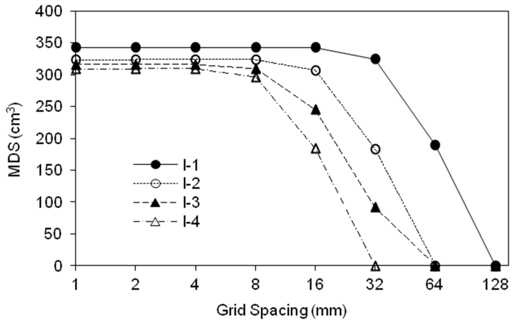
The relationships between grid size and MDS for Surfaces I-1–I-4 are shown in Figure 4. The MDS values were constant for smaller grid sizes (∆d < 4 mm) for all four surfaces. That is, there was a range of grid sizes, within which MDS did not change or only had minor changes. Such a range of grid sizes could vary, depending on the surface topographic characteristics. This information can be used to determine the “best” representative DEM resolution for hydrologic modeling and analysis. As the grid size increased, different surfaces exhibited dissimilar MDS decreasing patterns due to the changes in DEM representations and the loss of surface topographic details (Figure 4). Eventually, the MDS of a surface decreased to zero at a certain grid size (
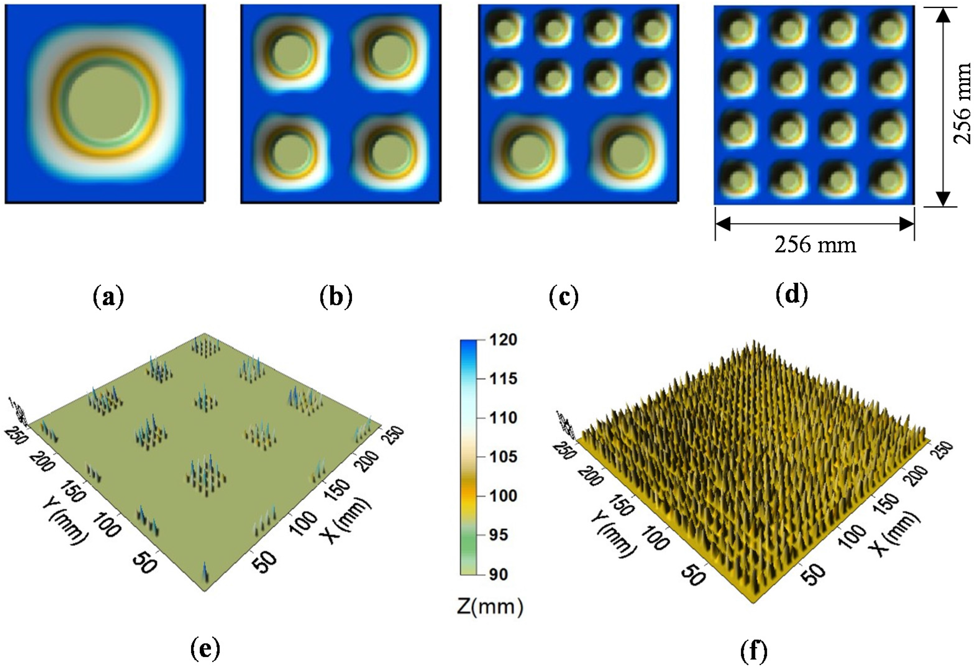
Figure 4). The grid size corresponding to the zero MDS depended on the surface topographic characteristics (e.g., number, shape and size of puddles). As expected, the surfaces with smaller depressions (e.g., Surface I-4, Figure 1d) were more sensitive to the change in grid size, showing an earlier decrease in MDS and a smaller zero-MDS grid size. Surface I-1 with the single largest depression (Figure 1a) had the greatest zero-MDS grid size (Figure 4). The maximum grid sizes for Surfaces I-1–I-4 were 128, 64, 64 and 32 mm, respectively (Figure 4).
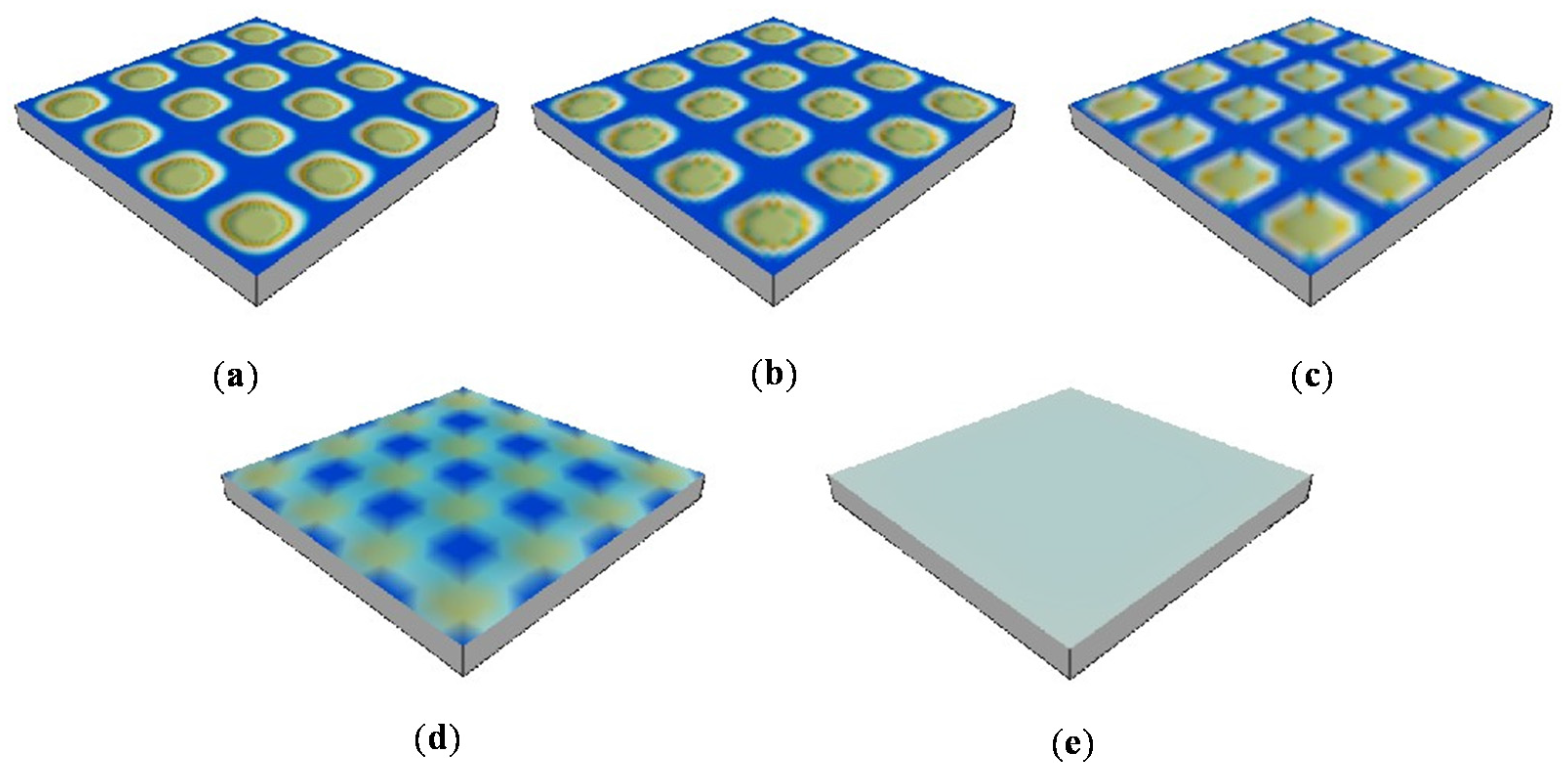
Figure 5 shows the changes in DEM representations and the loss of topographic detail for Surface I-4 (Figure 1d; 16 puddles) induced by the changes in DEM resolution (grid sizes ∆d increased from 2 to 4, 8, 16 and 32 mm). The depression storage gradually decreased with an increase in grid spacing. As a result, Surface I-4 was smoothened out, eventually resulting in a zero MDS at the largest grid size ∆d = 32 mm (Figure 5e). This example demonstrates the significant influence of DEM resolution on the topographic properties of a surface and related parameters (e.g., MDS) that are often used for hydrologic and environmental modeling.
Figure 4. Relationships of grid spacing and maximum depression storage (MDS) determined by the averaging interpolation method for ideal Surfaces I-1–I-4.
Water 07 02293 g004
Figure 5. Demonstration of the loss of surface topographic details determined by the averaging interpolation method for ideal Surface I-4: (a) ∆d = 2 mm; (b) ∆d = 4 mm; (c) ∆d = 8 mm; (d) ∆d = 16 mm; (e) ∆d = 32 mm.
Water 07 02293 g005
The above analyses revealed that due to the loss of surface topographic detail, MDS decreased with an increase in grid size, and correspondingly, the number of puddles also decreased. This finding is similar to the one from Huang and Bradford [7], but different from several other researchers [3,8,
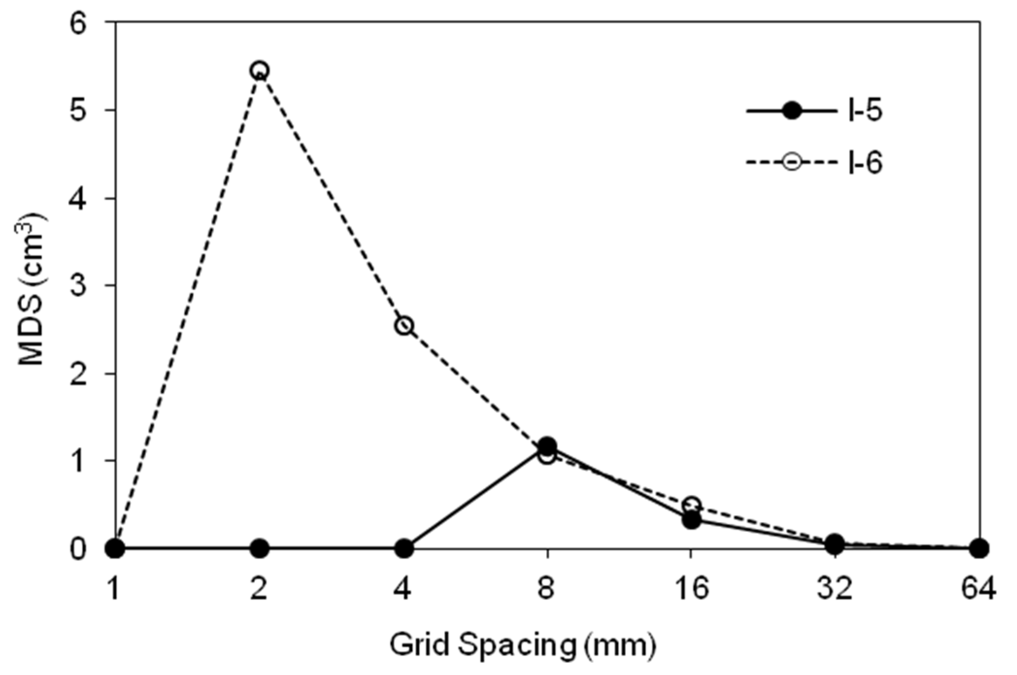
9]. To verify the related conclusions and to better understand the underlying reasons, Surfaces I-5 and I-6 (Figure 1e,f) were used for further testing. As shown in Figure 6, MDS increased with an increase in the grid spacing for both surfaces, indicating that certain artificial depressions were created during the interpolation/aggregation process, which further affected the computed depression storage. However, the MDS of Surface I-5 started to increase beyond ∆d = 4 mm. Then, MDS gradually decreased down to zero at ∆d = 64 mm for both surfaces (Figure 6). Surface I-6 had much greater MDS values than Surface I-5 for smaller grid sizes (e.g., ∆d = 2 and 4 mm) (Figure 6). Hence, it can be concluded that the extent of the influence of DEM resolution on the MDS computation also depends on the surface topographic characteristics.
Figure 6. Relationships of grid spacing and maximum depression storage (MDS) determined by the averaging interpolation method for Surfaces I-5 and I-6.
Water 07 02293 g006
To better demonstrate how the “artificial depressions” were generated during the interpolation/aggregation process, the derived DEMs for a small portion of Surface I-5 for ∆d = 2, 4 and 8 mm were compared with the original DEM (∆d = 1 mm). As shown in Figure 7, for the grid sizes of 1–4 mm, the surfaces exhibited similar topographic features, such as peaks and a zero MDS, although the peaks were at different elevations for the three surfaces (Figure 7a–c). However, an artificial puddle was formed when the grid size was increased to 8 mm (Figure 7d), which resulted in a non-zero MDS. In summary, as DEM grid sizes change, “artificial puddles” can be created, and real small puddles may disappear, which consequently alters the surface topographic characteristics. This helps explain why different researchers (e.g., [3,8,9]) reached distinct conclusions concerning the effects of DEM resolution on MDS.
Figure 7. Demonstration of the generation of “artificial puddles” using the averaging interpolation method for a portion of Surface I-5: (a) ∆d = 1 mm; (b) ∆d = 2 mm; (c) ∆d = 4 mm; (d) ∆d = 8 mm.
Water 07 02293 g007

3.2. DEM Resolution Effects for Laboratory-Scale Soil Surfaces

The puddle delineation results for Surfaces II-1 and II-2 (Figure 2a,b) are shown in Figure 8. The NP decreased quickly with an increase in grid spacing due to the loss of microrelief detail (Figure 8a). For example, as grid spacing increased from 2 to 3 mm, Surfaces II-1 and II-2 lost 2235 and 283 puddles, respectively. Both MDS and MPA of Surfaces II-1 and II-2 decreased with an increase in grid spacing and eventually approached zero (Figure 8b,c). The MDS and MPA of the smoother Surface II-1 decreased more quickly than the rougher Surface II-2 (Figure 8b,c). The variations in the MDS of Surface II-2 at ∆d = 80 and 100 mm (Figure 8b) can be attributed to certain “artificial puddles” generated during the aggregation process. The MDS and MPA approached zero at ∆d = 30 and 200 mm for Surfaces II-1 and II-2, respectively (Figure 8b,c).
Figure 8. Relationships of grid spacing and (a) the number of puddles (NP); (b) the maximum depression storage (MDS) and (c) the maximum ponding area (MPA) determined by using the kriging method and the PD software for Surfaces II-1 and II-2.
Water 07 02293 g008

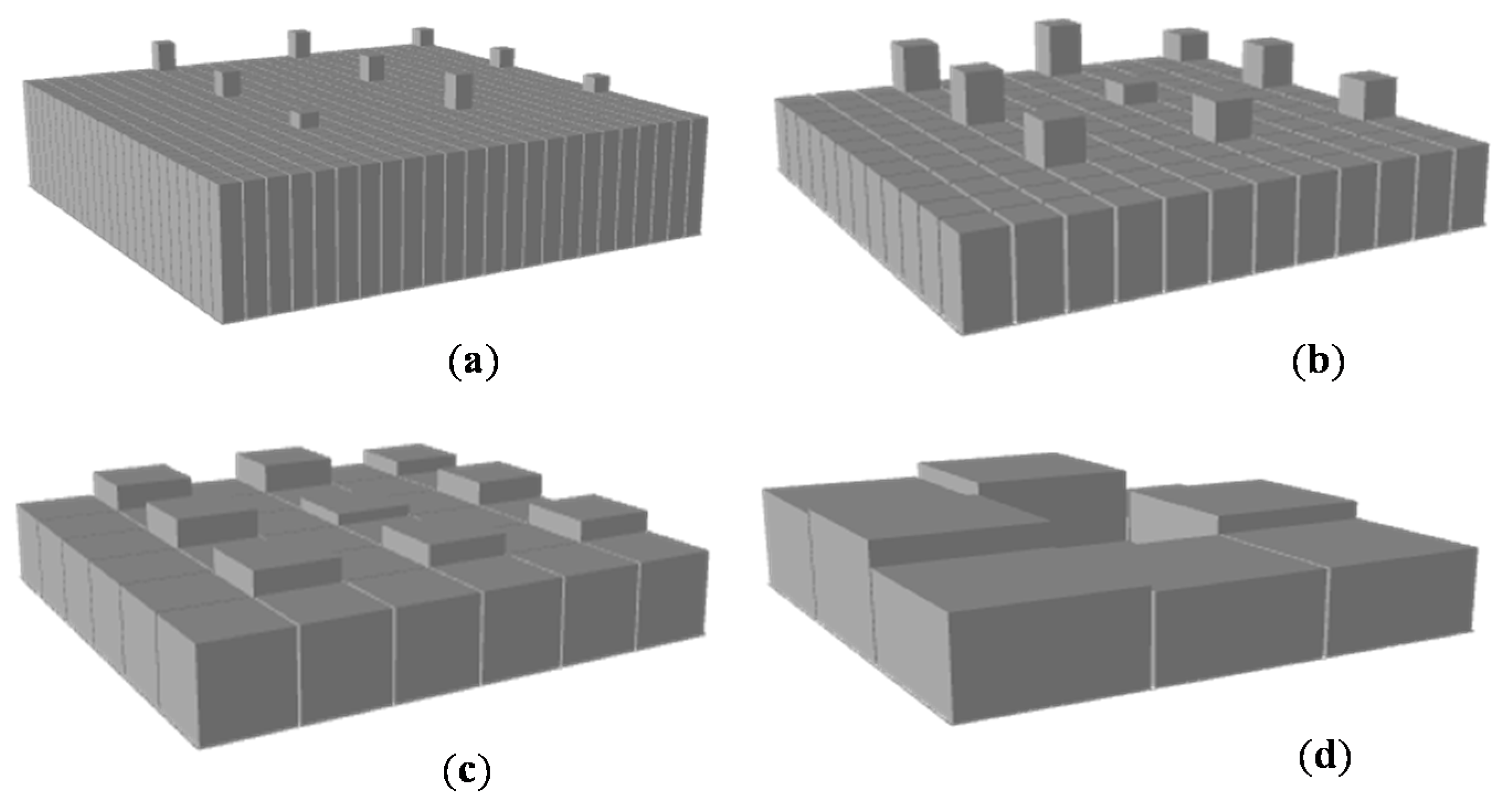
3.3. DEM Resolution Effects for Watershed-Scale Surfaces

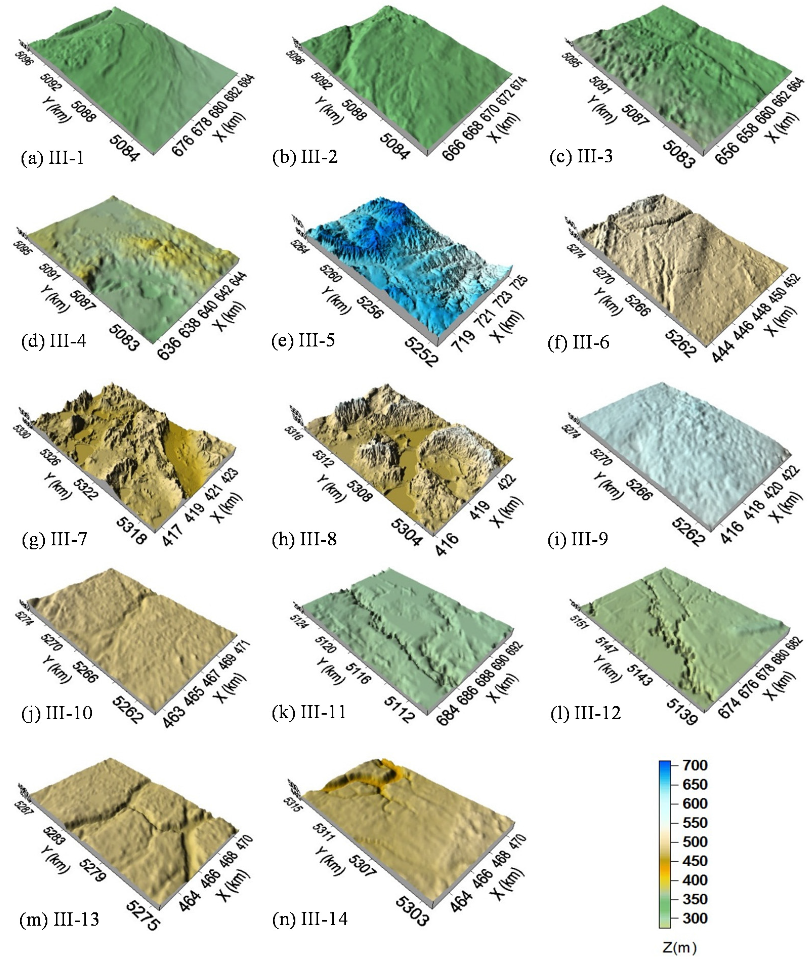
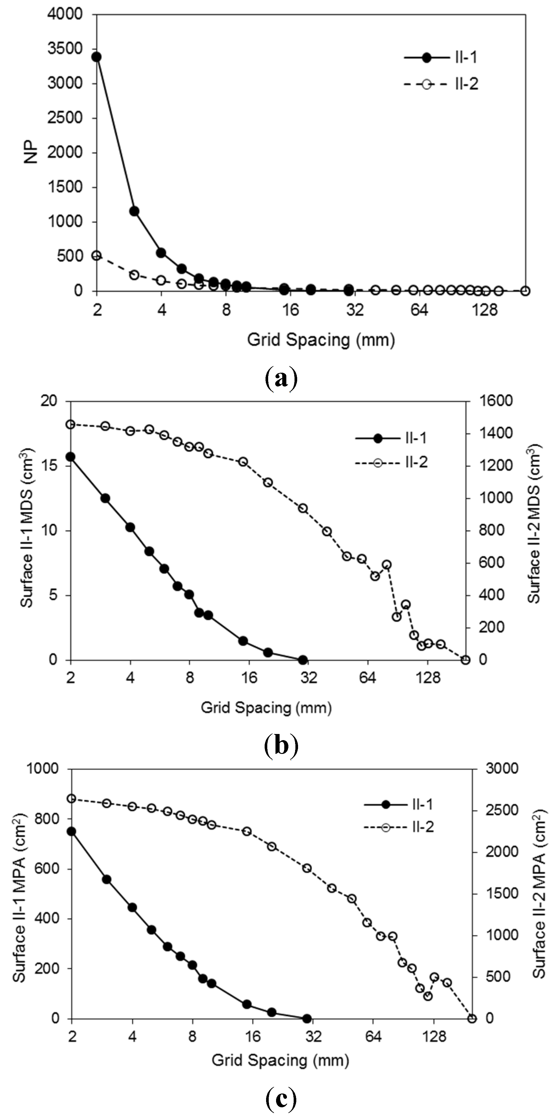
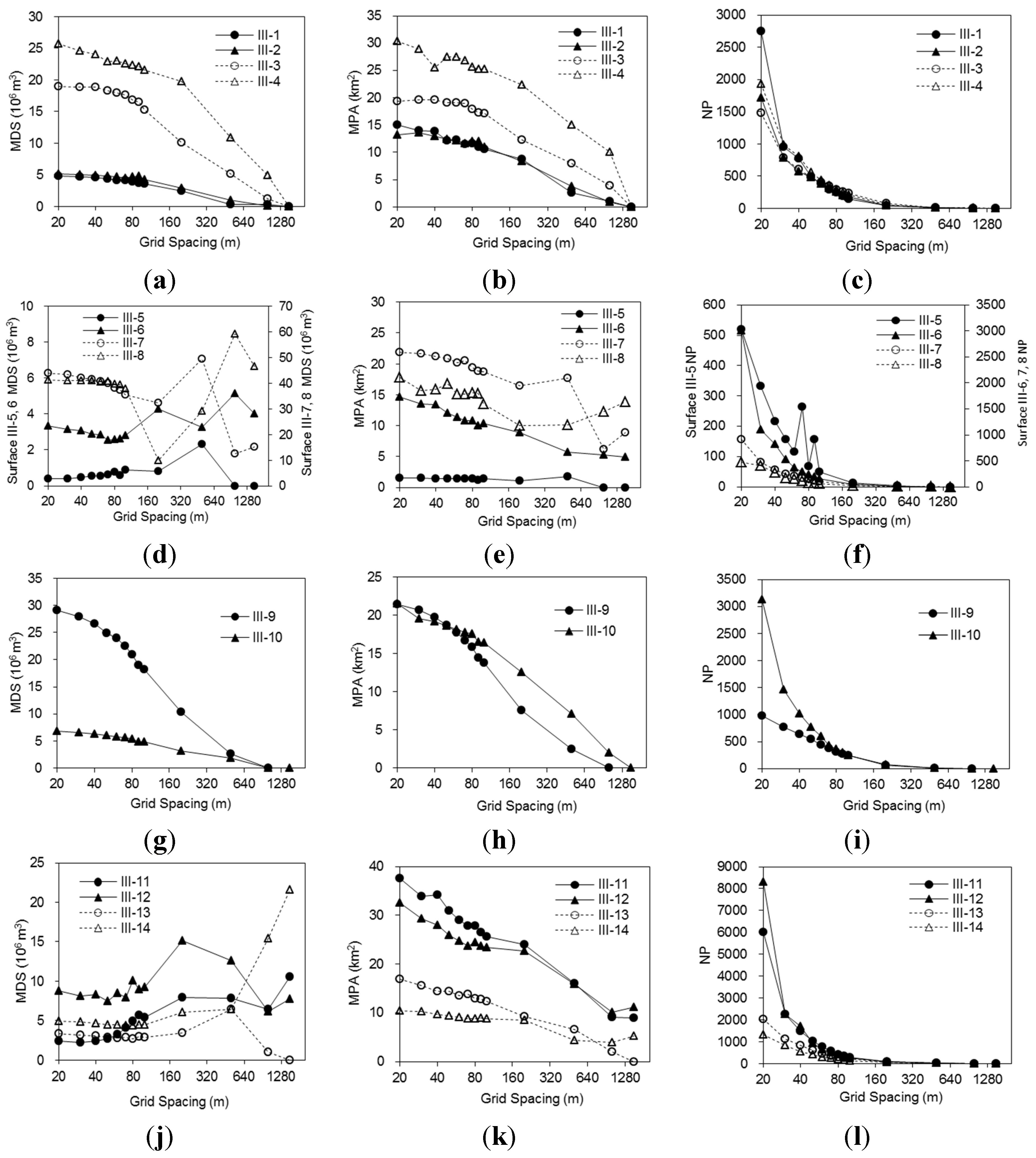
Figure 9 shows the comparison between grid spacing and MDS, MPA and NP for the watershed-scale Surfaces III-1–III-14 (Figure 3). Dissimilar changing patterns of MDS, MPA and NP can be observed for these fourteen surfaces (Figure 9). For Surfaces III-1–III-4, MDS and MPA decreased with increasing grid spacing and approached zero at ∆d = 1280 m (Figure 9a,b). As expected, the rougher Surfaces III-3 and III-4 had greater MDS and MPA values. The NP values of Surfaces III-1–III-4 decreased rapidly with an increase in grid spacing (Figure 9c). These findings were similar to the results for the laboratory-scale soil surfaces shown in Figure 8.
Figure 9. Relationships of grid spacing and maximum depression storage (MDS), maximum ponding area (MPA) and number of puddles (NP) determined by using the kriging method and the PD software for Surfaces III-1–III-14.
Water 07 02293 g009
For Surfaces III-5–III-8, however, their MDS and MPA values varied with an increase in the grid size (Figure 9d,f). The MDS and MPA of Surface III-5 increased initially, reached the maximum values at ∆d = 500 m and then decreased to zero at ∆d = 1000 m (Figure 9d,e). The MDS of Surface III-6 varied with grid spacing (Figure 9d), while its MPA exhibited a decreasing pattern (Figure 9e). Surfaces III-7a and III-8 displayed significant variations in both MDS and MPA as the grid size changed. The NP curves of Surfaces III-5–III-8 showed an overall decreasing pattern as the grid size increased. However, the NP of Surface III-5 displayed some variations at ∆d = 70–90 m (Figure 9f). This can be attributed to the “unreal” depressions induced during the interpolation/aggregation process. Comparisons of the MDS, MPA and NP between the four plain surfaces (III-1–III-4) (Figure 9a–c) and the four mountain-type surfaces (III-5–I III-8) (Figure 9d–f) suggested that the changing patterns of these topographic parameters with grid spacing were different, primarily depending on their topographic characteristics.
Comparison between Surfaces III-9 (Figure 3i) and III-10 (Figure 3j) revealed some interesting results. The elevations of Surface III-9 varied in a greater range from 511.4 to 620.3 m (i.e., the difference was 108.9 m), while the elevations of Surface III-10 ranged from 475.3 to 508.5 m (the difference was only 33.2 m). As expected, the MDS of Surface III-9 was much greater than that of Surface III-10 (Figure 9g). However, both surfaces had very comparable MPA curves (both quantity and distribution) (Figure 9h). Like Surfaces III-1–III-4 (Figure 9c), the NP curves of Surfaces III-9 and III-10 also showed a decreasing trend with increasing grid spacing, even though Surface III-10 included more depressions (Figure 9i).
Similar to Surfaces III-7 and III-8 (Figure 9d), Surfaces III-11–III-12 also showed substantial variability in their MDS (Figure 9j). The changing pattern of MDS for Surface III-13 (Figure 9j) was similar to that of Surface III-5 (Figure 9d), and its MDS reached zero at ∆d = 1500 m. In contrast, Surface III-14 showed a significant increase in MDS, especially for ∆d > 500 m, and eventually reached the highest MDS at the coarsest resolution (∆d = 1500 m) (Figure 9j). The MPA values of Surfaces III-11–III-12 were greater than those of Surfaces III-13 and III-14, and the four MPA curves exhibited an overall decreasing trend with increasing grid spacing (Figure 9k). Similar to Surfaces III-1–III-4 (Figure 9c), substantial decreases can be observed in the NP curves of Surfaces III-11–III-14, as the grid size increased (Figure 9l).
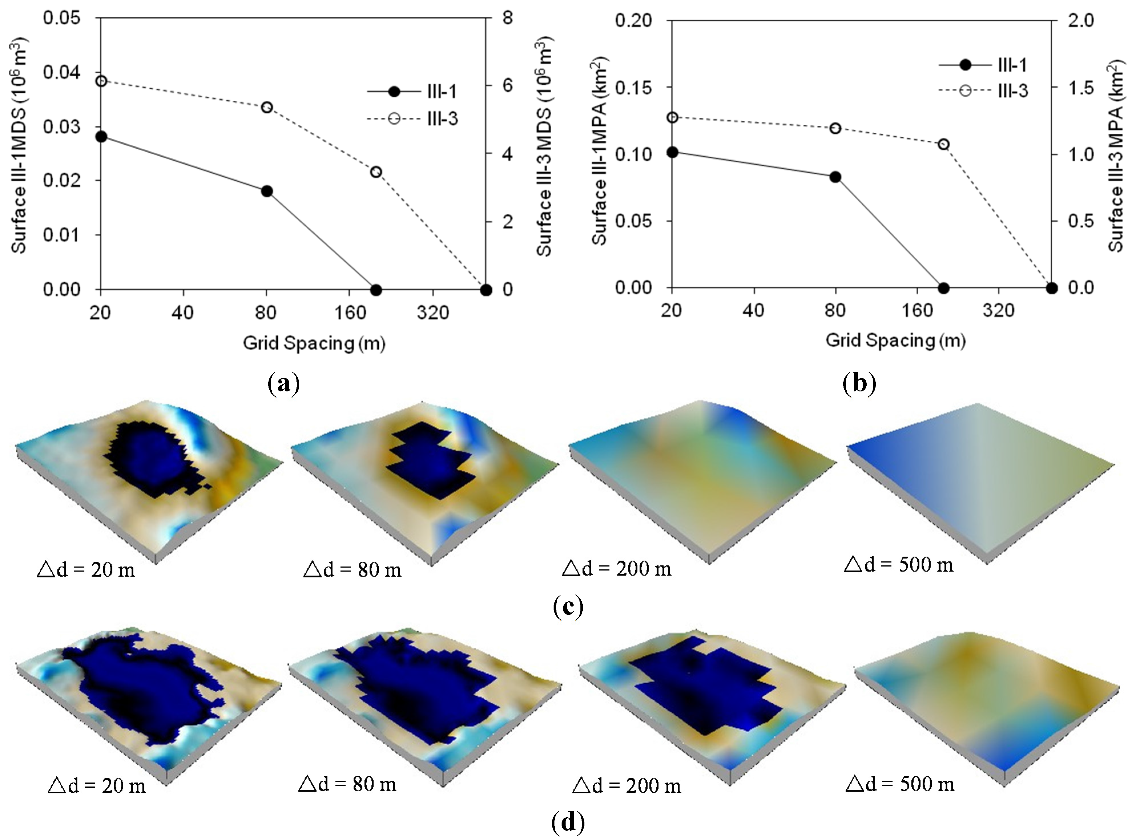
To look into more detail at the alteration of DEM representations and the loss of topographic detail due to the changes in DEM resolution, a portion of the plain-type Surfaces III-1 and III-3 (zoomed-in areas) and four different grid sizes (∆d = 20, 80, 200 and 500 m) were selected, and the changes in their MDS and MPA values were analyzed. Figure 10a,b respectively show the changes in their MDS and MPA. Basically, both MDS and MPA decreased with increasing grid size. As a result, the puddles/depressions on Surfaces III-1 and III-3 were smoothened out, eventually resulting in a zero depression storage (Figure 10c,d). The MDS and MPA became zero (i.e., no depression/puddle) at ∆d = 200 m for Surface III-1 (Figure 10a–c) and at ∆d = 500 m for Surface III-3 (Figure 10a,b,d). The above analyses revealed that due to the loss of surface topographic detail, MDS and MPA decreased with an increase in grid size, and correspondingly, the number of depressions/puddles also decreased. Similar to the small-scale surfaces (Figure 4), MDS and MPA appeared to be changed insignificantly for smaller grid sizes (∆d < 80 m). Again, this finding can be useful for multi-scale hydrologic modeling and analysis.
Figure 10. Demonstration of the loss of surface topographic details (maximum depression storage MDS and maximum ponding area MPA) determined by the kriging method and the PD software for Surfaces III-1 and III-3: (a) MDS; (b) MPA; (c) Surface III-1; (d) Surface III-3.
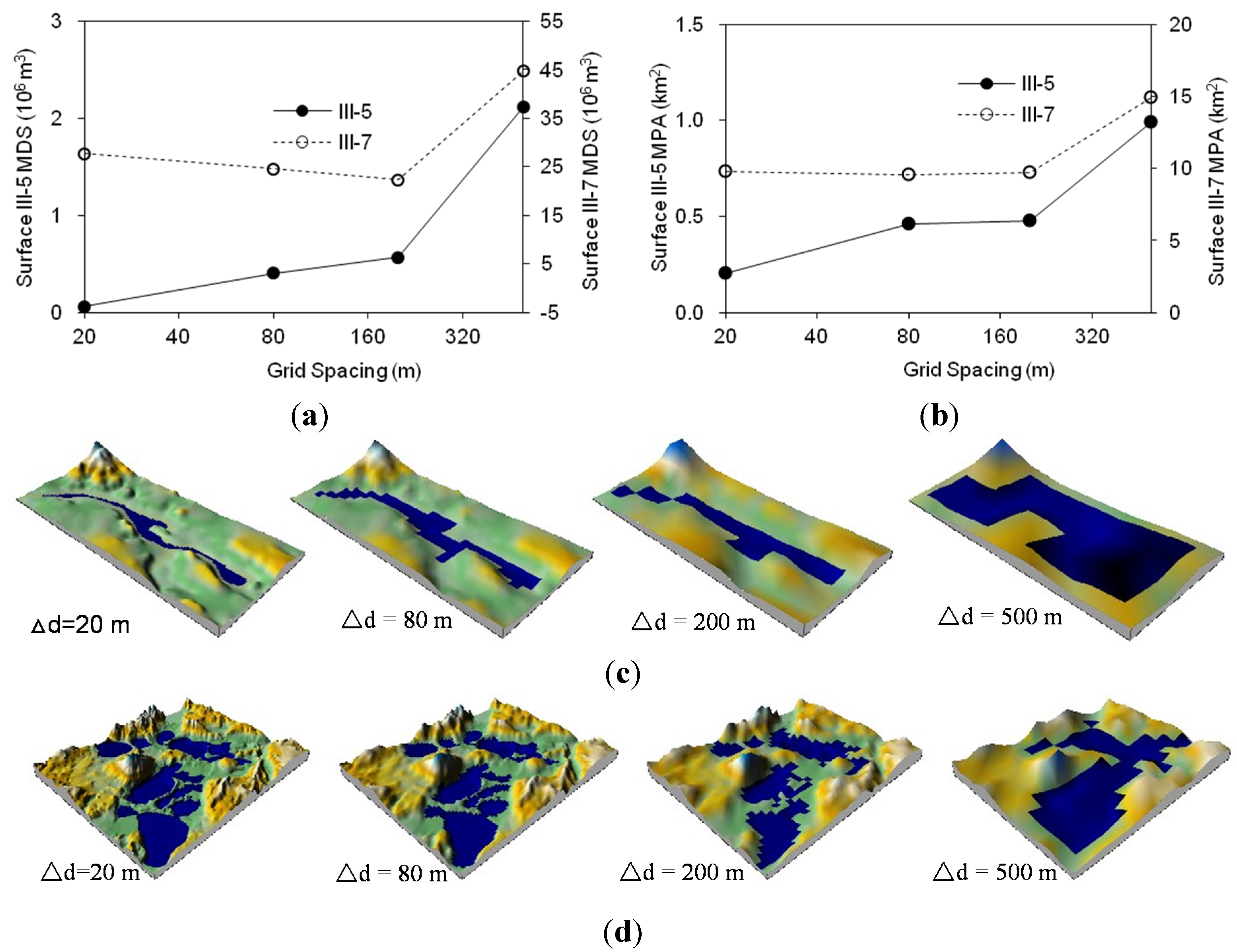
Water 07 02293 g010
Figure 11a and Figure 11b respectively show the changes in MDS and MPA for a selected portion of the mountain-type Surfaces III-5 and III-7, while Figure 11c and Figure 11d display the delineated surfaces and puddle distributions for the four different resolutions (∆d = 20, 80, 200 and 500 m). Different from the selected plain Surfaces III-1 and III-3 (Figure 10a,b), as the grid size increased from 20 to 500 m, the MDS and MPA of the small piece of Surface III-5 increased from 0.06 × 10⁶ to 2.11 × 10⁶ m3 and from 0.20 to 0.99 km2, respectively (Figure 11a,b). Figure 11c also shows increases in the MDS and MPA. The MDS and MPA of the small piece of Surface III-7 displayed slight decreases for smaller grid sizes (∆d ≤ 200 m) and then increased to 44.68 × 10⁶ m3 and 14.89 km2, respectively (Figure 11a,b). Such changing trends of MDS and MPA also can be observed in Figure 11d. This result suggested that the computation of MDS was strongly affected by DEM resolution and the complexity of surface topography. The changes in the computed topographic parameters can be attributed to the introduced artificial depressions and the smoothing effects.
Figure 11. Demonstration of the changes of surface topographic characterization (maximum depression storage MDS and maximum ponding area MPA) determined by the kriging method and the PD software for Surfaces III-5 and III-7: (a) MDS; (b) MPA; (c) Surface III-5; (d) Surface III-7.
Water 07 02293 g011
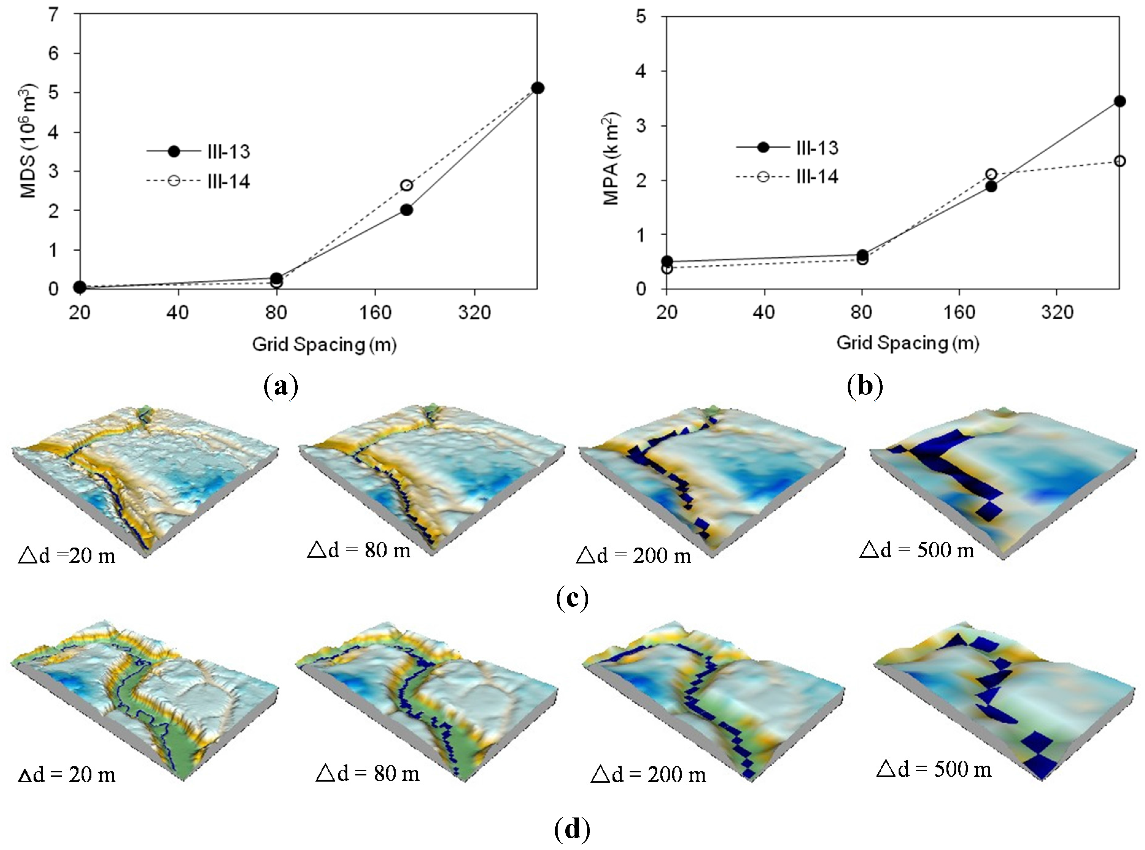
Figure 12a,b shows the changes in the MDS and MPA of the selected pieces of Surfaces III-13 and III-14 that were characterized by river channels. As the grid size increased from 20 to 500 m, the MDS and MPA of the small piece of Surface III-13 increased from 0.04 × 10⁶ to 5.11 × 10⁶ m3 and from 0.51 to 3.46 km2, respectively (Figure 12a,b). Such increases in the MDS and MPA also can be observed in Figure 12c. The MDS and MPA of the selected piece of Surface III-14 also increased from 0.07 × 10⁶ to 5.13 × 10⁶ m3 and from 0.39 to 2.35 km2, respectively (Figure 12a,b,d). This analysis, again, demonstrates the dominant role of surface topography and DEM resolution in the computation of topographic parameters.

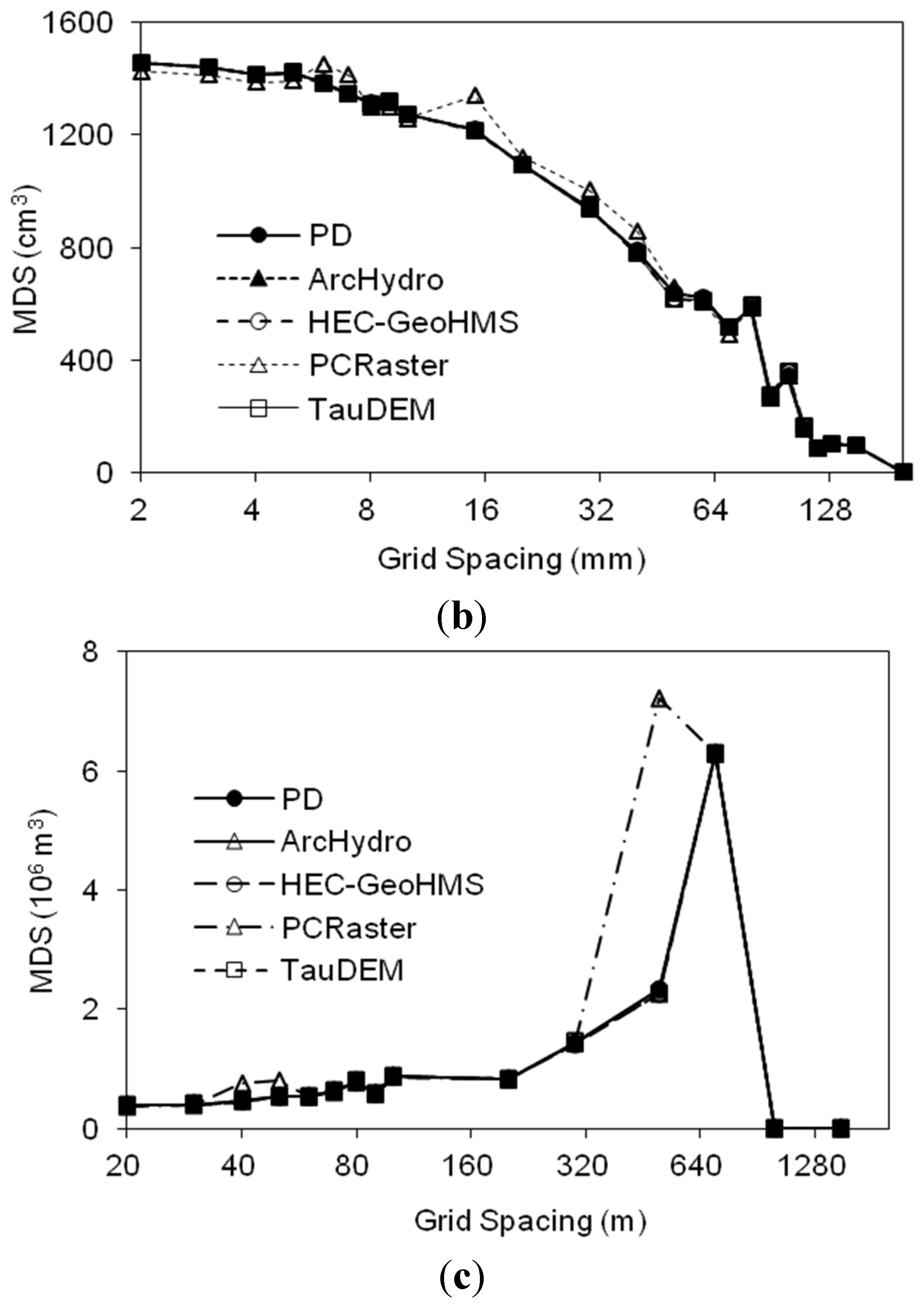
3.4. Influences of Different Delineation Methods

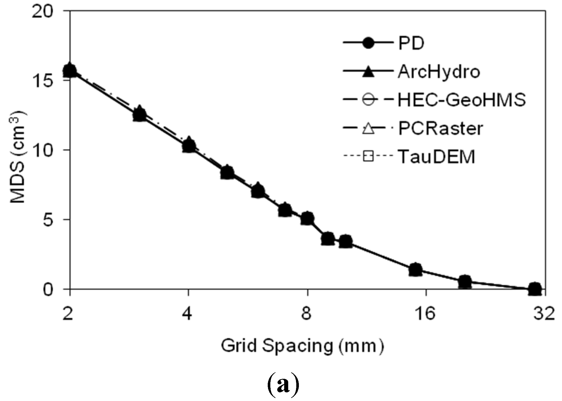
Figure 13 shows the comparison of MDS values calculated by the PD, ArcHydro, HEC-GeoHMS, PCRaster and TauDEM software packages for varying resolution DEMs of the laboratory Surfaces II-1 and II-2 (Figure 2a,b), as well as the watershed-scale Surface III-5 (Figure 3e). For the laboratory-scale smooth Surface II-1 (Figure 2a), the five programs yielded almost identical MDS values for all grid sizes (Figure 13a), showing that the MDS values decreased with increasing DEM grid size. For the laboratory-scale rough Surface II-2, the MDS values from the five programs followed similar decreasing patterns with an increase in the grid size. However, the MDS curve from PCRaster exhibited minor differences at certain grid size points (Figure 13b). The MDS values were close to zero at ∆d = 200 mm for all five methods (Figure 13b). For the watershed-scale Surface III-5, a significant difference in MDS can be observed at ∆d = 500 m (Figure 13c). For Surface III-5, PCRaster yielded a peak MDS (7.23 × 10⁶ m3) at ∆d = 500 m, while the four other programs reached a peak MDS (6.29 × 10⁶ m3) at ∆d = 700 m (Figure 13c).
Figure 12. Demonstration of the changes of surface topographic characterization (maximum depression storage MDS and maximum ponding area MPA) determined by the kriging method and the PD software for Surfaces III-13 and III-14: (a) MDS; (b) MPA; (c) Surface III-13; (d) Surface III-14.
Water 07 02293 g012
Figure 13. Relationships of grid spacing and maximum depression storage (MDS) determined by the PD, ArcHydro, HEC-GeoHMS, PCRaster and TauDEM software packages for: (a) Surface II-1; (b) Surface II-2; (c) Surface III-5.
Water 07 02293 g013aWater 07 02293 g013b
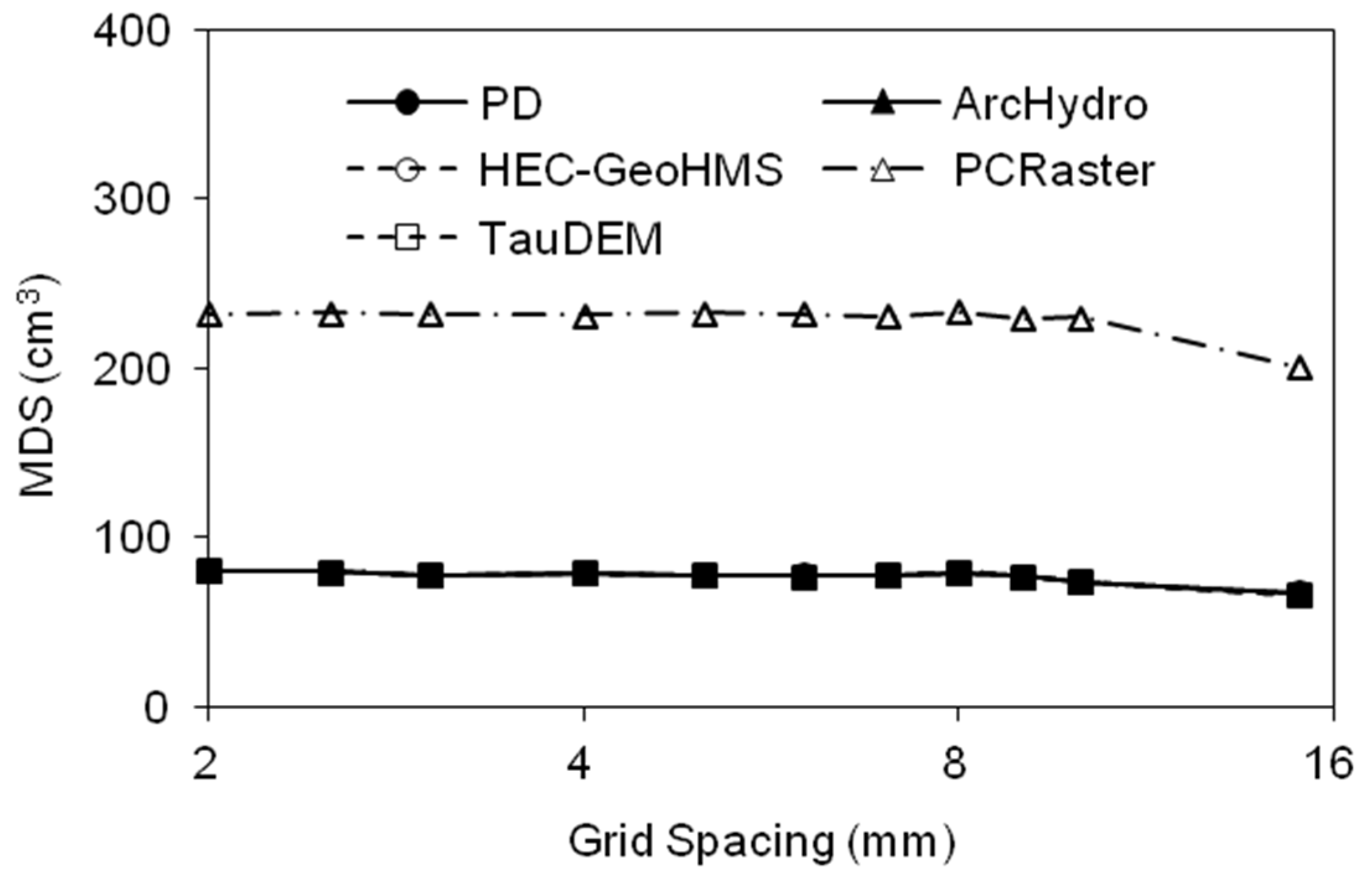
Boundary conditions (e.g., closed or open boundaries) often affect the computation of MDS in a surface delineation program [8]. This boundary-related issue involves how to deal with the depressions adjacent to surface boundaries and computation of related depression storages. Surface II-3 (Figure 2c), featuring four major boundary depressions/puddles, was used to address this issue. Based on the original DEM of Surface II-3, eleven coarser resolution DEMs (∆d = 2–15 mm) were generated for this study. PD, ArcHydro, PCRaster, HEC-GeoHMS and TauDEM were applied to compute the MDS of this laboratory surface. As shown in Figure 14, PCRaster yielded much higher MDS values for all grid sizes, and the MDS remained nearly steady (Figure 14). This can be attributed to the fact that a closed boundary condition was assumed in PCRaster. The four other programs provided similar MDS values, which were nearly constant for all grid sizes (Figure 14). The aforementioned results suggest that different methods can be utilized in the surface delineation programs to deal with the boundary depressions or incomplete depressions/puddles, which could lead to different results. It is critical to fully understand the underlying assumptions in the programs.
Figure 14. Relationships of grid spacing and maximum depression storage (MDS) determined by the PD, ArcHydro, HEC-GeoHMS, PCRaster and TauDEM software packages for Surface II-3 with boundary puddles.
Water 07 02293 g014
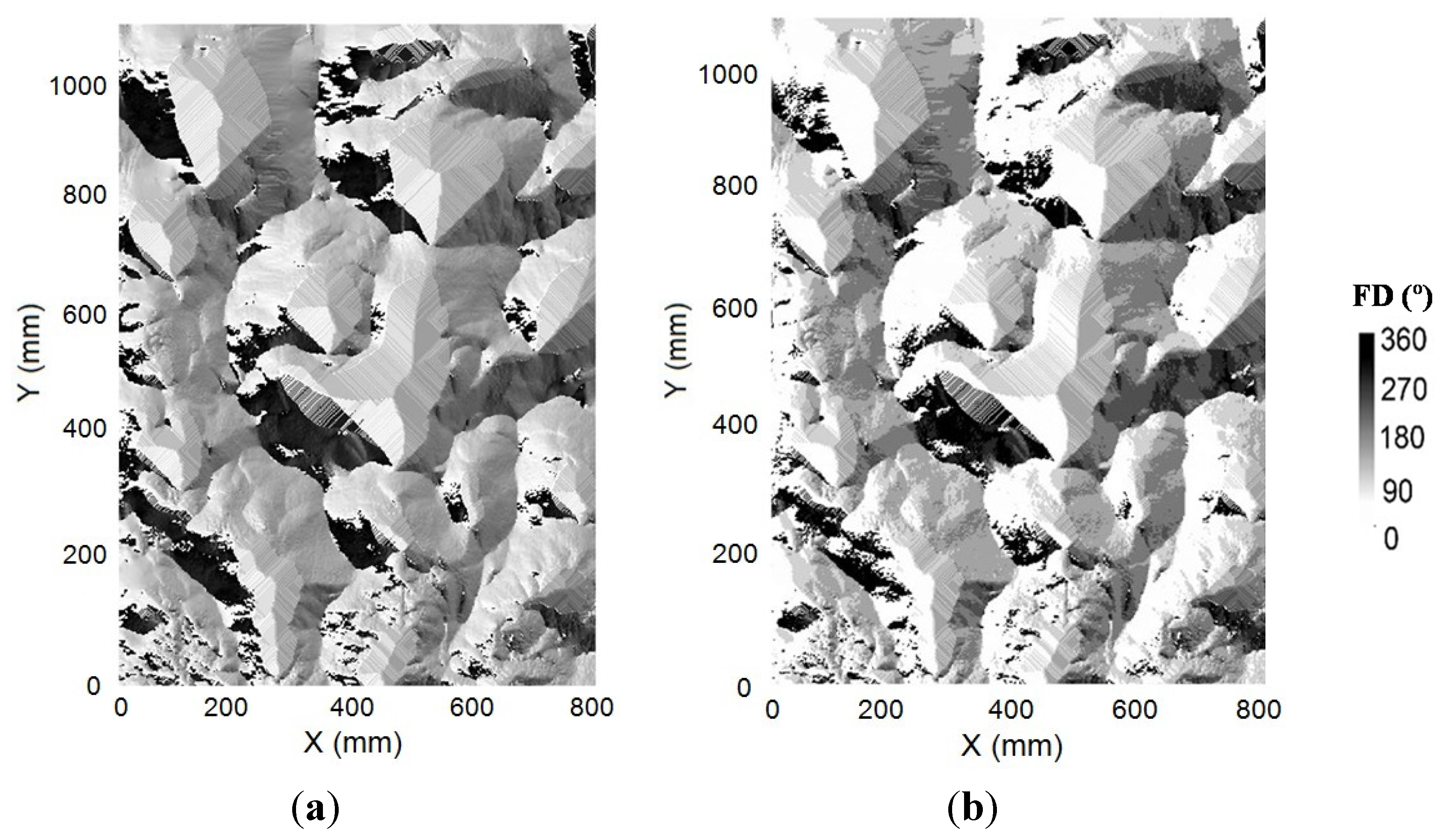
For various DEM resolutions, TauDEM yielded MDS values similar to those from PD, ArcHydro and HEC-GeoHMS. However, the D8 and D-infinity methods resulted in dissimilar flow directions. For comparison purposes, the eight flow directions from the D8 method were converted to angles (east: 0°; northeast: 45°; north: 90°; northwest: 135°; west: 180°; southwest: 225°; south: 270°; southeast: 315°). Figure 15 shows the comparison of flow directions determined by the D-infinity and D8 methods for the laboratory Surface II-2 (Figure 2b) and the watershed Surface III-5 (Figure 3e). Although the overall distributions and changing patterns of flow directions from the two methods were similar for both surfaces (II-2 and III-5), the D-infinity method did provide more grey scales (i.e., more flow directions). Additionally, certain discrepancies in flow directions at many local areas can be observed for both laboratory and watershed surfaces (
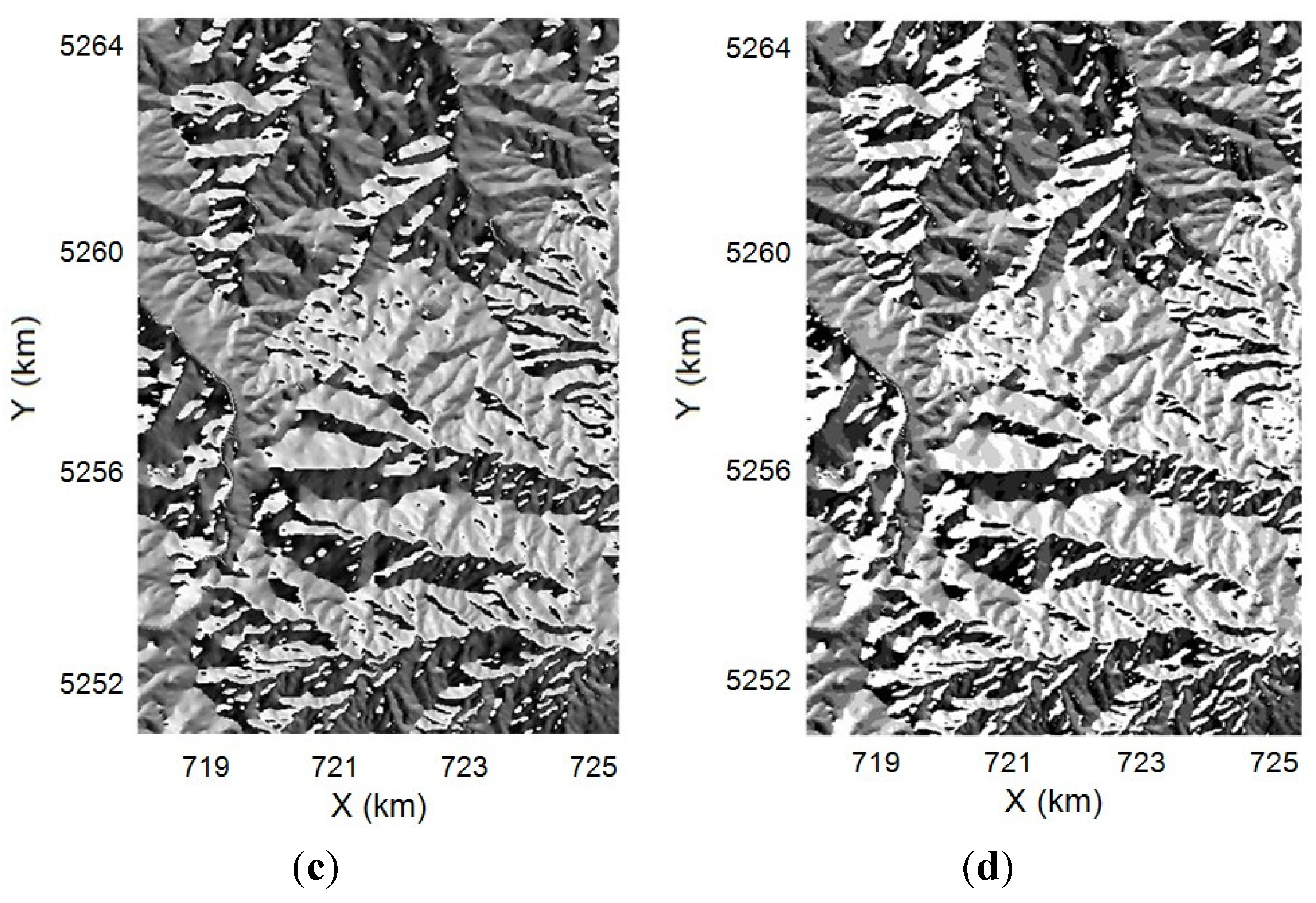
Figure 15). These differences and variations in flow directions would potentially alter flow accumulations and hydrologic connectivity and further affect watershed modeling.
Figure 15. Comparison of flow directions computed by the D8 and D-infinity methods for laboratory Surface II-2 and watershed Surface III-5: (a) Surface II-2, D-infinity; (b) Surface II-2, D8; (c) Surface III-5, D-infinity; (d) Surface III-5, D8.
Water 07 02293 g015aWater 07 02293 g015b

4. Conclusions

In this study, we systematically evaluated the impacts of DEM resolution on puddle characterization and computation of topographic parameters (e.g., MDS, MPA and NP) by analyzing the related influence factors, including surface topography and surface delineation methods. Twenty-three surfaces with varying spatial scales and topographic characteristics (including ideal artificial surfaces, laboratory-scale soil surfaces and real watershed-scale land surfaces) were selected and delineated by using five different methods/software packages: PD, ArcHydro, HEC-GeoHMS, PCRaster and TauDEM. Their performances in the computation of MDS were compared and evaluated.
For most small-scale surfaces (e.g., the ideal Surfaces I-1–I-4 and the laboratory soil Surfaces II-1–II-2) and watershed-scale plain-type surfaces (e.g., III-1–III-4), their computed MDS, MPA and NP values decreased with an increase in DEM grid spacing. This changing pattern primarily can be attributed to the smoothing effect for coarser resolution DEMs. For some special surfaces with topographic peaks, however, their MDS values increased initially, reached a maximum value and then decreased, which was mainly attributed to “unreal” depressions/puddles generated during the DEM interpolation/aggregation process. The MDS, MPA and NP of the watershed-scale mountain-type surfaces that had a wide range of elevations showed a distinct changing pattern, featuring significant variations with grid spacing, which can be attributed to both the smoothing effect and the artificial depressions from the interpolation/aggregation process. In addition, a certain threshold of DEM grid size existed for most surfaces, beyond which significant changes in topographic properties were observed. Such a DEM grid threshold varied depending on the real surface topographic characteristics (e.g., size and distribution of depressions/puddles). This information about the DEM scale can be useful for selecting the effective or “optimal” DEM resolution for hydrologic and environmental modeling. Development of mathematical relationships between DEM resolution and topographic parameters, quantification of the DEM representation scale and surface roughness scale and identification of the optimal DEM resolution are of both theoretical and practical importance. Some relevant studies (e.g., [24]) have been performed. As an important future research direction, however, more efforts are needed to fully address this issue. In summary, DEM resolution had significant impacts on the characterization and quantification of surface topography. In the meantime, it should be emphasized that the extent and significance of the DEM resolution effect also depended on the complexity and variability of surface topography.
It was found that the PD, ArcHydro, HEC-GeoHMS and TauDEM programs provided similar delineation results and comparable topographic parameters for both large- and small-scale surfaces. However, due to the different methods used for boundary depressions/puddles (closed boundary approach), PCRaster yielded much higher MDS values for surfaces with boundary depressions/puddles. The D-infinity method in TauDEM provided improved the computation of flow directions, which had potential to further improve the quantification of flow accumulations and watershed modeling.

Acknowledgments

This material is based upon work supported by the National Science Foundation under Grant No. EAR-0907588 and NSF Experimental Program to Stimulate Competitive Research (EPSCoR) Award IIA-1355466. The authors would like to thank Jun Yang and Jessica Nelis for their contributions to the related work.

Author Contributions

Both authors contributed equally to this work, including the related research and writing.

Conflicts of Interest

The authors declare no conflict of interest.

References

  1. Ullah, W.; Dickinson, W.T. Quantitative description of depression storage using a digital surface model. I determination of depression storage. J. Hydrol. 1979, 42, 63–75. [Google Scholar] [CrossRef]
  2. Darboux, F.; Davy, P.; Gascuel-Odoux, C.; Huang, C. Evolution of soil surface roughness and flowpath connectivity in overland flow experiments. Catena 2001, 46, 125–139. [Google Scholar] [CrossRef]
  3. Abedini, M.J.; Dickinson, W.T.; Rudra, R.P. On depressional storages: The effect of DEM spatial resolution. J. Hydrol. 2006, 318, 138–150. [Google Scholar] [CrossRef]
  4. Hansen, B. Estimation of surface runoff and water-covered area during filling of surface microrelief depressions. Hydrol. Process. 2000, 14, 1235–1243. [Google Scholar] [CrossRef]
  5. Govers, G.; Takken, I.; Helming, K. Soil roughness and overland flow. Agronomie 2000, 20, 131–146. [Google Scholar] [CrossRef]
  6. Darboux, F.; Huang, C. An instantaneous-profile laser scanner to measure soil surface microtopography. Soil Sci. Soc. Am. J. 2003, 67, 92–99. [Google Scholar] [CrossRef]
  7. Huang, C.; Bradford, J.M. Depressional storage for Markov-Gaussian surfaces. Water Resour. Res. 1990, 26, 2235–2242. [Google Scholar] [CrossRef]
  8. Kamphorst, E.C.; Jetten, V.; Guerif, J. Predicting depressional storage from soil surface roughness. Soil Sci. Soc. Am. J. 2000, 64, 1749–1758. [Google Scholar] [CrossRef]
  9. Kamphorst, E.C.; Duval, Y. Validation of a numerical method to quantify depression storage by direct measurements on moulded surfaces. Catena 2001, 43, 1–14. [Google Scholar] [CrossRef]
  10. Kamphorst, E.C.; ChadKuf, J.; Jetten, V.; Guerif, J. Generating 3D soil surfaces from 2D height measurements to determine depression storage. Catena 2005, 62, 189–205. [Google Scholar] [CrossRef]
  11. Moore, I.D.; Larson, C.L. Estimating micro-relief surface storage from point data. Trans. ASAE 1979, 22, 1073–1077. [Google Scholar] [CrossRef]
  12. Jenson, S.K.; Domingue, J.O. Extracting topographic structure from digital elevation data for geographic information systems analysis. Photogramm. Eng. Remote Sens. 1988, 54, 1593–1600. [Google Scholar]
  13. Martz, L.M.; Garbrecht, J. Automated extraction of drainage network and watershed data from digital elevation models. Water Resour. Bull. 1993, 29, 901–908. [Google Scholar] [CrossRef]
  14. Garbrecht, J.; Martz, L.W. TOPAZ: An Automated Digital Landscape Analysis Tool for Topographic Evaluation, Drainage Identification, Watershed Segmentation and Subcatchment Parameterization: Overview; ARS-NAWQL 95–1; United States Department of Agriculture, Agricultural Research Service (USDA-ARS): Durant, OK, USA, 1997.
  15. Martz, L.M.; Garbrecht, J. An outlet breaching algorithm for the treatment of closed depressions in a raster DEM. Comput. Geosci. 1999, 25, 835–844. [Google Scholar] [CrossRef]
  16. Planchon, O.; Darboux, F. A fast, simple and versatile algorithm to fill the depressions of digital elevation models. Catena 2001, 46, 159–176. [Google Scholar] [CrossRef]
  17. Maidment, D.R. Arc Hydro: GIS for Water Resources; ESRI Press: Redlands, CA, USA, 2002. [Google Scholar]
  18. User’s Manual, HEC-GeoHMS, Geospatial Hydrologic Modeling Extension; Version 4.2, CPD-77; U.S. Army Corps of Engineers, Hydrologic Engineering Center: Davis, CA, USA, 2009.
  19. User’s Manual, HEC-GeoHMS, Geospatial Hydrologic Modeling Extension; Version 10.1, CPD-77; U.S. Army Corps of Engineers, Hydrologic Engineering Center: Davis, CA, USA, 2013.
  20. Van Deursen, W.P.A.; Wesseling, C.G. The PC Raster package. Department of Physical Geography; Utrecht University: Utrecht, The Netherlands, 1992. [Google Scholar]
  21. Wesseling, C.G.; Karssenberg, D.; van Deursen, W.P.A.; Burrough, P.A. Integrating dynamic environmental models in GIS: The development of a dynamic modelling language. Trans. GIS 1996, 1, 40–48. [Google Scholar] [CrossRef]
  22. Carvajal, F.; Aguilar, M.A.; Aguera, F.; Aguilar, F.J.; Giraldez, J.V. Maximum depression storage and surface drainage network in uneven agricultural landforms. Biosyst. Eng. 2006, 95, 281–293. [Google Scholar] [CrossRef]
  23. Ullah, W.; Dickinson, W.T. Quantitative description of depression storage using a digital surface model. II Characteristics of surface depressions. J. Hydrol. 1979, 42, 77–90. [Google Scholar] [CrossRef]
  24. Yang, J.; Chu, X. Effects of DEM resolution on surface depression properties and hydrologic connectivity. J. Hydrol. Eng. 2013, 18, 1157–1169. [Google Scholar] [CrossRef]
  25. Vaze, J.; Teng, J.; Spencer, G. Impact of DEM accuracy and resolution on topographic indices. Environ. Model. Softw. 2010, 25, 1086–1098. [Google Scholar] [CrossRef]
  26. Yang, P.; Ames, D.P.; Fonseca, A.; Anderson, D.; Shrestha, R.; Glenn, N.F.; Cao, Y. What is the effect of LiDAR-derived DEM resolution on large-scale watershed model results? Environ. Model. Softw. 2014, 58, 48–57. [Google Scholar] [CrossRef]
  27. GIS Modules and Distributed Models of the Watershed; ASCE Task Committee on GIS Modules and Distributed Models of the Watershed; American Society of Civil Engineers: Reston, VA, USA, 1999.
  28. Tarboton, D.G.; Mohammed, I.N. TauDEM 5.1 Quick Start Guide to Using the TauDEM ArcGIS Toolbox. Available online: http://hydrology.usu.edu/taudem/taudem5/TauDEM51GettingStartedGuide.pdf (accessed on 27 April 2015).
  29. O’Callaghan, J.F.; Mark, D.M. The extraction of drainage networks from digital 389 elevation data. Comput. Vis. Graph. Image Process. 1984, 28, 323–344. [Google Scholar] [CrossRef]
  30. Chu, X.; Zhang, J.; Chi, Y.; Yang, J. An improved method for watershed delineation and computation of surface depression storage. In Watershed Management 2010: Innovations in Watershed Management under Land Use and Climate Change; Potter, K.W., Frevert, D.K., Eds.; American Society of Civil Engineers (ASCE): Reston, VA, USA, 2010. [Google Scholar]
  31. Chu, X.; Yang, J.; Chi, Y.; Zhang, J. Dynamic puddle delineation and modeling of puddle-to-puddle filling-spilling-merging-splitting overland flow processes. Water Resour. Res. 2013, 49, 3825–3829. [Google Scholar] [CrossRef]
  32. Jensen, S.K. Applications of hydrologic information automatically extracted from digital elevation models. Hydrol. Process. 1991, 5, 31–44. [Google Scholar] [CrossRef]
  33. Van Deursen, W.P.A. Geographical Information Systems and Dynamic Models: Development and application of a prototype spatial modelling language. Doctor’s Dissertation, Utrecht University, Utrecht, The Netherlands, 1995. [Google Scholar]
  34. Tarboton, D.G. A new method for the determination of flow directions and contributing areas in grid digital elevation models. Water Resour. Res. 1997, 33, 309–319. [Google Scholar] [CrossRef]

