Optimal Choice of Soil Hydraulic Parameters for Simulating the Unsaturated Flow: A Case Study on the Island of Miyakojima, Japan

Abstract

We examined the influence of input soil hydraulic parameters on HYDRUS-1D simulations of evapotranspiration and volumetric water contents (VWCs) in the unsaturated zone of a sugarcane field on the island of Miyakojima, Japan. We first optimized the parameters for root water uptake and examined the influence of soil hydraulic parameters (water retention curve and hydraulic conductivity) on simulations of evapotranspiration. We then compared VWCs simulated using measured soil hydraulic parameters with those using pedotransfer estimates obtained with the ROSETTA software package. Our results confirm that it is important to always use soil hydraulic parameters based on measured data, if available, when simulating evapotranspiration and unsaturated water flow processes, rather than pedotransfer functions.

1. Introduction

There are no rivers on Miyakojima, a semitropical island in southernmost Japan, because of its flat topography and the high permeability of the limestone that forms the island. Local residents there are dependent on groundwater for almost all of their domestic water use. In the Okinawa region, temperatures are predicted to rise in response to climate change, while annual rainfall is expected to decrease [1], with resultant depletion of groundwater resources becoming a concern. The main land use on Miyakojima is sugarcane farming; thus, understanding both water movement in the unsaturated zone of the farmland soil and the total water budget is important.

The HYDRUS-1D software package [2] has often been used for analyses of these type of problems [3,4]. HYDRUS-1D provides versatile numerical modeling of the movement of moisture, solutes, and heat in soil. One option in the code is to estimate soil hydraulic properties by using pedo-transfer functions (PTFs). Since it is difficult to measure soil hydraulic parameters, PTFs that estimate them from readily measurable soil characteristics, such as particle size distribution and bulk density provide a very attractive tool for numerical analyses.

The accuracy of HYDRUS-1D simulations has been analytically verified [5]. Most studies to evaluate the performance of HYDRUS-1D were simulations of the transfer of heat and moisture in semiarid and humid regions. For example, Saito et al. [6] reported that HYDRUS-1D was useful for predicting the transfer of heat and moisture in sandy soils, and Kato et al. [7] reported that it was useful for predicting soil temperature and moisture in volcanic soils.

Other studies have used vadose zone models and PTFs. Steinzer et al. [8] simulated evapotranspiration, infiltration, and VWCs distribution in lysimeter experiments on sandy and clay soils in Germany. Wang et al. [9] simulated groundwater recharge in sand and sandy loam soil by using HYDRUS-1D. They found that recharge in their soils was strongly dependent on the parameter n of the van Genuchten model [10] and uncertainties in the simulated recharge were affected by uncertainties in the n estimated from PTFs.

Thus, although HYDRUS-1D is known to be useful for simulations of water movement in the unsaturated zone, the code must be tested in a particular area before practical applications; for example, for the development of a water management plan. Wang et al. [11] simulated groundwater recharge at four sites in the continental United States with different climate conditions using HYDRUS-1D along with datasets for sand and loamy sand. They showed that the distribution patterns of mean annual groundwater recharge varied considerably across the sites, mainly depending on soil texture and climatic conditions.

To date, the use of HYDRUS-1D in the island of Miyakojima has not yet been tested. Although the necessary weather data are readily available from the Japan Meteorological Agency, the collection of soil data is more difficult. Most of the soil data collected and analyzed in past investigations for land development projects consists only of particle size distributions and bulk density; water retention curves were not always determined. Accurate simulation results are dependent on the quality of the soil hydraulic parameters used as input to the simulation. Okamoto et al. [12] reported that the retention curve of Shimajiri mahji soil (dark-red soil [13], which was classified as a Cambisol [14]) estimated using the ROSETTA software package [15,16,17] was considerably different from that derived from measured data. However, they did not comment on the influence of this difference on the simulated water budget.

To validate the use of HYDRUS-1D on Miyakojima, we examined the influence of input soil hydraulic parameters on HYDRUS-1D simulations of evapotranspiration and VWCs. We first optimized the parameters for root water uptake and examined the influence of soil parameters on simulations of evapotranspiration (details are shown in the later section). We then compared VWCs simulated using measured soil hydraulic parameters with those simulated using parameters derived by using ROSETTA software.

2. Materials and Methods

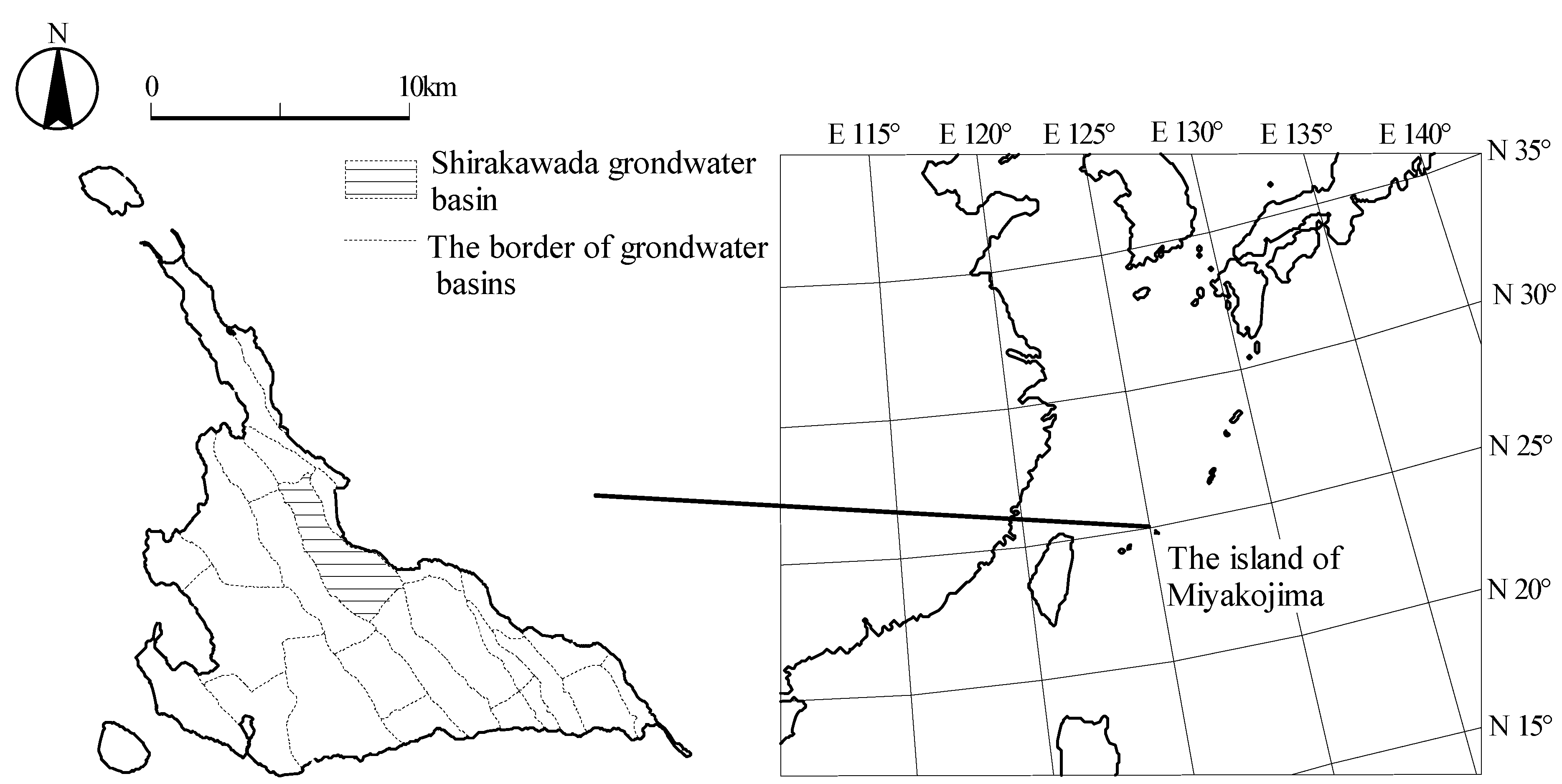
2.1. Study Site

Our study site is in a sugarcane field at Saratake in the Shirakawada groundwater basin, which is one of several fault-bounded groundwater basins on Miyakojima (Figure 1). We measured precipitation (CTK-15PC, Climatec, Inc., Tokyo, Japan), temperature (CVS-HMP-155D, Climatec, Inc., Tokyo, Japan), wind speed (CPR010C, Climatec, Inc., Tokyo, Japan), net radiation (CHF-NR01, Climatec, Inc., Tokyo, Japan), evapotranspiration (CS7500, Campbell Scientific, Logan, UT, USA and SAT-540, SONIC Co., Tokyo, Japan), and VWCs (EC5, Decagon Devices, Pullman, WA, USA). Evapotranspiration was measured by the eddy covariance method [18]. Time-domain reflectometry soil moisture sensors were installed at depths of 15, 30, 50, and 70 cm. Data were collected every 30 min. Measurement started on 29 August 2009 and ended on 31 December 2009. Cultivation started on 21 February 2009 and ended on 20 January 2010.

Figure 1. Groundwater basins on the island of Miyakojima.

Figure 1. Groundwater basins on the island of Miyakojima.

The surface soil at the study site is a Jahgaru soil (gray soil [13,19]), which extends to a depth of 120 cm at our sampling site. Jahgaru soil derived from Shimajiri-mudstone is classified as Calcaric Regosols [14]. We sampled both disturbed and undisturbed soil at depths of 15, 30, 50, 70, and 100 cm. Undisturbed soil samples were collected using a 100 cm³ soil core sampler (inside diameter 5 cm, height 5.1 cm).

We measured soil particle size distributions (%), bulk densities (g·cm⁻³), hydraulic conductivities (cm·day⁻¹), and water retention curves in the laboratory. Soil particle size distributions were obtained using sieve analysis for particle sizes greater than 75 μm and by hydrometer analysis for particle sizes smaller than 75 μm, according to Japanese Industrial Standards (JIS A1202). We measured bulk densities by using the 100 cm³ soil core sampler, hydraulic conductivities by the constant-head method, and water retention curves by the three methods shown in Table 1.

Table 1. Experimental procedures used for VWC measurements at selected soil suction ranges.

Method	Log10 [ Suction (cm) ]
	1.0		1.5		2.0		2.5		3.0		3.5		4.0		4.5			5.0
Hanging water column
Pressure plate
Psychrometer *

Note: * WP4-T, Decagon Devices, Pullman, WA, USA.

Table 1. Experimental procedures used for VWC measurements at selected soil suction ranges.

Method	Log10 [ Suction (cm) ]
	1.0		1.5		2.0		2.5		3.0		3.5		4.0		4.5			5.0
Hanging water column
Pressure plate
Psychrometer *

Note: * WP4-T, Decagon Devices, Pullman, WA, USA.

2.2. HYDRUS-1D

2.2.1. Overview of HYDRUS-1D

One-dimensional water flow in soil is described by the Richards equation as follows:

$$\frac{\partial \theta }{\partial t}=\frac{\partial }{\partial z}\left(K\frac{\partial h}{\partial z}\right)+\frac{\partial K}{\partial z}-S,$$

(1)

where θ is volumetric water content (cm³·cm⁻³), t is time (s), z is the spatial coordinate, assumed positive upward (cm), h is pressure head (cm), S is a sink term for water uptake by plant roots (cm³·cm⁻³·s⁻¹), and K is unsaturated hydraulic conductivity (cm·s⁻¹). We applied the van Genuchten-Mualem equation [10,20] (VG hereafter) to estimate the water retention curve and hydraulic conductivity of the soil by using Equations (2) and (3), respectively:

$$S_e=\frac{\theta -{\theta }_r}{{\theta }_s-{\theta }_r}={\left(1+{\left|\alpha h\right|}^n\right)}^{-m},$$

(2)

$$K\left(h\right)=K_s{S_e}^l{\left[1-S_e{\left(1-{S_e}^{\raisebox{1ex}{$1$}\!\left/ \!\raisebox{-1ex}{$m$}\right.}\right)}^m\right]}^2,$$

(3)

where θ_r is residual water content (cm³·cm⁻³), θ_s is saturated water content (cm³·cm⁻³), and S_e is normalized water content. α (cm⁻¹), n, m (= 1 − 1/n) and l (= 0.5) are empirical parameters, and K_s is saturated hydraulic conductivity (cm s⁻¹).

We simulated five soil layers (0–20, 20–40, 40–60, 60–80, and 80–120 cm) that correspond to the depth ranges of the soil samples we collected. Atmospheric conditions of daily precipitation and potential evaporation were used as upper boundary conditions. Potential transpiration was used to calculate water uptake by plant roots. The lower boundary condition was free drainage. Initial VWC was the VWC measured in the field.

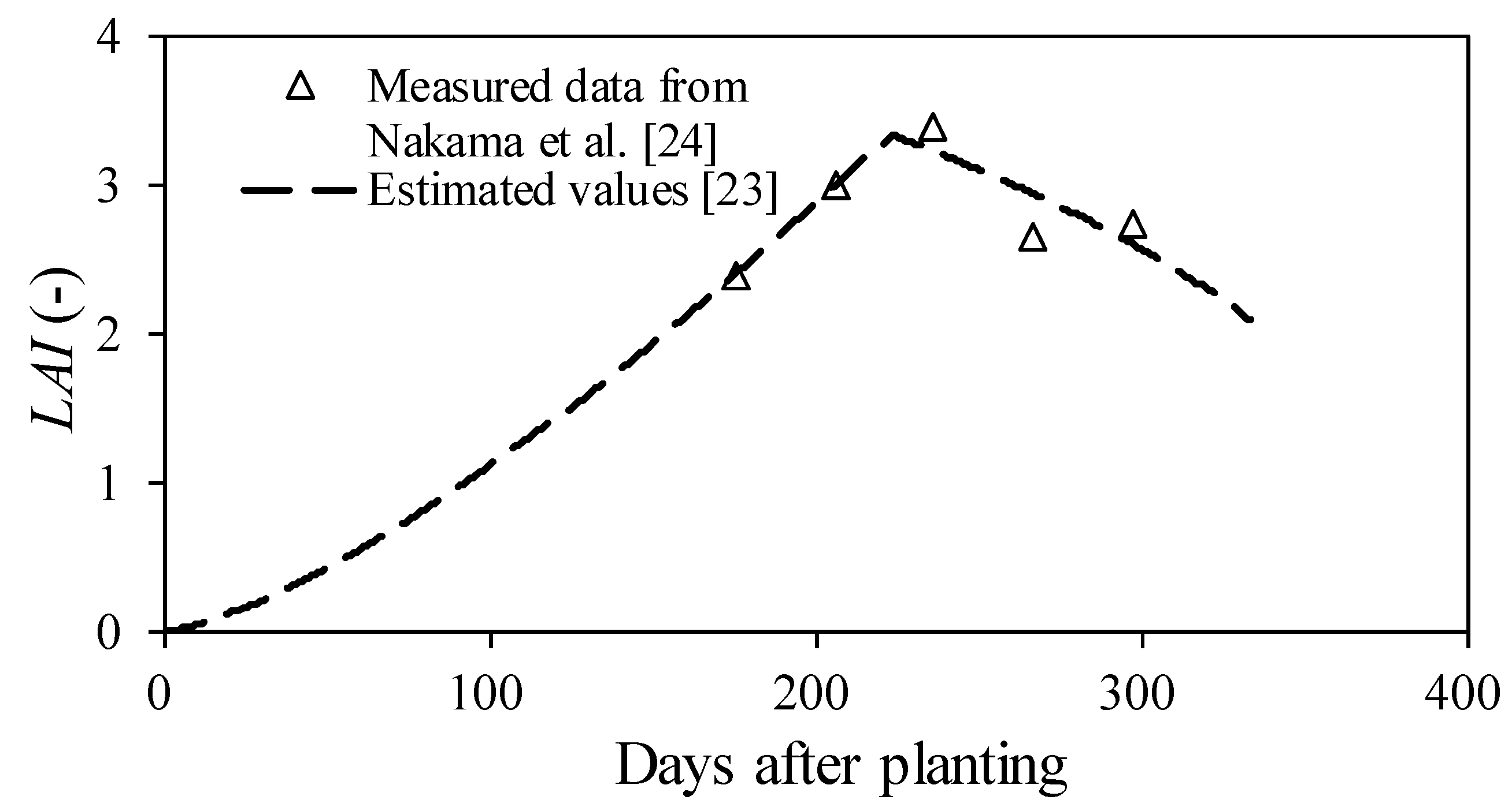
2.2.2. Crop Model in HYDRUS-1D

We used the method of van Genuchten et al. [21] to simulate water uptake by plant roots:

$$S\left(h\right)=\alpha \left(h\right)S_p,$$

(4)

$$\alpha \left(h\right)=\frac{1}{1+{\left(\frac{h}{h_{50}}\right)}^p},$$

(5)

where α(h) is the water stress response function, S_p is potential water uptake by plants roots, h₅₀ is the soil suction at which water uptake by roots is reduced by 50%, and p is an empirical component that is usually assumed to be 3 [22]. We used p = 3 to optimize h₅₀.

To determine daily root length, we used a logistic root growth function in HYDRUS-1D [2] and the results of a previous study [23]. We used the leaf area index (LAI) growth model of Larsbo and Jarvis [24]. The LAI growth model from crop emergence day (D_min) to the day of maximum LAI (D_max) is described by Equation (6), and that from D_max to the day of harvest (D_harv) by Equation (7):

$$LAI=LA{I}_{\min }+\left(LA{I}_{\max }-LA{I}_{\min }\right){\left(\frac{D^{*}-D_{\min }}{D_{\max }-D_{\min }}\right)}^{x_1},$$

(6)

$$LAI=LA{I}_{harv}+\left(LA{I}_{\max }-LA{I}_{harv}\right){\left(\frac{D_{harv}-D^{*}}{D_{harv}-D_{\max }}\right)}^{x_2},$$

(7)

where LAI_min is LAI at D_min, LAI_max is LAI at D_max, LAI_harv is LAI at D_harv, D* is the number of days after planting, and x₁ and x₂ are empirical components. We derived daily values of LAI from the results of a previous study of sugarcane [25] (Figure 2).

Potential evapotranspiration (ET_p) was calculated using the Penman equation (8) [26,27]:

$$E{T}_p=\frac{\text{Δ}}{\text{Δ}+\gamma }\cdot \frac{S}{L}+\frac{\gamma }{\text{Δ}+\gamma }\cdot u_2\left(e_{sa}-e_a\right),$$

(8)

where ET_p is the reference evapotranspiration (mm·day⁻¹), Δ is the slope of the saturation vapor pressure curve (kPa·°C⁻¹), γ is the psychometric constant (kPa·°C⁻¹), S is the net radiation (MJ·m⁻²·day⁻¹), L is the latent heat of evaporation (MJ·kg⁻¹) is, u₂ is wind speed at 2 m height (m·s⁻¹), (e_sa − e_a) is the saturation vapor pressure deficit (kPa). ET_p was partitioned into potential evaporation (E_p) and potential transpiration (T_p) using Campbell’s equation [28]:

$$T_p=E{T}_p\left[1-\exp \left(-8.2LAI\right)\right]$$

(9)

$$E_p=E{T}_p-T_p$$

(10)

Total precipitation during the observation period was 675.5 mm (Figure 3). Since the days after planting during the observation period varied from 189 to 313 and LAI from 2.4 to 3.3 (from Equations (6) and (7)), E_p was low throughout the observation period.

Figure 2. Change of LAI after planting of sugarcane.

Figure 2. Change of LAI after planting of sugarcane.

Figure 3. Daily precipitation, potential evaporation (Ep) and potential transpiration (Tp) from 29 August to 31 December 2009.

Figure 3. Daily precipitation, potential evaporation (Ep) and potential transpiration (Tp) from 29 August to 31 December 2009.

2.3. Comparison of Measured Soil Hydraulic Parameters with Those Estimated Using ROSETTA

We determined the parameters for the VG equation by using our analyses of soil samples and by application of the ROSETTA module in HYDRUS-1D. We determined VG parameters so as to minimize the difference between measured values and estimated values according to the nonlinear least-squares method using the solver of an EXCEL add-in. ROSETTA can use combinations of soil texture, particle size distribution, bulk density, and one or two points on the water retention curve to determine the parameters for the VG equation and for hydraulic conductivity. In this study, we used particle size distribution and bulk density, since these properties were readily available.

Measured particle size distribution, bulk density and hydraulic conductivity are shown in Table 2. For all samples, the sand content was less than 20% and the soil texture was silt. There were no clear differences in bulk density among soil layers. The standard deviation of hydraulic conductivity was large for all layers, which we attributed to cracks formed in response to shrinkage during drying of the soil samples. We, therefore, used the geometric mean of hydraulic conductivity in the simulations.

Table 2. Measured particle distribution, bulk density, and hydraulic conductivity of all layers.

z	Sand	Silt	Clay	Bulk Density	Saturated Conductivity, Ks
(cm)	(%)	(%)	(%)	(g·cm−3)	Geometric mean ± SD (cm·day−1)
15	13.1	69.6	17.3	1.319	24.7 ± 97.8
30	11.1	71.2	17.7	1.278	24.3 ± 152.6
50	7.5	75.3	17.2	1.268	21.8 ± 90.0
70	8.7	74.8	16.5	1.305	116.3 ± 343.8
100	10.4	70.3	19.4	1.159	21.9 ± 99.8

Note: Particle size distribution was derived from one sample and hydraulic conductivity from four samples.

Table 2. Measured particle distribution, bulk density, and hydraulic conductivity of all layers.

z	Sand	Silt	Clay	Bulk Density	Saturated Conductivity, Ks
(cm)	(%)	(%)	(%)	(g·cm−3)	Geometric mean ± SD (cm·day−1)
15	13.1	69.6	17.3	1.319	24.7 ± 97.8
30	11.1	71.2	17.7	1.278	24.3 ± 152.6
50	7.5	75.3	17.2	1.268	21.8 ± 90.0
70	8.7	74.8	16.5	1.305	116.3 ± 343.8
100	10.4	70.3	19.4	1.159	21.9 ± 99.8

Note: Particle size distribution was derived from one sample and hydraulic conductivity from four samples.

In our application of HYDRUS-1D, we considered four combinations of input soil hydraulic parameters (Cases 1 to 4; Table 3).

Table 3. Combinations of parameters input to HYDRUS-1D.

Soil Hydraulic Parameter	Case 1	Case 2	Case 3	Case 4
Retention curve	Measured	ROSETTA	ROSETTA	Measured
Hydraulic conductivity	Measured	ROSETTA	Measured	ROSETTA

Table 3. Combinations of parameters input to HYDRUS-1D.

Soil Hydraulic Parameter	Case 1	Case 2	Case 3	Case 4
Retention curve	Measured	ROSETTA	ROSETTA	Measured
Hydraulic conductivity	Measured	ROSETTA	Measured	ROSETTA

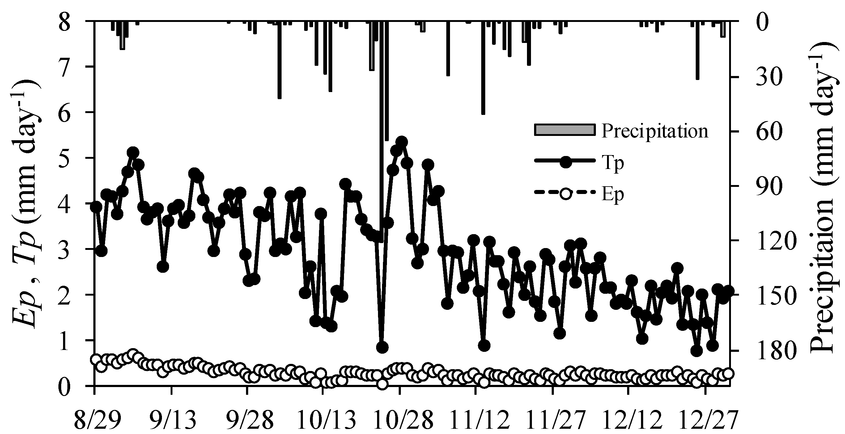
2.4. Simulation of Evapotranspiration and Volumetric Water Contents

To optimize the value of h₅₀, we needed to minimize the difference between measured and simulated evapotranspiration for each of Cases 1 to 4. To achieve this, for each case we ran HYDRUS-1D using h₅₀ values from 100 to 1000 cm at intervals of 100 cm. Then, we chose the optimum value of h₅₀ as the value with the lowest root-mean-square error (RMSE) for total evapotranspiration calculated at 10-day intervals.

To examine the influence of input soil hydraulic parameters on simulated VWCs movement, we calculated the RMSE between measured VWCs and simulated VWCs (optimized h₅₀) for each of the four soil layers for Cases 1 to 4.

3. Results and Discussion

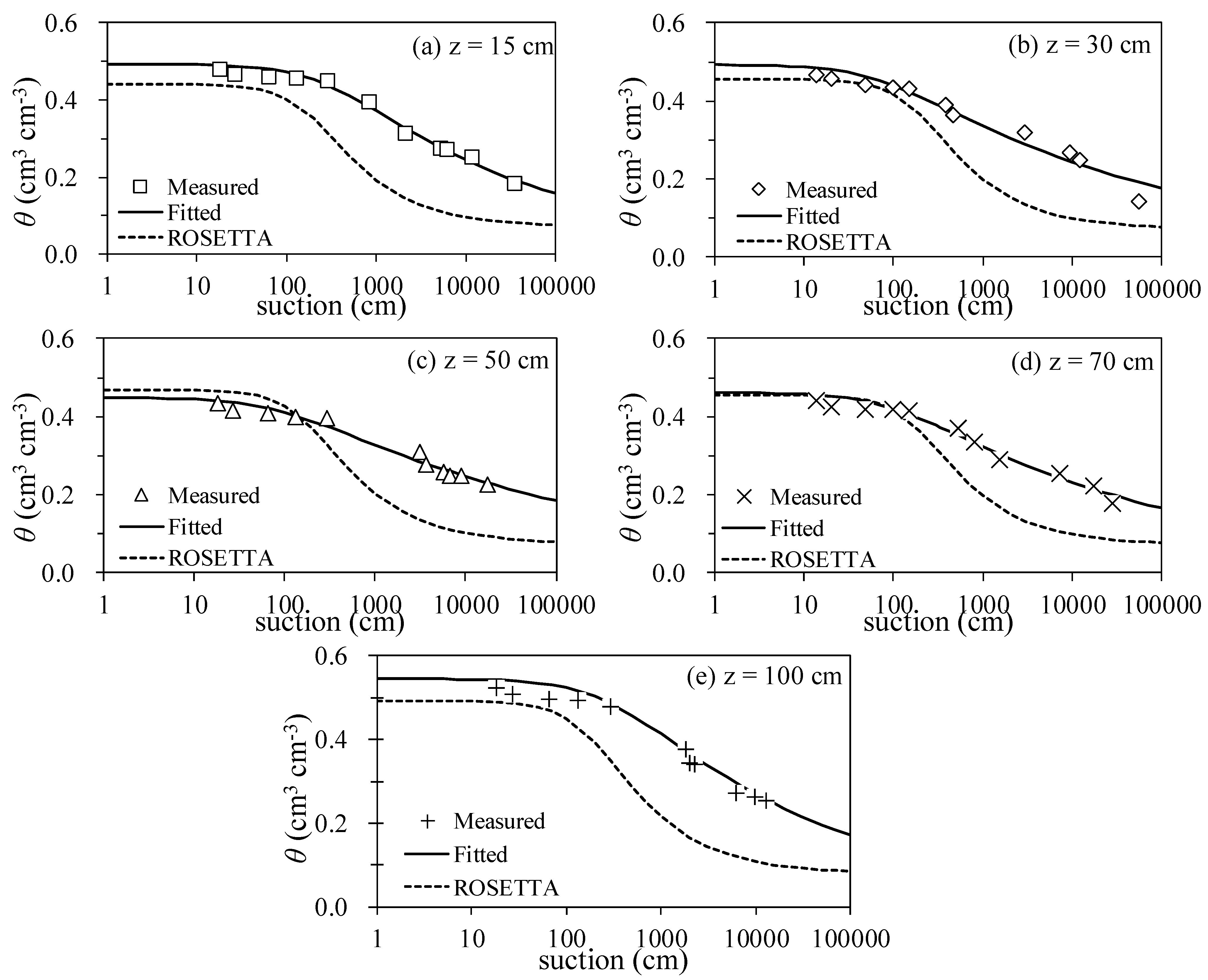
3.1. Comparison of Measured Soil Hydraulic Parameters with Those Estimated by ROSETTA

In general, ROSETTA underestimated measured VWCs, particularly for soil suctions greater than 1000 cm (Figure 4). Okamoto et al. [12] reported similar results from their application of ROSETTA to Shimajiri mahji soil. Since Jahgaru soil has a poorly developed structure [19] it often does not drain well [18]. Therefore, the measured VWC values at high suction tended to be larger than that estimated by ROSETTA (Figure 4). Schaap and Leij [29] reported that the use of PTFs to estimate soil hydraulic parameters might depend strongly on the data used for calibration. The characteristics of Jahgaru soil might be different from the soil data used to develop on the parameters used in ROSETTA.

Figure 4. Soil water retention curves from measured data and as estimated by ROSETTA. (a) z = 15 cm; (b) z = 30 cm; (c) z = 50 cm; (d) z = 70 cm; (e) z = 100 cm.

Figure 4. Soil water retention curves from measured data and as estimated by ROSETTA. (a) z = 15 cm; (b) z = 30 cm; (c) z = 50 cm; (d) z = 70 cm; (e) z = 100 cm.

Measured hydraulic conductivities were 21.8–116.3 cm d⁻¹, whereas those estimated by ROSETTA were 30.3–53.5 cm·d⁻¹ (Table 4). We attributed the difference in these results to the influence of cracks and aggregations of soil in the sugarcane field.

Table 4. Parameters used in simulations.

z (cm)	θr (cm3·cm−3)		θs (cm3·cm−3)		α (cm−1)		n		Ks (cm·d−1)
	Fitted	ROS	Fitted	ROS	Fitted	ROS	Fitted	ROS	Measured	ROS
15	0	0.070	0.493	0.441	0.0037	0.0049	1.193	1.685	24.7	30.3
30	0	0.073	0.493	0.456	0.0148	0.0049	1.140	1.683	24.3	35.0
50	0	0.074	0.449	0.469	0.0117	0.0051	1.125	1.672	21.8	35.2
70	0	0.072	0.462	0.456	0.0107	0.0050	1.147	1.677	116.3	32.3
100	0	0.078	0.556	0.492	0.0082	0.0049	1.166	1.675	21.9	53.5

Note: ROS = from ROSETTA.

Table 4. Parameters used in simulations.

z (cm)	θr (cm3·cm−3)		θs (cm3·cm−3)		α (cm−1)		n		Ks (cm·d−1)
	Fitted	ROS	Fitted	ROS	Fitted	ROS	Fitted	ROS	Measured	ROS
15	0	0.070	0.493	0.441	0.0037	0.0049	1.193	1.685	24.7	30.3
30	0	0.073	0.493	0.456	0.0148	0.0049	1.140	1.683	24.3	35.0
50	0	0.074	0.449	0.469	0.0117	0.0051	1.125	1.672	21.8	35.2
70	0	0.072	0.462	0.456	0.0107	0.0050	1.147	1.677	116.3	32.3
100	0	0.078	0.556	0.492	0.0082	0.0049	1.166	1.675	21.9	53.5

Note: ROS = from ROSETTA.

3.2. Simulation of Evapotranspiration and Volumetric Water Contents

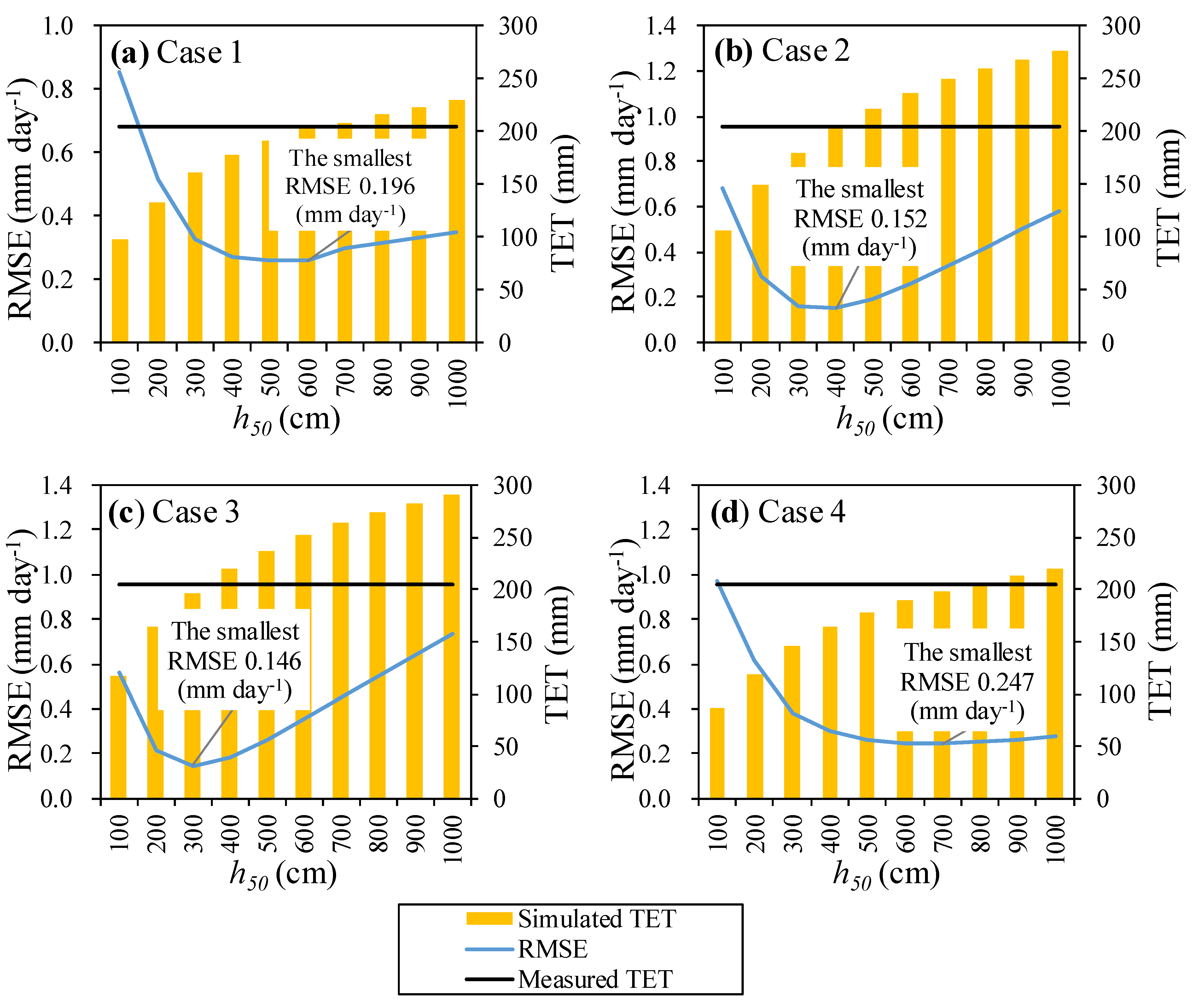
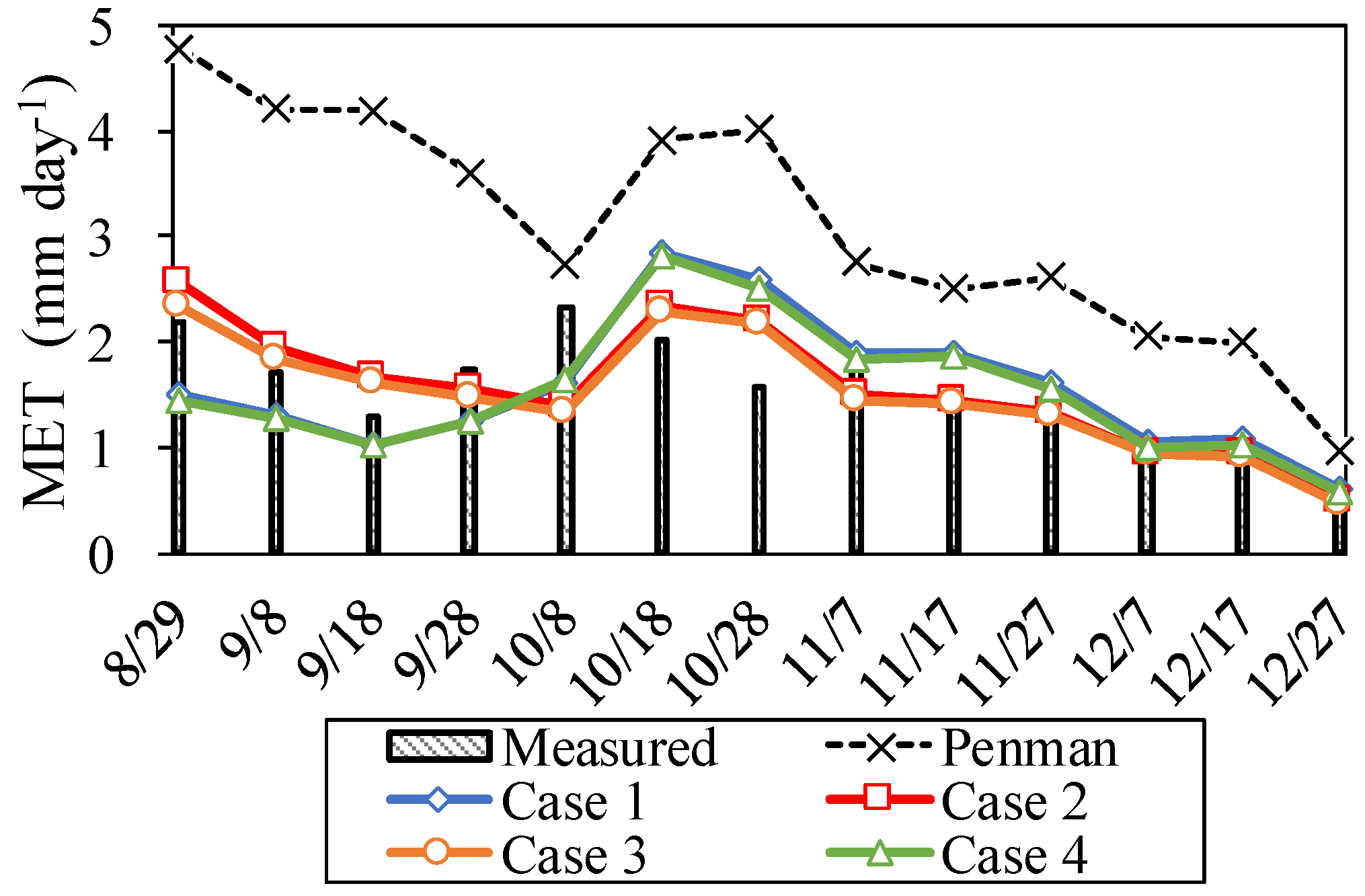
3.2.1. Optimization of h₅₀ and Simulation of Evapotranspiration

The simulations run to optimize h₅₀ (Figure 5) show that total evapotranspiration (TET) increased with increasing h₅₀ for all four cases considered. The optimal h₅₀ (smallest RMSE) was 600 cm for Case 1, 400 cm for Case 2, 300 cm for Case 3 and 700 cm for Case 4. For each of the four cases, the TET estimated with the optimized h₅₀ was almost the same as the measured TET (204.5 mm).

Figure 5. Relationships of the value of h₅₀ to RMSE and TET for each Case. (a) Case1; (b) Case 2; (c) Case 3; (d) Case 4.

Figure 5. Relationships of the value of h₅₀ to RMSE and TET for each Case. (a) Case1; (b) Case 2; (c) Case 3; (d) Case 4.

The simulation results for the pairs of cases with the same retention curve (Cases 1 and 4, Cases 2 and 3) were similar (compare Figure 5 and Figure 6). The suction required to deplete VWCs during normal growth has been reported to be about 1000 cm [30]; therefore, we considered that Case 1 (600 cm) and Case 4 (700 cm) provided the more realistic values of h₅₀ for application in HYDRUS-1D, even though the RMSEs of Cases 2 and 3 were lower. The common factor for Cases 1 and 4 was the use of the measured retention curve.

Thus, comparison of our simulation results for evapotranspiration did not clearly indicate which soil hydraulic parameters were better for application in HYDRUS-1D.

Figure 6. Comparison of simulated, measured and potential evapotranspiration at ten-day intervals (MET) from 29 August to 31 December 2009.

Figure 6. Comparison of simulated, measured and potential evapotranspiration at ten-day intervals (MET) from 29 August to 31 December 2009.

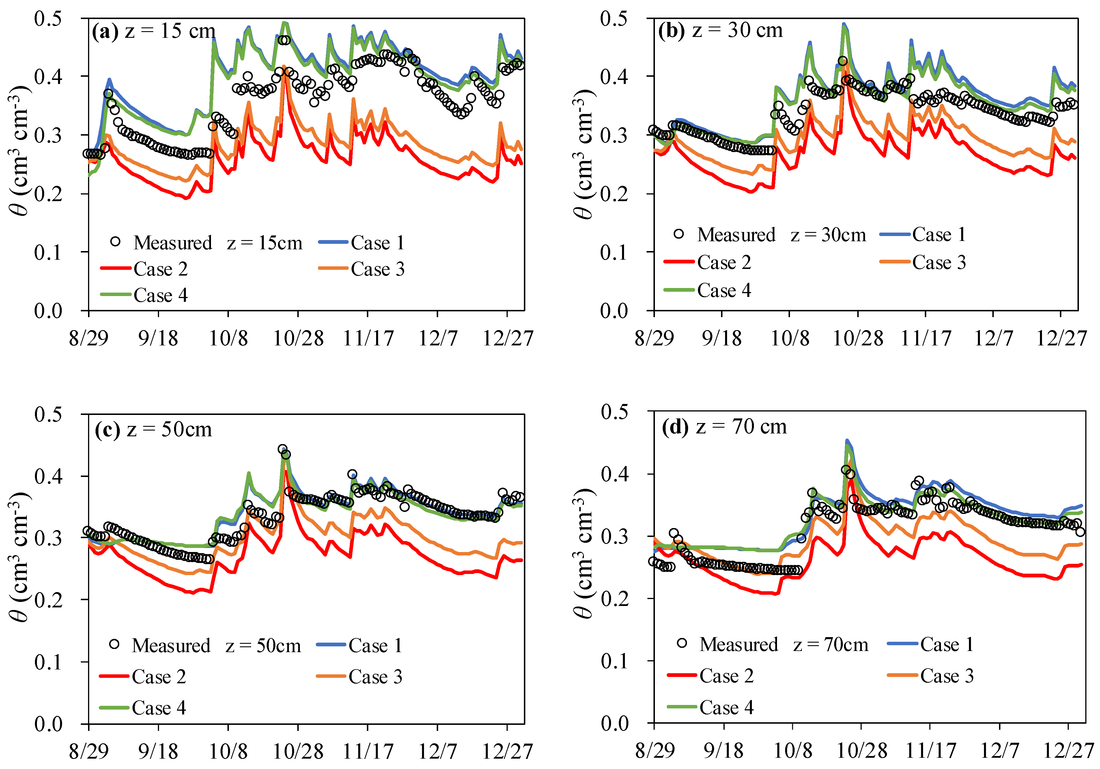
3.2.2. Influence of Soil Hydraulic Parameters on Volumetric Water Contents Simulation

The time series of simulated VWCs (Figure 7) and RMSEs between measured and simulated VWCs (Table 5) show that the simulated VWC values for Cases 2 and 3 (retention parameters estimated using ROSETTA) were lower than measured values, whereas for Cases 1 and 4 (retention parameters calculated from measured data) simulated and measured VWCs agreed well.

Figure 7. Comparison of simulated and measured daily VWCsat 4 depths from 29 August to 31 December 2009. (a) z = 15 cm; (b) z = 30 cm; (c) z = 50 cm; (d) z = 70 cm.

Figure 7. Comparison of simulated and measured daily VWCsat 4 depths from 29 August to 31 December 2009. (a) z = 15 cm; (b) z = 30 cm; (c) z = 50 cm; (d) z = 70 cm.

Table 5. RMSE between measured and simulated VWCs.

z (cm)	RMSE (cm3·cm−3)
	Case 1	Case 2	Case 3	Case 4
15	0.052	0.101	0.083	0.043
30	0.035	0.067	0.047	0.028
50	0.017	0.060	0.040	0.017
70	0.026	0.051	0.031	0.021

Table 5. RMSE between measured and simulated VWCs.

z (cm)	RMSE (cm3·cm−3)
	Case 1	Case 2	Case 3	Case 4
15	0.052	0.101	0.083	0.043
30	0.035	0.067	0.047	0.028
50	0.017	0.060	0.040	0.017
70	0.026	0.051	0.031	0.021

When considering the water budget, water recharge (Re) is calculated using

$$R_e=P-ET-\text{Δ}SW,$$

(11)

where P is precipitation, ET is evapotranspiration and ΔSW is the change of VWCs. To estimate water recharge from this equation, accurate simulations of VWCs and evapotranspiration are needed. The results of our simulations of evapotranspiration for Cases 1 to 4 (Figure 6) did not differ greatly (Section 3.2.1). However, our simulations of VWCs indicated that Cases 1 and 4 provided better results than Cases 2 and 3. These results indicate the importance of using soil hydraulic parameters based on retention curves derived from measured data to calculate the water budget for the island of Miyakojima, and likely for many or most other applications.

4. Conclusions

We drew the following main conclusions about the optimum application of HYDRUS-1D in our study area.

1)

ROSETTA software underestimated measured VWCs.

2)

Optimized values of h₅₀ were dependent on the parameters defined by the retention curve. Simulated and measured total evapotranspiration rates agreed well for all four cases considered. Since, for normal growth the amount of suction required to deplete VWCs is about 1000 cm, we consider the h₅₀ values we obtained that were closest to 1000 cm to be the more realistic. Thus, our HYDRUS-1D simulations using the measured soil hydraulic parameters provided better results than those based on parameters estimated by ROSETTA.

3)

VWCs simulated by HYDRUS-1D using parameters estimated by ROSETTA were lower than the measured values, whereas those using measured parameters agreed well with measured values.

Our study confirmed that it is important to use soil hydraulic parameters derived from measured retention data on the island of Miyakojima, rather than estimates obtained with pedotransfer function.

References

1. Climate Change and Its Impacts in Japan. Available online: https://www.env.go.jp/en/earth/cc/report_impacts.pdf (accessed on 4 September 2015).
2. Ficklin, D.L.; Luedeling, E.; Zhang, M. Sensitivity of groundwater recharge under irrigated agriculture to changes in climate, CO2 concentrations and canopy structure. Agric. Water Manag. 2010, 97. [Google Scholar] [CrossRef]
3. Leterme, B.; Mallants, D.; Jacques, D. Sensitivity of groundwater recharge using climatic analogues and HYDRUS-1D. Hydrol. Earth Syst. Sci. 2012, 16. [Google Scholar] [CrossRef]
4. Šimůnek, J.; Šejna, M.; Saito, H.; van Genuchten, M.T. The HYDRUS-1D Software Package for Simulating the One-Dimensional Movement of Water, Heat, and Multiple Solutes in Variably-Saturated Media; Department of Environmental Science, University of California Riverside: Riverside, CA, USA, 2013. [Google Scholar]
5. Zlotnik, V.A.; Wang, T.; Nieber, J.L.; Šimunek, J. Verification of numerical solutions of the Richards equation using a traveling wave solution. Adv. Water Resour. 2007, 30, 1973–1980. [Google Scholar] [CrossRef]
6. Saito, H.; Šimůnek, J.; Mohanty, B.P. Numerical analysis of coupled water, vapor, and heat transport in the vadose zone. Vadose Zone J. 2006, 5. [Google Scholar] [CrossRef]
7. Kato, C.; Nishimura, T.; Imoto, H.; Miyazaki, T. Predicting soil moisture and temperature of andisoils under a monsoon climate in Japan. Vadose Zone J. 2011, 10, 541–551. [Google Scholar] [CrossRef]
8. Stenitzer, E.; Diestel, H.; Zenker, T.; Schwartengräber, R. Assessment of capillary rise from shallow groundwater by the simulation model SIMWASER using either estimated pedotransfer functions or measured hydraulic parameters. Water Resour. Manag. 2007, 21, 1567–1584. [Google Scholar] [CrossRef]
9. Wang, T.; Zlotnik, V.A.; Šimunek, J.; Schaap, M.G. Using pedotransfer functions in vadose zone models for estimating groundwater recharge in semiarid regions. Water Resour. Res. 2009, 45. [Google Scholar] [CrossRef]
10. Van Genuchten, M.T. A closed-form equation for predicting the hydraulic conductivity of unsaturated soils. Soil Sci. Soc. Am. J. 1980, 44, 892–898. [Google Scholar] [CrossRef]
11. Wang, T.; Franz, T.E.; Zlotnik, V.A. Controls of soil hydraulic characteristics on modeling groundwater recharge under different climatic conditions. J. Hydrol. 2015, 521. [Google Scholar] [CrossRef]
12. Okamoto, K.; Sakai, K.; Cho, H.; Nakamura, S.; Nakandakari, T. Influences of a bulk density for hydraulic conductivity and water retention curve of Shimajiri maji soil, and examination of PTFs’ applicability. J. Rainwater Catchment Syst. 2015, 21, 1–6, (In Japanese with English Abstract). [Google Scholar]
13. Miyamura, N.; Iha, S.; Gima, Y.; Toyota, K. Factors limiting organic matter decomposition and the nutrient supply of soils on the Daito Ilands. Soil Microorg. 2011, 65, 119–124. [Google Scholar]
14. Classification of cultivated soils in Japan. Available online: http://soilgc.job.affrc.go.jp/Document/Classification.pdf (accessed on 4 September 2015).
15. Schaap, M.G.; Leiji, F.J.; van Genuchten, M.T. Neural network analysis for hierarchical prediction of soil water retention and saturated hydraulic conductivity. Soil Sci. Soc. Am. J. 1998, 62, 847–855. [Google Scholar] [CrossRef]
16. Schaap, M.G.; Leiji, F.J. Improved prediction of unsaturated hydraulic conductivity with the Mualem-van Genuchten model. Soil Sci. Soc. Am. J. 2000, 64, 843–851. [Google Scholar] [CrossRef]
17. Schaap, M.G.; Leiji, F.J.; Van Genuchten, M.T. Rosetta: A computer program for estimating soil hydraulic parameters with hierarchical pedotransfer function. J. Hydrol. 2001, 251, 163–176. [Google Scholar] [CrossRef]
18. Kosugi, Y.; Katsuyama, M. Evapotranspiration over a Japanese cypress forest. II. Comparison of the eddy covariance and water budget methods. J. Hydrol. 2007, 334, 305–311. [Google Scholar] [CrossRef]
19. Jayasinghe, G.Y.; Tokashiki, Y.; Kitou, M.; Kinjyo, K. Effect of synthetic soil aggregates as a soil ameliorant to enhance properties of problematic gray (“Jahgaru”) soils in Okinawa, Japan. Commun. Soil Sci. Plant Anal. 2010, 41, 649–664. [Google Scholar] [CrossRef]
20. Mualem, Y. A new model predicting the hydraulic conductivity of unsaturated porous media. Water Resour. Res. 1976, 12, 513–522. [Google Scholar] [CrossRef]
21. Van Genuchtenm, M.T. A Numerical Model for Water and Solute Movement in and Below the Root Zone; U.S. Salinity Laboratory, USDA, ARS, Riverside: CA, USA, 1987. [Google Scholar]
22. Van Genuchten, M.T.; Gupta, S.K. A reassessment of the crop tolerance response function. Indian Soc. Soil. Sci. 1993, 41, 730–737. [Google Scholar]
23. Smith, D.M.; Inman-Bamber, N.G.; Thorburn, P.J. Growth and function of the sugarcane root system. Field Crops Res. 2005, 92, 169–183. [Google Scholar] [CrossRef]
24. Larsbo, M.; Jarvis, N. MACRO 5.0: A Model of Water Flow and Solute Transport in Macroporous Soil; Department of Soil Sciences, Swedish University of Agricultural Sciences: Uppsala, Sweden, 2003. [Google Scholar]
25. Nakama, M.; Nose, A.; Miyazato, K.; Murayama, S. The Science Bulletin of the Faculty of Agriculture, University of the Ryukyus, 1st ed.; Faculty of Agriculture, University of the Ryukyus: Naha-shi, Japan, 1987; pp. 187–198. [Google Scholar]
26. Penman, H.L. Natural evaporation from open water, bare soil and grass. Proc. R. Soc. Lond. A 1948, 193, 120–145. [Google Scholar] [CrossRef]
27. Miura, T.; Okuno, R. Detailed description of calculation of potential evapotranspiration using the Penman equation. Trans. Jpn. Soc. Irrig. Drain Reclam Eng. 1993, 164, 163. [Google Scholar]
28. Campbell, G.S. Soil Physics with Basics, Transport Models for Soil-Plant Systems, 1st ed.; Elsever: New York, UN, USA, 1985; p. 144. [Google Scholar]
29. Schaap, M.G.; Leiji, F.J. Database-related accuracy and uncertainty of pedotransfer functions. Soil Sci. 1998, 163, 765–779. [Google Scholar] [CrossRef]
30. Yanagawa, A.; Fujimaki, H. Tolerance of canola to drought and salinity stresses in terms of root water uptake model parameters. J. Hydrol. Hydromech. 2013, 61, 73–80. [Google Scholar] [CrossRef]