Multi-Site Calibration of Linear Reservoir Based Geomorphologic Rainfall-Runoff Models

Abstract

Multi-site optimization of two adapted event-based geomorphologic rainfall-runoff models was presented using Non-dominated Sorting Genetic Algorithm (NSGA-II) method for the South Fork Eel River watershed, California. The first model was developed based on Unequal Cascade of Reservoirs (UECR) and the second model was presented as a modified version of Geomorphological Unit Hydrograph based on Nash’s model (GUHN). Two calibration strategies were considered as semi-lumped and semi-distributed for imposing (or unimposing) the geomorphology relations in the models. The results of models were compared with Nash’s model. Obtained results using the observed data of two stations in the multi-site optimization framework showed reasonable efficiency values in both the calibration and the verification steps. The outcomes also showed that semi-distributed calibration of the modified GUHN model slightly outperformed other models in both upstream and downstream stations during calibration. Both calibration strategies for the developed UECR model during the verification phase showed slightly better performance in the downstream station, but in the upstream station, the modified GUHN model in the semi-lumped strategy slightly outperformed the other models. The semi-lumped calibration strategy could lead to logical lag time parameters related to the basin geomorphology and may be more suitable for data-based statistical analyses of the rainfall-runoff process.

1. Introduction

An accurate simulation of the rainfall-runoff process can play a significant role in urban and environmental planning, land use, flood and water resources management of a watershed as well as mitigation of drought impacts on water resources systems. That is why numerous models have been developed to simulate this complex process. A comprehensive classification of such models has been presented by Nourani et al. [1].

A distributed model includes spatial variations in all variables and parameters, while a lumped model takes into account the average values for the entire catchment. The main property of distributed model is the spatially distributed nature of the inputs, which leads to the utilization of physically based parameters. In this case, a model may be physically based in a theory, but sometimes it may not be consistent with observations because of the mismatch of scales, in which case a dimensional analysis might be required to solve the problem. Furthermore, these fully distributed models usually have many physically based parameters, which must be defined through huge amounts of field data. Contrary to distributed models, lumped conceptual models often contain many parameters; however, these parameters cannot usually be related to physical watershed characteristics and will not, consequently, have a clear physical meaning; in addition, lumped models usually calculate the runoff hydrograph only at the watershed outlet [1]. As a result, parameters of lumped models must be estimated by a calibration process using observed data. The linear reservoir model presented by Zoch in 1934 is one of the oldest and simplest conceptual models for simulation of the rainfall–runoff relationship and constitutes the basis of many conceptual models [2]. Nash [3] proposed a conceptual model composed of a cascade of linear reservoirs with equal storage coefficients, which has been one of the most popular models since it provides an explicit equation for the Instantaneous Unit Hydrograph (IUH) of a watershed wherein reservoirs have a quasi-physical meaning. To overcome the above-mentioned problems regarding fully distributed and conceptual models, new generations of models, semi-distributed models, have been and are still being developed (e.g., [4,5]). Many of these models introduce routing on the basis of the basin geomorphology and lead to the Geomorphological Unit Hydrograph (GUH). Dooge [6] presented the cell model, which probably was the first semi-distributed model. The cascade of unequal linear reservoirs models has been discussed by Maddaus and Eaglson [7], O’Meara [8], Bravo et al. [9], and Singh and McCann [10]. Boyd [11,12] developed the watershed bounded network model to create a network representation for the synthesis of the IUH employing geomorphologic and hydrologic characteristics of the watershed. Agirre et al. [13] and López et al. [14] presented unit hydrograph models using watershed geomorphology and the linear reservoir concept with a constant calibrated lag time for all reservoirs. López et al. [15] compared the previously developed one-parameter IUH model with four other IUH models in three experimental watersheds in the north of Spain. Nourani et al. [16] developed the Geomorphological Unit Hydrograph based on Nash’s model (GUHN), the Geomorphological Unit Hydrograph based on the Cascade of linear Reservoirs (GUHCR) and the Semi-distributed Linear Reservoirs Cascade (SLRC) models and compared their results with the results of the Nash and Soil Conservation Service models. In their models, all of the geomorphological parameters were determined via Geographical Information System (GIS) tools and only one hydrological parameter of each model was calibrated using observed rainfall–runoff data sets. The SCS model did not show reliable results. Considering the model structure, Nash’s model is a fully lumped model, the GUHN model is a type of lumped model with the ability of rainfall excess distribution over each sub-basin, and the GUHCR and the SLRC models are semi-distributed models with linear and non-linear routing ability, respectively. Because of the semi-distributed routing capability of the GUHCR and SLRC models, they led to better results. However, based on average values of efficiency coefficients during calibration and verification processes, the GUHN model slightly outperformed the other models.

The estimation of parameters is an inevitable affair in every conceptual and geomorphology based rainfall–runoff model. Several studies have shown that the parameter estimation problem is nonlinear, ill posed, multimodal, and non-convex for most hydrologic applications [17,18]. The present complications lead to significant usage of a population-evolution based search strategy as a method for automatic parameter estimation. Early attempts in automatic parameter estimation focused on using a single objective fitness function. One of the common population-evolution based search methods in this regard is the Genetic Algorithms (GA) [19,20,21,22,23,24].

Some studies have illustrated the need for the presentation of a new pattern that takes into account the inherent multi-objective nature of model calibration and the important role of model uncertainties and errors [25]. In this regard, multi-objective calibration approaches become a necessity due to the development of fully or semi-distributed models to indicate multiple fluxes and spatial variabilities of information. In a multi-objective optimization problem with conflicting objectives, the Pareto optimality concept is usually an appropriate choice, originally introduced by Vilfredo Pareto in 1896 [26]. In fact, instead of finding a unique best global optimum parameter value, a set of “non-dominated” or “Pareto optimal” parameter values are obtained that represent the optimal trade-off among all the objectives [26]. Based on this concept, one dominant population-evolution based search method for multi-objective optimization, analogous to the work on single-objective field, is GA [27,28,29,30,31].

A representative classical GA application in multi-objective optimization is the Non-dominated Sorting Genetic Algorithm, NSGA-II [32]. This method uses the Goldberg [33] Pareto ranking scheme to find a Pareto-optimal set whose successful applications in rainfall-runoff modeling has been asserted by a remarkable number of studies [34,35,36].

The choice of the objective functions to be considered in the multi-objective calibration framework is based on the model duty. Madsen [37] presented the following terminologies for the specification of multi-objective calibration criteria based on three types of information:

• Multi-variable data (including river discharge, groundwater level, sediment load, etc.);
• Multi-site data (several observation sites within the river basin for the same variable);
• Multi-response modes (independent objective functions that evaluate various aspects of a single process; typically discharge).

Since any parameter estimation approach, through data-fitting, is inherently multi-objective, multi-site, multi-variable watershed modeling is becoming an important tool for evaluating watershed problems.

The reasons for the increased frequency of multi-site applications probably lie in a greater availability of measured data, sophistication, and the computational ability of the improved model; benefitting from the same advantages, the focus of the present study is on the multi-site type of multi-objective calibration.

Andersen et al. [38] and Wooldridge et al. [39], among others, emphasized the importance of considering multiple flow gages during the calibration of a semi-distributed model and indicated that using the information exclusively attained from only the catchment outlet gage revealed significant defects in parameter estimation for some tributaries in the upstream. Multi-site data have been used to calibrate parameter values in numerous hydrologic models, such as the Soil Water Assessment Tool [36,40,41,42], MIKE-SHE [38,43,44] and ModSpa [45].

The major aim of the study is a novel application of multi-site optimization scheme in the event-based rainfall-runoff modeling using linear reservoir concept. This is a way to interrelate and contribute the interior data measured at outlets of one or some sub-basins within the calibration framework. Such a calibration may lead to calibrated parameters with a higher physical interpretation and in turn, the implication of such parameters in the proposed semi-distributed model to get better flow routing results for the interior points of watershed (the outlet of sub-basins without any observed and measured data). For this purpose, three minor objectives are also considered. The first is the evaluation and comparison of two event-based hydrologic models in a multi-site framework. The second objective is to present a novel application of two calibration strategies (semi-lumped and semi-distributed) in the event-based rainfall-runoff modeling. These are two possible parameterization methods for imposing (or unimposing) the geomorphology relations in the models. Finally, the third objective is to perform a special optimization tool (NSGA-II) based on the multi-objective nature of the problem, which is different from conventional optimization methods. The two latter minor objectives, which are concurrently operated in a unique framework, are not separable and provide the needed tools to attain the ultimate aim of the research, i.e., the multi-site modeling.

This paper emphasizes on simultaneously imposing the data of two stations in the modeling whereas in most of the other studies, the emphasis of the modeling is on the watershed’s outlet behavior i.e., single site calibration is performed only with regard to the outlet data.

The proposed linear models are based on the unit hydrograph theory and implication of some IUHs like the IUH of Nash, linear reservoir, and linear channel. Therefore due to the linearity of the proposed models, they are applicable to the other watersheds due to the properties of proportionality and superposition, provided that the related parameters are calibrated for each case study.

2. Materials and Methods

2.1. Study Area and Data

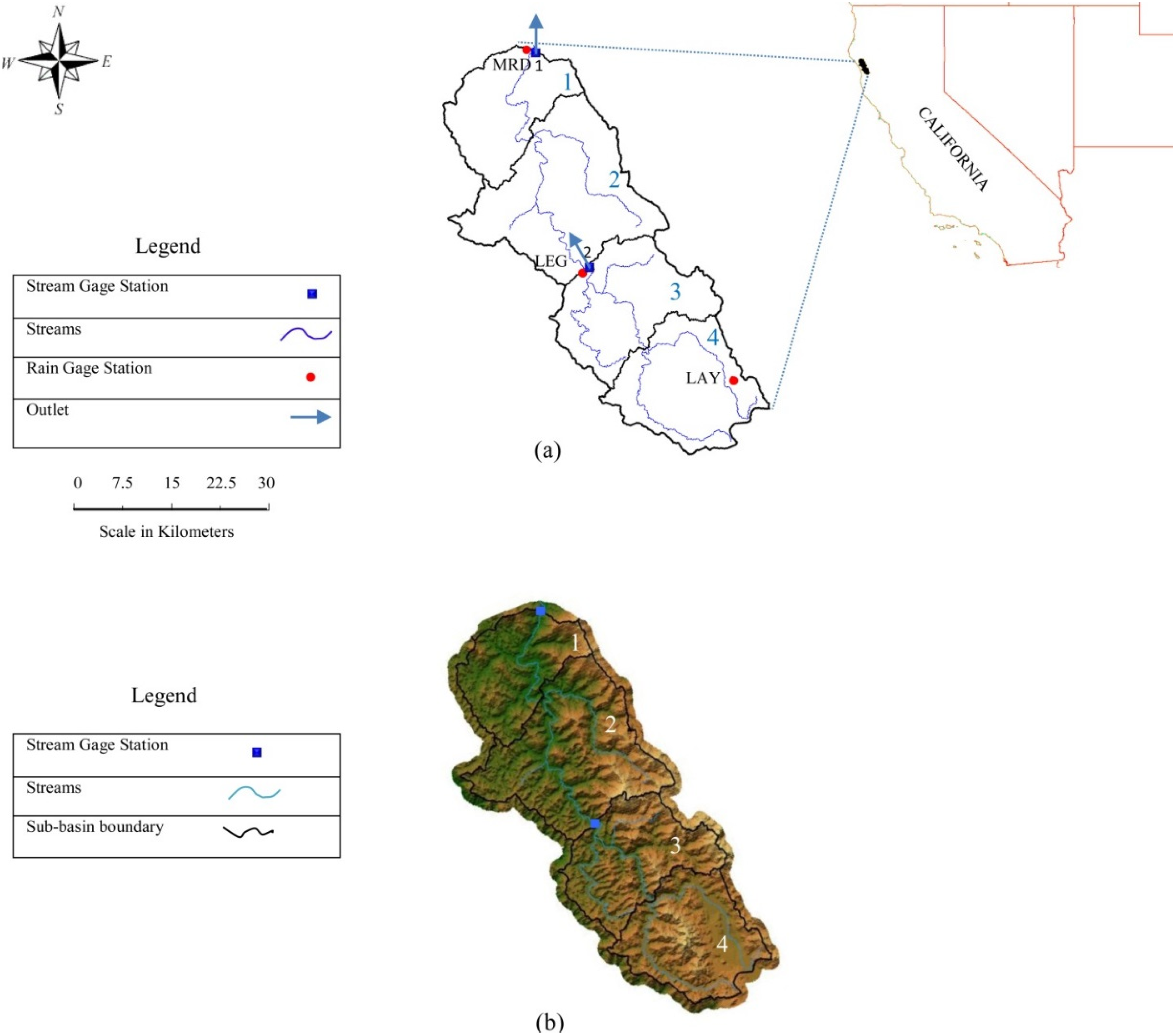
To carry out the empirical phase of the study, the South Fork Eel River watershed in California was selected. The South Fork Eel River watershed near Miranda (USGS ID = 11476500) with a drainage area of 1390.8 km² is located between 39°36'11" N and 40°10'55" N latitude and 123°25'32" W and 123°57'54" W longitude. Watershed elevation varies between 68 m and 1369 m above sea level and its longest watercourse is about 136 km long. It drains a rugged area between the Sacramento valley and the ocean, crossing the Humboldt and Mendocino counties. For most of its course, the river flows to the northwest, parallel to the coast. Figure 1 shows the map of the study area. The predominant land uses throughout the basin are timber harvest, livestock grazing, and dispersed rural development; the amount of basin covered by forest is about 51%. Rugged terrain throughout the basin is underlain by soft Franciscan geology, which combines with high winter precipitation leading to high instream sediment loads. The average daily air temperature ranges from 6 °C in January to as much as 31 °C in August and the average annual precipitation is about 178 cm. The monthly minimum temperature is about 4 °C in January and this means the South Fork Eel River watershed is a rain-dominated watershed and there is no problem from snow melt. The hourly discharge data are available for two stations located inside the watershed at the USGS website [46]. Each station was considered as an outlet for the related upstream sub-basin.

Figure 1. South Fork Eel River watershed at Miranda. (a) Situation map; (b) Geomorphological map.

Figure 1. South Fork Eel River watershed at Miranda. (a) Situation map; (b) Geomorphological map.

The information about the stations and related sub-basins are presented in Table 1. Furthermore, hourly rainfall data are available for three rain gauges (MRD, LEG, and LAY) at the California Data Exchange Center website [47]. From the recorded data in the South Fork Eel River, 18 storms, as representatives of different seasons (except summer) and rainfall depth and duration, were selected, in which 10 storms were used in the calibration step and the remaining eight storms for the verification. In event-based modeling, it is common to separate the baseflow from the total runoff hydrograph, to produce the direct runoff hydrograph. A number of methods have been proposed for separating the direct runoff and baseflow. In this study, the fixed gradient method was employed [2]. Then, the volume of direct runoff could be computed to use to separate the rainfall. The initial abstraction was identified and separated from the measured rainfall hyetograph. The remaining part of the rainfall hyetograph should then be separated into losses and rainfall excess, such that the volume of rainfall excess equals the volume of direct runoff. A number of methods have been proposed to estimate losses, and in this study, the Φ index method was used [2]. Geomorphological factors extracted by GIS to determine the model parameters, and specifications of storm events for two stream stations are illustrated in Table 1, Table 2 and Table 3, respectively.

2.2. Proposed Geomorphology-Based Models

The significance of integrating geomorphology information in the rainfall-runoff models and the determination of the model parameters using watershed geomorphologic information lies in the fact that they can lead us to apply such models for watersheds, which suffer from the lack of observations.

For this purpose, as will be presented in the Optimization procedure section, two different calibration strategies were applied to the models, namely, semi-lumped and semi-distributed. In order to impose geomorphology information in the models, semi-lumped calibration strategy was used. In this way, GIS tools used for determining geomorphological parameters of the watershed.

Recently, Nourani et al. [16] presented three geomorphology based models from which two are adapted in this study to examine the proposed multi-site calibration process: the Geomorphological Unit Hydrograph based on Nash’s Model (GUHN) and the Geomorphological Unit Hydrograph based on Cascade of linear Reservoirs (GUHCR).

Table 1. Information about stream gauge stations.

Station number	Station USGS ID	Station name	Longitude	Latitude	Drainage area (km2)
1	11476500	Miranda	123°46'30" W	40°10'55" N	1390.3
2	11475800	Leggett	123°43'10" W	39°52'29" N	642.0

Table 1. Information about stream gauge stations.

Station number	Station USGS ID	Station name	Longitude	Latitude	Drainage area (km2)
1	11476500	Miranda	123°46'30" W	40°10'55" N	1390.3
2	11475800	Leggett	123°43'10" W	39°52'29" N	642.0

Table 2. Information about sub-basins.

Sub-basin number	Sub-basin area Ai (km2)	Longest flow path length Li (m)	Overland slope Soi (%)	Stream slope Sti (%)
1	259	26,547	0.3278	0.0017
2	489.3	43,668	0.3666	0.0030
3	318.4	26,823	0.4037	0.0056
4	323.6	39,115	0.3070	0.0078

Table 2. Information about sub-basins.

Sub-basin number	Sub-basin area Ai (km2)	Longest flow path length Li (m)	Overland slope Soi (%)	Stream slope Sti (%)
1	259	26,547	0.3278	0.0017
2	489.3	43,668	0.3666	0.0030
3	318.4	26,823	0.4037	0.0056
4	323.6	39,115	0.3070	0.0078

Table 3. Characteristics of used events.

Event	Date Day/Month/Year	Total rainfall (mm)	Station No.1	Excess rainfall duration (hour)	Total rainfall (mm)	Station No.2	Excess rainfall duration (hour)
			Excess rainfall (mm)			Excess rainfall (mm)
1	28/11/2003	107.0	46.2	9	51.1	20.6	9
2	23/02/2008	79.8	26.4	20	35.0	14.5	18
3	04/05/2009	96.5	29.3	7	43.5	14.4	7
4	31/11/2009	38.2	15.5	12	11.8	3.7	3
5	12/03/2010	39.4	14.6	5	13.9	6.4	5
6	11/04/2010	39.2	9.8	20	18.4	5.5	21
7	26/04/2010	98.8	31.9	13	36.3	13.6	36
8	24/10/2010	137.7	15.5	3	48.4	8.5	4
9	28/10/2010	76.5	44.2	30	33.2	22.3	30
10	13/11/2010	45.8	16.0	4	15.0	7.6	11
11	28/11/2010	76.6	44.2	13	33.2	22.3	12
12	13/01/2011	25.3	6.7	1	6.7	3.9	4
13	15/03/2012	68.1	35.6	29	26.5	14.6	27
14	12/04/2012	54.7	15.5	35	19.1	7.2	35
15	19/01/2012	91.6	27.5	13	75.2	22	11
16	20/11/2012	50.6	7.5	2	35	6.5	16
17	4/12/2012	71.8	30.8	13	69.1	28.7	13
18	16/12/2012	30.9	16.7	5	24.4	16.1	9

Table 3. Characteristics of used events.

Event	Date Day/Month/Year	Total rainfall (mm)	Station No.1	Excess rainfall duration (hour)	Total rainfall (mm)	Station No.2	Excess rainfall duration (hour)
			Excess rainfall (mm)			Excess rainfall (mm)
1	28/11/2003	107.0	46.2	9	51.1	20.6	9
2	23/02/2008	79.8	26.4	20	35.0	14.5	18
3	04/05/2009	96.5	29.3	7	43.5	14.4	7
4	31/11/2009	38.2	15.5	12	11.8	3.7	3
5	12/03/2010	39.4	14.6	5	13.9	6.4	5
6	11/04/2010	39.2	9.8	20	18.4	5.5	21
7	26/04/2010	98.8	31.9	13	36.3	13.6	36
8	24/10/2010	137.7	15.5	3	48.4	8.5	4
9	28/10/2010	76.5	44.2	30	33.2	22.3	30
10	13/11/2010	45.8	16.0	4	15.0	7.6	11
11	28/11/2010	76.6	44.2	13	33.2	22.3	12
12	13/01/2011	25.3	6.7	1	6.7	3.9	4
13	15/03/2012	68.1	35.6	29	26.5	14.6	27
14	12/04/2012	54.7	15.5	35	19.1	7.2	35
15	19/01/2012	91.6	27.5	13	75.2	22	11
16	20/11/2012	50.6	7.5	2	35	6.5	16
17	4/12/2012	71.8	30.8	13	69.1	28.7	13
18	16/12/2012	30.9	16.7	5	24.4	16.1	9

The Nash’s IUH [3] was based on the assumption that the watershed is formed of a cascade of n equal linear reservoirs with rainfall input at the uppermost reservoir. Applying this assumption within the linear reservoir model, the Gamma distribution based on n (number of reservoirs) and k (reservoir storage coefficient) will be as follows [48,49]:

(1)

where H(t) is the IUH of the Nash’s model and Γ(n) is the Gamma function of n. The convolution integral as Equation (2) allows the computation of direct runoff Q given excess rainfall (I) and the IUH of the model (H) [2,48,49]:

(2)

in which τ is the time lag between the beginning times of rainfall excess and the unit hydrograph.

In the GUHN model, a watershed was divided into different sub-basins on the basis of approximately the equal distance lines passing through the main channel reach joints and then each sub-basin accompanied by its main channel and was represented by a cascade of linear reservoirs and a linear channel. By doing this, the adapted version of Nash’s model with distributed excess rainfall was obtained. In this model the IUH of the watershed could be expressed as [16,48]:

(3)

where, subscript i = 1, 2,…, N (N is the number of sub-basins) denotes the sub-basin number; (n_i, k_i) are parameters of Nash’s model for the ith sub-basin; T_i is the linear channel lag time; H(t) is the IUH of the watershed; D is differential operator ( ); δ is Dirac delta function; A_i is ith sub-basin area; and A is the watershed area.

Parameters (n_i, k_i, T_i) of Equation (3) were computed for every sub-basin as [16]:

(4)

(5)

where S_o was the average overland slope, and L was the longest flow path in the drainage network. These empirical relations were based on Nash’s synthetic model, which was applied to British catchments and cited in different studies [48,49,50]. T_i was computed using the conventional Manning equation [16]. It should be noted that the most downstream sub-basin (i = 1) does not need the T parameter, because its outlet is exactly the watershed outlet. The values of A, S_o and L (therefore; k_i) could be determined using GIS tools. Consequently, the GUHN model had only one unknown parameter, n, with the dimension [L^−0.1], that had to be calibrated using the observed rainfall–runoff data. This parameter was calculated using the method of moments.

2.2.1. First Proposed Model (Modified GUHN)

In this study, the modified version of GUHN was used Equations (3) and (5) along with the following relations:

(6)

(7)

where k, with the dimension [TL^−1/2], is imposed to the model instead of the constant 0.79 value (in Equation (4)). Equation (6) introduces a general form of an experimental relation (Equation (4)) which was developed for British catchments by Nash, as mentioned before. In k, the dashed sign does not indicate the mean value of k. However, it is just for this reason that the parameter k in Equation (1) has been used to represent the reservoir storage coefficient; thus, here, the new parameter k was used (Equation (6)) to avoid the confusion of the notations.

On the other hand, in order to apply the model to other watersheds, the degree of freedom of the basic version of the model was increased by the change of the constant value (0.79) of the basic model to k, so that the new model was able to determine the k value for each case study during the calibration and verification processes. In this manner, the local modeling could be changed to the global modeling.

Also, a geomorphologic relation for T_i was developed based on the general form of Manning’s equation (Equation (7)) instead of the conventional Manning’s equation, which uses cross section data and the Manning coefficient value. In Equation (7), c is a parameter that should be obtained during the calibration process; L_i is the mainstream length and S_ti is the mainstream slope. In Equations (6,7) k_i,T_i are in hours; A_i in square kilometer; L_i in meters in Equation (6) and in kilometers in Equation (7), S_oi is in percent; S_ti is in hundred percent. It should be noted that the presented empirical Equation (7) somehow has a physical base. To show this physical base, if it is assumed that the effects of roughness and hydraulic radius on velocity are the same for the whole channel length, the velocity U of flow through channel can be written as:

(8)

Equation (8) is the general form of Manning’s equation, which has already been presented in other studies [51,52].

In Equation (8), B equals in which n_m is the Manning roughness coefficient and R is the hydraulic radius. B is a constant if it is assumed that n_m and R are fixed values for the whole channel length; furthermore, the time of flow T based on a simple velocity formulation is:

(9)

Therefore, travel time T down the channel is:

(10)

This equation could be obtained through the combination of Equations (8) and (9), where x is a constant and equals 1/B, L equals the channel length and S_t is the channel slope. Hence it can be seen that Equation (7) was presented based on Equation (10) so that x was changed to c, which should be calibrated to handle the assumed simplifications. Therefore Equation (7) is a combination of the general form of Manning’s equation (Equation (8)) and the simple velocity formulation (Equation (9)).

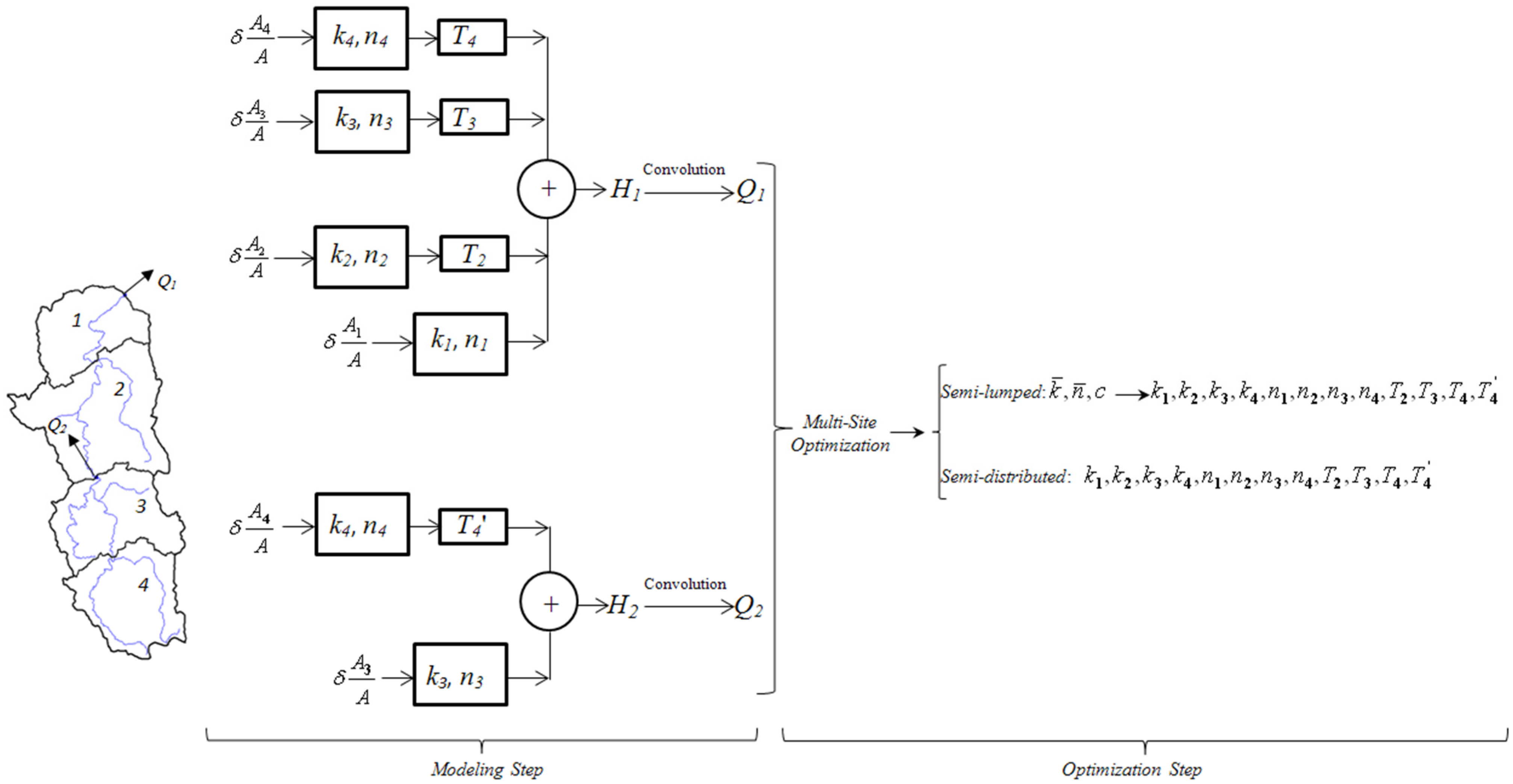
Due to the implication of the multi-site optimization framework of the available observed data in regard to the last version of the GUHN model, more degrees of freedom could be introduced to the model. Therefore, the new version of the GUHN model includes three parameters, k, n and c, that should be calibrated using the observed rainfall-runoff data. The area weighted average of recorded rainfall values in three rain gages (MRD, LEG, and LAY, Figure 1) was considered as uniform hourly rainfall over the whole watershed for simulation of runoff in Site 1 and the area weighted average of recorded values in the LEG and LAY rain gages over the related upper sub-basins was used for Site 2. The proposed schematic diagram of the new version of the GUHN model is shown in Figure 2.

In the basic version of GUHN model, the calibration process was performed for a watershed in IRAN based on eight event data just in the outlet station using the simple method of moments, but in this study, the NSGA-II method was employed for multi-site optimization of the adapted GUHN model for the South Fork Eel river watershed in California along with consideration of the semi-lumped and semi-distributed calibration strategies. For this purpose, 18 observed storms for two stations (i.e., totally 36 events) were considered, 10 storms for calibration and the remaining eight storms for the verification step.

Figure 2. Schematic diagram of modified Geomorphological Unit Hydrograph based on Nash’s model (GUHN) model.

Figure 2. Schematic diagram of modified Geomorphological Unit Hydrograph based on Nash’s model (GUHN) model.

The major differences between the modified GUHN model and the previous work [16] are the imposing the k parameter instead of the constant 0.79 (generalization of an experimental relation), applying the translation parameter T based on the general form of the Manning equation (Equation (7)) and finally determining the k, n and c parameters (applying Equations (5–7)) using the semi-lumped calibration strategy and directly determining the k_i and T_i (without applying Equations (5–7)) parameters using the semi-distributed calibration strategy. Both of the calibration strategies mentioned above were performed by the multi-site NSGA-II optimization procedure instead of the method of moments used for a single site in the previous work.

2.2.2. Second Proposed Model (Developed UECR)

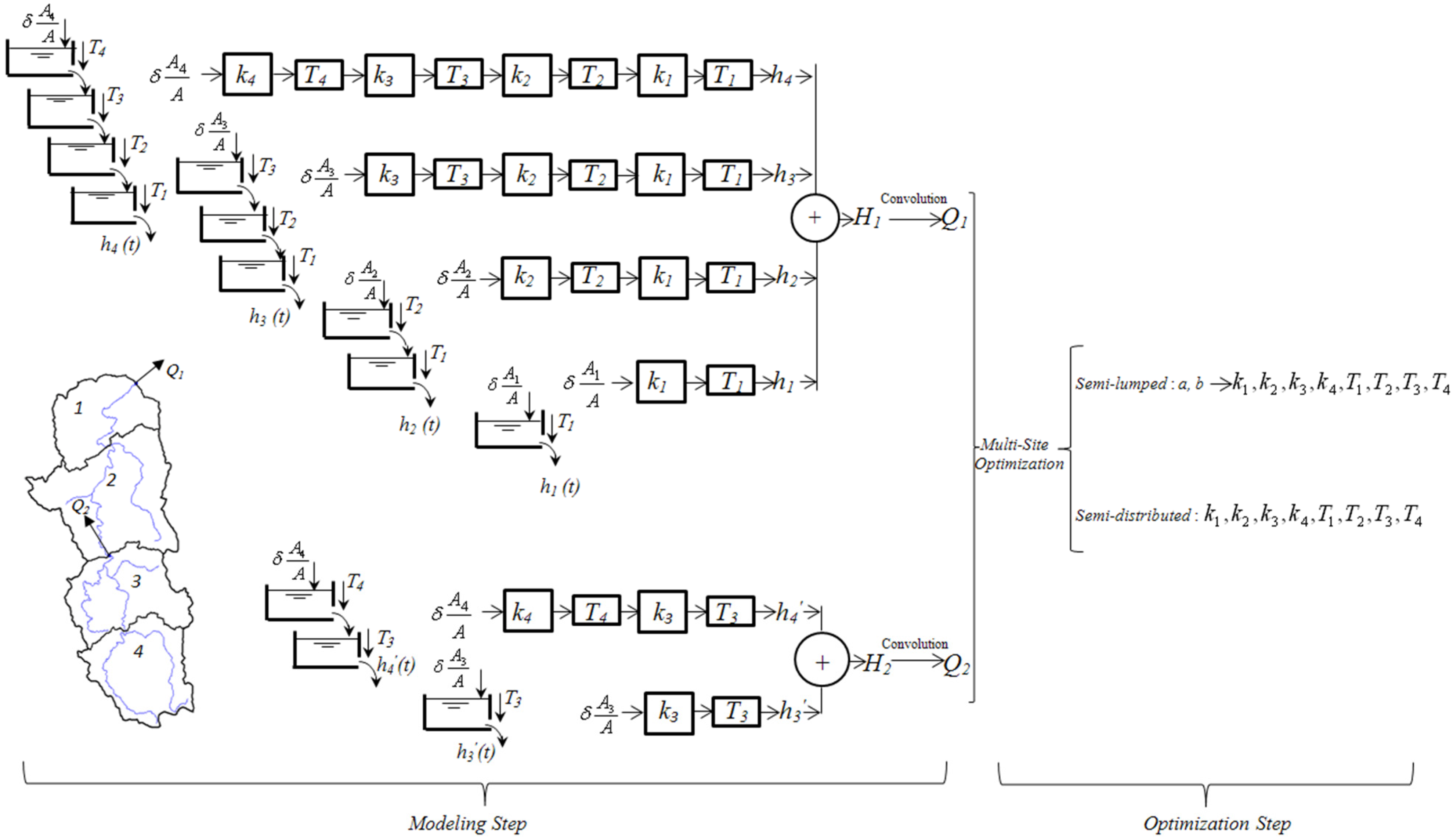
The second proposed model of this study was developed based on Unequal Cascade Reservoirs (UECR). The drainage basin was divided into several sub-basins based on the locations of the stream gage stations and the main channel reach joints (here four sub-basins), where each drainage basin was represented by a linear reservoir (Figure 3). The main excess rainfall was divided proportionally between sub-basins on the basis of their areas. To route the upstream runoff through the stream channel, a linear channel with a lag time of (T_i) was also considered for each sub-basin. It was expected that in an elongated watershed such as the South Fork Eel River, considering such parameters could lead to a better performance. The IUH of the UECR model is the same as the GUHCR model by imposing T and is expressed as [16,48]:

(11)

where T= . The h_i(t) vector in Equation (11) is a general solution for IUH and for i = N, h_N(t) = H(t) will be the watershed IUH. In the classic model of cascade of unequal linear reservoirs [48], the storage parameter (lag time) of any sub-basin (k_i), represented by a reservoir, should be determined by calibration. However, in the adopted GUHCR, k_i was related to the geomorphological properties of the sub-basin and just one unknown parameter (k, as Equation (6)) should be estimated using the observed data. In this regard the method of moments is used to determine parameter k [16].

Figure 3. Schematic diagram of developed Unequal Cascade Reservoirs (UECR) model.

Figure 3. Schematic diagram of developed Unequal Cascade Reservoirs (UECR) model.

Here, in order to incorporate the geomorphology information into the model, the linear reservoir and linear channel lag times were computed based on the sub-basins area, overland slope, main stream slope, and main stream length as:

(12)

(13)

The Equations (12) and (13) have been presented based on Equations (6) and (7). Although these relations are similar to Equations (6) and (7), it should be emphasized that the parameter values of a and b may differ from the values of k and c in the calibration process, because they are applied to two different models with different structures. It should also be noted that the operation of parameter T is slightly different in the two proposed models: this parameter is applied outside of each sub-basin to reach the whole basin outlet in the first model, but in the second model, it operates inside each sub-basin in order to reach each sub-basin’s outlet (so, L_i is computed by different methods in Equations (7) and (13)). Like in the first proposed model, multi-site NSGA-II optimization is applied as a new method in the field of linear reservoir geomorphologic based modeling.

The main differences between the UECR model and the previous work (the GUHCR model [16]) are the imposing of the new translation parameter T into the IUH formulation, relating this parameter as described by Equation (13), obtaining the a and b parameters (by applying Equations (12) and (13)) using the semi-lumped calibration strategy, and finally directly obtaining the k_i and T_i parameters (without applying Equations (12) and (13)) using the semi-distributed calibration strategy. These calibration strategies were performed by the multi-site NSGA-II optimization procedure instead of the simple method of moments applied for a single station in the previous work. A schematic diagram of the model is shown in Figure 3.

2.3. Optimization Procedure

The multi-objective nature of any parameter estimation method using data fitting necessitates the employment of the multi-site, multi-variable watershed modeling. The objective of this study was to apply the multi-objective NSGA-II optimization in a multi-site framework to the developed UECR, modified GUHN, and classic Nash models. In this study, two different calibration strategies were considered based on the spatial allocation of rainfall input and calibration parameters to each sub-basin or the whole of the basin. In the lumped calibration strategy, rainfall is averaged over the entire basin, and the calibration parameters are considered the same for the whole basin. Calibration parameters among all sub-basins are identical in the semi-lumped strategy, but are different in the semi-distributed calibration strategy; however, spatially distributed rainfall is averaged over each sub-basin in both strategies. Here, the semi-lumped calibration strategy of the proposed models was applied considering the geomorphological relations. On the other hand, the semi-distributed calibration strategy was obtained by the calibration of all conceptual parameters to have a spatial distribution of the parameters within the basin. Table 4 shows calibration strategies reported by Ajami et al. [53], but instead of physical parameters, conceptual parameters herein were used as calibration parameters.

A multi-objective search problem uses the Pareto optimality concept when the criteria are conflicting. In this way, a set of “Pareto optimal” or “non-dominated” solutions, rather than a unique optimal solution, are produced.

Pareto optimality and dominance concept briefly state that a decision variable X^* is defined as Pareto optimal when all other feasible solutions X are such that f_i(X^*) ≤ f_i(X) for all i = 1, 2, ..., n and f_i(X) < f_i(X^*) for at least one i, where n is the number of total objectives and f_i is the value of a specific objective function. This concept states that X^* is Pareto optimal if there is no feasible solution that would improve some objectives without a simultaneous degradation of performance in at least one other objective. Feasible vector solution is called Pareto set, Pareto optimal set or non-dominated set. The mapping of Pareto set from the decision space to the objective space is known as Pareto front (PF^*).

There are two approaches that can be used to solve the multi-objective optimization procedure. The first approach is to accumulate multiple objectives to a single objective framework and then one optimizer, like simple GA, is used to optimize the single objective function to find the optimal parameter values in the calibration phase. Although this method is convergent and easy to use, it has some serious problems. The considerable disadvantage of this approach is its inability to obtain multiple Pareto-optimal solutions in a single simulation run. Changing of the weights can produce various Pareto-optimal solutions, and for most large-scale watershed problems it can be computationally inefficient. Among other drawbacks, one may refer to its subjectivity in choosing weights and the infeasibility in the non-convex Pareto fronts.

Table 4. Schematics of three different calibration strategies (adapted from Ajami et al. [53]).

Calibration strategies (θ:Parameter set)
Model	Lumped		Semi-Lumped		Semi-Distributed
Modified GUHN				θ = (n, k, c)		θi = (ni, ki, Ti)
				θ1 = θ2 = θ3 = θ4		θ1 ≠ θ2 ≠ θ3 ≠ θ4
Developed UECR				θ = (a, b)		θi = (ki, Ti)
				θ1 = θ2 = θ3 = θ4		θ1 ≠ θ2 ≠ θ3 ≠ θ4
Nash

Table 4. Schematics of three different calibration strategies (adapted from Ajami et al. [53]).

Calibration strategies (θ:Parameter set)
Model	Lumped		Semi-Lumped		Semi-Distributed
Modified GUHN				θ = (n, k, c)		θi = (ni, ki, Ti)
				θ1 = θ2 = θ3 = θ4		θ1 ≠ θ2 ≠ θ3 ≠ θ4
Developed UECR				θ = (a, b)		θi = (ki, Ti)
				θ1 = θ2 = θ3 = θ4		θ1 ≠ θ2 ≠ θ3 ≠ θ4
Nash

The second approach is the Multi-Objective Evolutionary Algorithms (MOEA), as a more efficient alternative to determining simultaneous multiple Pareto-optimal solutions in one single simulation run.

For the problem presented herein, a variant of Non-dominated Sorting Genetic Algorithm, NSGA-II [32] was used as an optimizer to find the best-compromised set of parameter values in the calibration phase. Its procedure includes the appointment of dummy fitness functions based on the Pareto ranking scheme and fitness sharing, which enables maintaining a diverse set of elite population and avoids convergence to single solutions [54]. NSGA-II is started by a random generation of the parent population, P₀ with size N_ap. The parent population is sorted into different non-domination levels and for each solution a fitness value equal to its non-domination level, is assigned (one is the best level). Using binary tournament selection, recombination, and mutation operators, an offspring population with size N_p is created. The following steps describe the procedure [36]:

• Combine parent P_t and offspring Q_t populations to create R_t with size 2 N_p.
• Perform non-dominated sorting to R_t and identify different fronts F_i, i = 1, 2, ..., m and stop here if convergence criteria have been met.
• P_t+1 with size N_p is created by choosing solutions from subsequent non-dominated fronts (F₁, F₂, ..., F_m).
• Create offspring population Q_t+1 of size N_p using binary tournament selection based on crowding-comparison operator, crossover and mutation performed on P_t+1.
• Repeat steps i through iv until convergence criteria are reached.

An elitist GA always favors individuals with better fitness value (rank), whereas a controlled elitist GA also favors individuals that can increase the diversity of the population even if they have a lower fitness value. It is very important to maintain the diversity of population for convergence to an optimal Pareto front. This is done by controlling the elite members of the population as the algorithm progresses. In this study, Matlab software [55] was used to perform NSGA-II algorithm. Two options in this software, namely, 'Pareto Fraction' and 'Distance Function' were used to control the elitism, where the Pareto fraction option limits the number of individuals on the Pareto front (elite members) and the distance function helps to maintain diversity on a front by favoring individuals that are relatively far away on the front.

Obviously, the Pareto set obtained on the basis of a specific data is not unique, however, within real world practical problems, there is usually a need to determine a single solution (best-compromise) from the Pareto set; therefore, detection of a unique parameter set for practical purposes remains a challenging task. The existence of extra information and hydrological experience play key roles in solving this problem.

2.4. Performance Criteria

A large number of studies have indicated that the calibration process will have to be faced successfully if the proper objective function is selected as a performance measure [25]. In assessing the performance of the proposed models, the Nash and Sutcliffe index (E) [56] between observed and calculated discharge values was used in this study as:

(14)

where Q_i,obs is the observed discharge at t = i; Q_i,sim is the simulated discharge at t = i; Q_obs is the average observed discharge and No is the number of observed data. It should be noted that Q_i,sim is the output of the model and calculated using Equation (2).

Therefore, Equation (14) was used to identify objective functions of multi-site calibration process as:

Objective1 = 1 − E₁

(15)

Objective2 = 1 − E₂

(16)

The Objectives 1 and 2 are related to Station 1 and Station 2, respectively.

The E₁ value was computed based on the difference between the computed outflow from watershed and the observed outflow; the E₂ value was computed based on the difference between the computed outflow from gage station number 2 and observed outflow at that gage station.

After performing the NSGA-II optimization, the related Pareto front in the (1 − E₁) vs. (1 − E₂) space was obtained. There are different methods to obtain the best compromise solution among other solutions of Pareto front. Therefore, in order to select a unique parameter set between other sets of Pareto front, the normalized runoff volume difference (NRVD) between the observed and the simulated streamflow was also used as:

(17)

where V_obs is the observed runoff volume and V_sim is the simulated runoff volume. Considering the direct runoff hydrograph (DRH), the runoff volume value is the area under the hydrograph’s curve (both observed and simulated).

Here, for each point in the Pareto front, the normalized runoff volume difference was computed based on the observed and simulated runoff volumes in Station 1 (Equation (17)). Station 1 or the watershed’s outlet was selected for satisfaction of overall continuity equilibrium over the whole of the watershed, so that with obtaining the minimum value of NRVD₁, the best point on the Pareto front which satisfies volume equilibrium between observed and simulated runoffs was identified. Therefore, this objective function was used for the selection of the best point on the Pareto front, and it exactly measures the error between observed and simulated runoff volumes but it works outside the NSGA-II optimization framework.

3. Calibration and Verification Results

In the first step, the multi-site calibration of the two proposed models using the NSGA-II optimization method was performed based on the two different calibration strategies; second the verification results were obtained. The results were also compared to a benchmark and simple model i.e., the Nash’s model. Comparisons between different aspects of the modeling according to the research questions are presented in the Discussion Section.

For the two-site optimization procedure, 18 simultaneous storm events observed in two stations were used, 10 events for models calibration and the remaining eight events for verification purposes (Table 3). For the above-mentioned 10 events, the calibrated parameters of the modified GUHN model with semi-lumped calibration strategy (n, k, c) along with the computed lag time parameters (using calibrated parameters of n, k, c and Equations (5–7)) and semi-distributed calibration strategy (k₁, k₂, k₃, k₄, n₁, n₂, n₃, n₄, T₂, T₃, T₄, T₄') are averaged and illustrated in Table 5. The averaged calibrated parameters of the developed UECR model via semi-lumped calibration strategy (a, b) in addition to the computed lag time parameters (using Equations (12,13)) and semi-distributed calibration strategy (k₁, k₂, k₃, k₄, T₁, T₂, T₃, T₄) are also shown in Table 5. Finally, according to the same policy the averaged calibrated parameters of the Nash’s model (n₁, k₁ for the whole watershed and n₂, k₂ for the upstream sub-basin of Station 2) are given in Table 5. Thereafter, the models were verified by the remaining eight event data using the average values of parameters obtained in the calibration phase; the obtained results of verification are tabulated in Table 6. Also, some observed vs. computed hydrographs in calibration and verification steps are shown in Figure 4 and Figure 5, respectively.

Table 5. Calibrated model parameters for different models.

Model	Parameters used in different models
GUHN semi-lumped	k	n	c	k1	k2	k3	k4	n1	n2	n3	n4	T2	T3	T4	T4'	NRVD1	NRVD2	E1	E2
Avg.	3.66	0.727	0.064	9.781	10.893	9.768	10.261	2.01	2.11	2.01	2.09	4.141	9.268	11.573	2.305	0.0135	0.0670	0.92	0.91
GUHN semi-distributed	-	-	-	k1	k2	k3	k4	n1	n2	n3	n4	T2	T3	T4	T4'	NRVD1	NRVD2	E1	E2
Avg.	-	-	-	5.771	9.55	8.077	6.571	2.74	2.97	3.32	2.09	6.844	8.758	9.286	5.142	0.0244	0.06790	0.98	0.96
UECR semi-lumped	a	-	b	k1	k2	k3	k4	-	-	-	-	T1	T2	T3	T4	NRVD1	NRVD2	E1	E2
Avg.	3.47	-	0.027	9.262	10.315	9.249	9.716	-	-	-	-	1.767	2.188	0.983	1.215	0.0889	0.1612	0.89	0.89
UECR semi-distributed	-	-	-	k1	k2	k3	k4	-	-	-	-	T1	T2	T3	T4	NRVD1	NRVD2	E1	E2
Avg.	-	-	-	9.418	7.597	10.16	10.518	-	-	-	-	2.958	2.740	0.556	0.574	0.0759	0.1123	0.92	0.92
NASH	-	-	-	k1	k2	-	-	n1	n2	-	-	-	-	-	-	NRVD1	NRVD2	E1	E2
Avg.	-	-	-	10.62	9.484	-	-	2.94	2.56	-	-	-	-	-	-	0.01450	0.07850	0.95	0.91

Table 5. Calibrated model parameters for different models.

Model	Parameters used in different models
GUHN semi-lumped	k	n	c	k1	k2	k3	k4	n1	n2	n3	n4	T2	T3	T4	T4'	NRVD1	NRVD2	E1	E2
Avg.	3.66	0.727	0.064	9.781	10.893	9.768	10.261	2.01	2.11	2.01	2.09	4.141	9.268	11.573	2.305	0.0135	0.0670	0.92	0.91
GUHN semi-distributed	-	-	-	k1	k2	k3	k4	n1	n2	n3	n4	T2	T3	T4	T4'	NRVD1	NRVD2	E1	E2
Avg.	-	-	-	5.771	9.55	8.077	6.571	2.74	2.97	3.32	2.09	6.844	8.758	9.286	5.142	0.0244	0.06790	0.98	0.96
UECR semi-lumped	a	-	b	k1	k2	k3	k4	-	-	-	-	T1	T2	T3	T4	NRVD1	NRVD2	E1	E2
Avg.	3.47	-	0.027	9.262	10.315	9.249	9.716	-	-	-	-	1.767	2.188	0.983	1.215	0.0889	0.1612	0.89	0.89
UECR semi-distributed	-	-	-	k1	k2	k3	k4	-	-	-	-	T1	T2	T3	T4	NRVD1	NRVD2	E1	E2
Avg.	-	-	-	9.418	7.597	10.16	10.518	-	-	-	-	2.958	2.740	0.556	0.574	0.0759	0.1123	0.92	0.92
NASH	-	-	-	k1	k2	-	-	n1	n2	-	-	-	-	-	-	NRVD1	NRVD2	E1	E2
Avg.	-	-	-	10.62	9.484	-	-	2.94	2.56	-	-	-	-	-	-	0.01450	0.07850	0.95	0.91

Table 6. Verification results of modified GUHN, developed UECR and Nash models.

Event	Modified GUHN model				Developed UECR model				Nash model
	Semi-lumped		Semi-distributed		Semi-lumped		Semi-distributed
	E1	E2	E1	E2	E1	E2	E1	E2	E1	E2
2	0.91	0.79	0.92	0.86	0.96	0.80	0.97	0.83	0.95	0.90
4	0.80	0.86	0.75	0.80	0.82	0.54	0.84	0.53	0.78	0.39
8	0.84	0.76	0.81	0.69	0.69	0.77	0.74	0.76	0.70	0.61
14	0.77	0.81	0.77	0.83	0.88	0.72	0.84	0.77	0.89	0.86
15	0.83	0.83	0.78	0.73	0.86	0.88	0.86	0.90	0.82	0.72
16	0.87	0.91	0.89	0.84	0.905	0.76	0.90	0.785	0.98	0.97
17	0.81	0.94	0.75	0.86	0.79	0.92	0.82	0.93	0.74	0.86
18	0.90	0.87	0.87	0.70	0.88	0.84	0.91	0.84	0.86	0.74
Avg.	0.84	0.84	0.82	0.79	0.85	0.78	0.86	0.79	0.84	0.76

Notes: E₁, E₂ = Nash and Sutcliffe indexes (or Efficiency coefficients) in stations 1 and 2, respectively.

Table 6. Verification results of modified GUHN, developed UECR and Nash models.

Event	Modified GUHN model				Developed UECR model				Nash model
	Semi-lumped		Semi-distributed		Semi-lumped		Semi-distributed
	E1	E2	E1	E2	E1	E2	E1	E2	E1	E2
2	0.91	0.79	0.92	0.86	0.96	0.80	0.97	0.83	0.95	0.90
4	0.80	0.86	0.75	0.80	0.82	0.54	0.84	0.53	0.78	0.39
8	0.84	0.76	0.81	0.69	0.69	0.77	0.74	0.76	0.70	0.61
14	0.77	0.81	0.77	0.83	0.88	0.72	0.84	0.77	0.89	0.86
15	0.83	0.83	0.78	0.73	0.86	0.88	0.86	0.90	0.82	0.72
16	0.87	0.91	0.89	0.84	0.905	0.76	0.90	0.785	0.98	0.97
17	0.81	0.94	0.75	0.86	0.79	0.92	0.82	0.93	0.74	0.86
18	0.90	0.87	0.87	0.70	0.88	0.84	0.91	0.84	0.86	0.74
Avg.	0.84	0.84	0.82	0.79	0.85	0.78	0.86	0.79	0.84	0.76

Notes: E₁, E₂ = Nash and Sutcliffe indexes (or Efficiency coefficients) in stations 1 and 2, respectively.

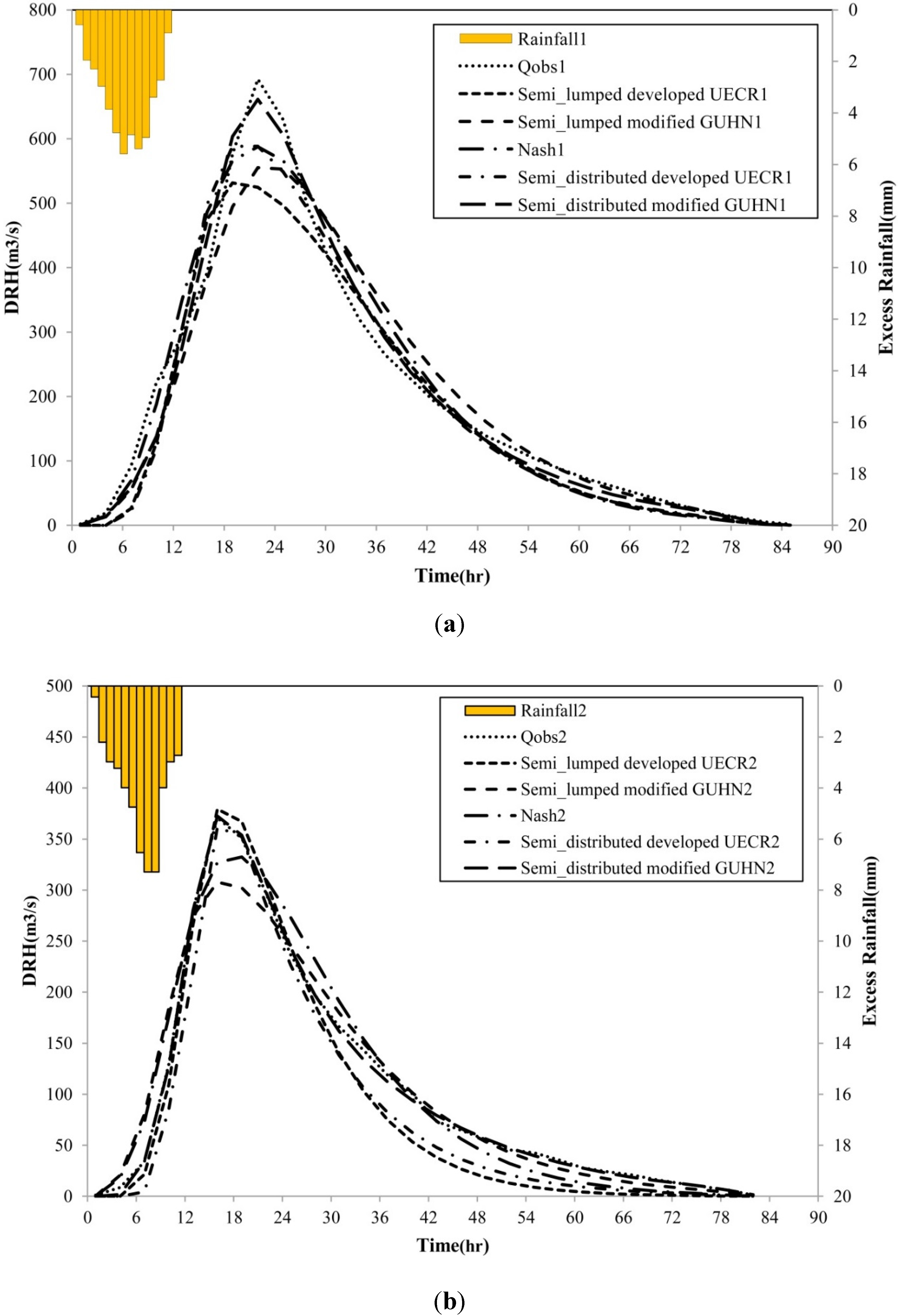
Figure 4. Calibration graphs of Nash, modified GUHN and developed UECR models. (a) Event 28 November 2010 at Outlet 1; (b) Event 28 November 2010 at Outlet 2.

Figure 4. Calibration graphs of Nash, modified GUHN and developed UECR models. (a) Event 28 November 2010 at Outlet 1; (b) Event 28 November 2010 at Outlet 2.

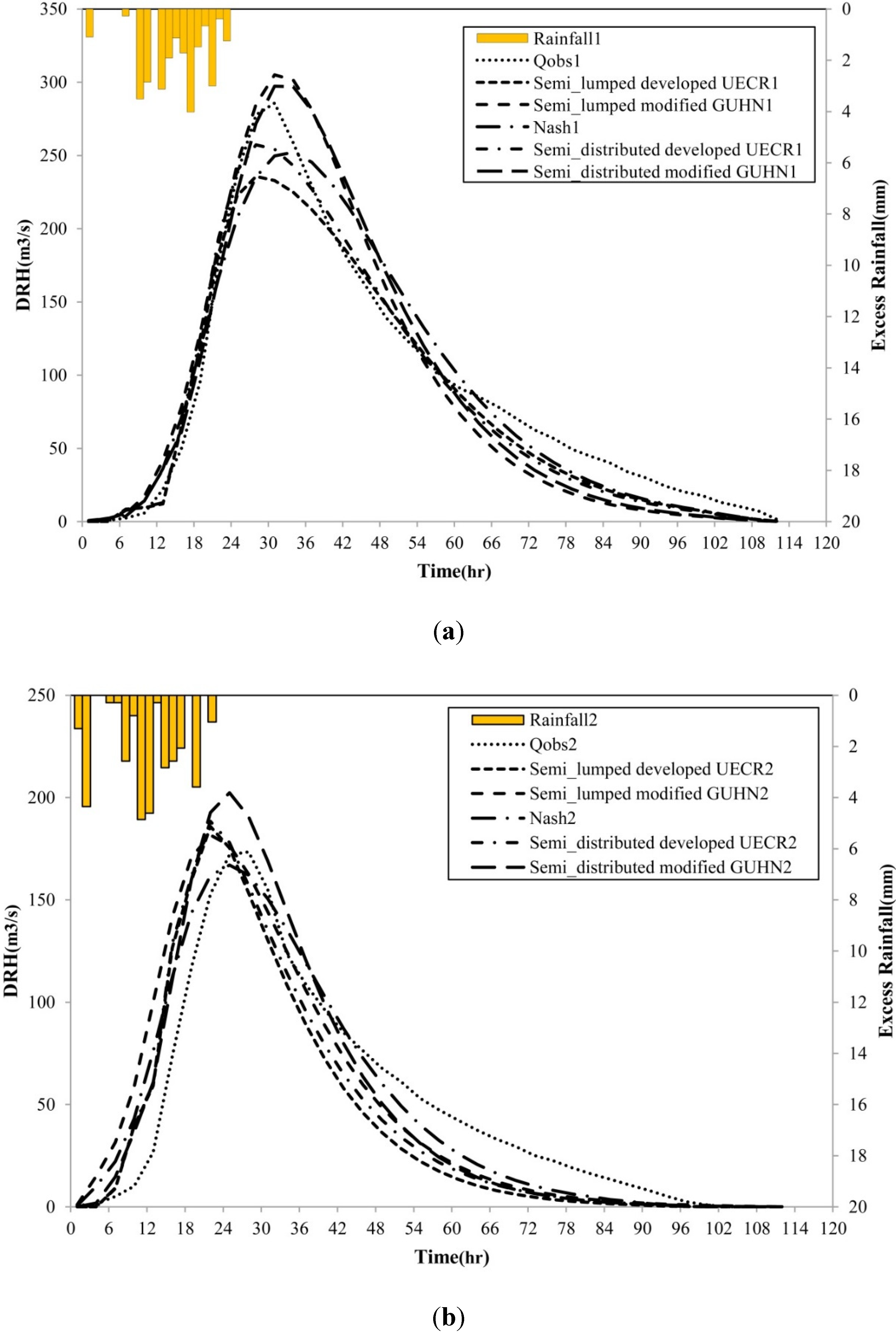
Figure 5. Verification graphs of Nash, modified GUHN and developed UECR models. (a) Event 23 February 2008 at Outlet 1; (b) Event 23 February 2008 at Outlet 2.

Figure 5. Verification graphs of Nash, modified GUHN and developed UECR models. (a) Event 23 February 2008 at Outlet 1; (b) Event 23 February 2008 at Outlet 2.

4. Discussion

In order to obtain the best compromise solution among other Pareto front solutions, experience or extra criteria such as peak discharge, time to peak discharge or runoff volume might be compared with the observed values. Owing to the importance of the runoff volume amount, the satisfaction of the continuity equation was used to find the minimum normalized runoff volume difference (NRVD) between the observed and the computed hydrographs at the watershed outlet (Equation (17)).

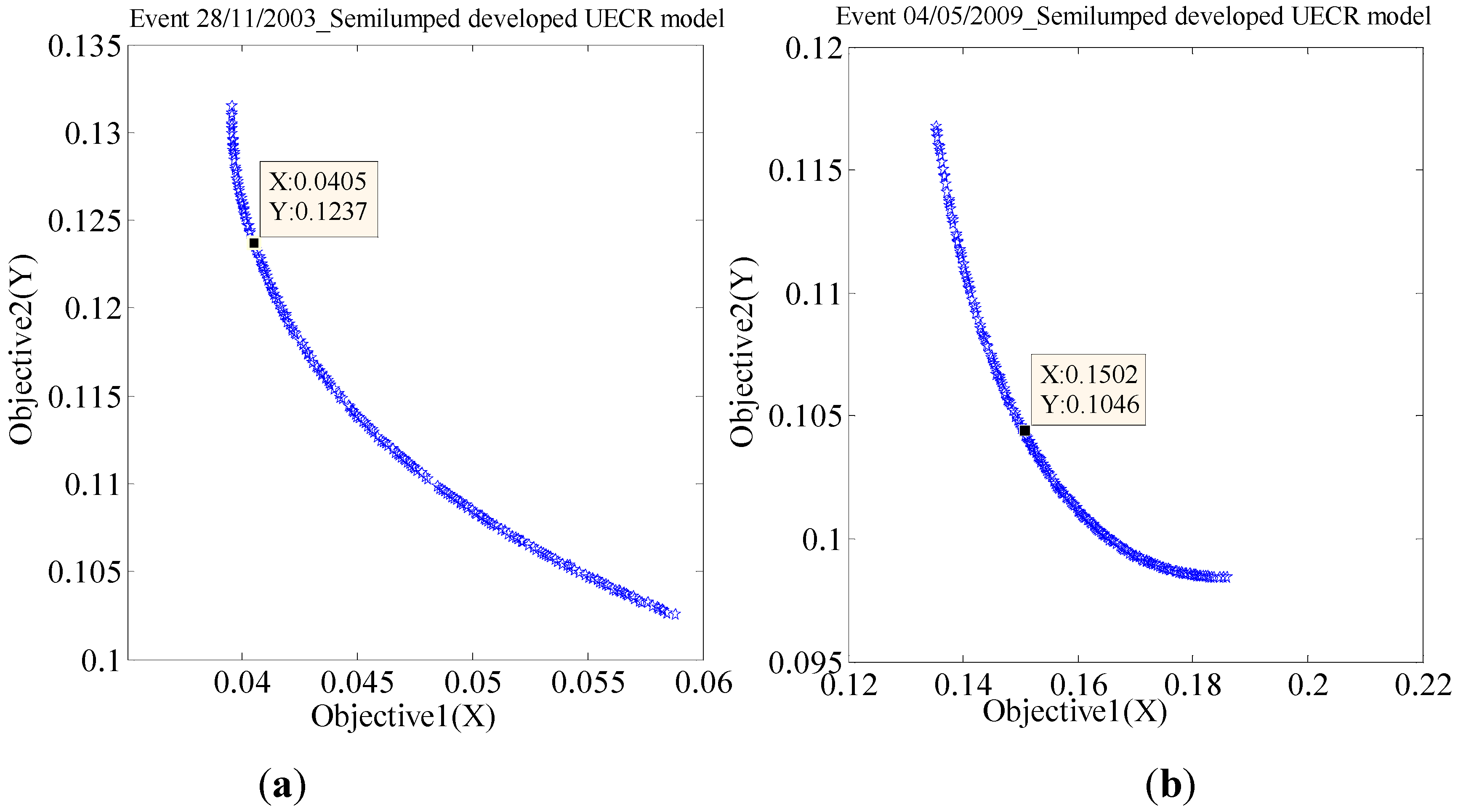
The best compromise solution corresponds to the minimum NRVD and is marked by a point on the Pareto front (Figure 6). In order to find the best compromise value, various computation runs were conducted by changing the population size (150–350), Pareto fraction (0.35–0.9), and distance function to reach a relatively regular and smooth Pareto front. For example, the results of Pareto fronts and related best compromise solutions are shown in Figure 7 for two different events.

Figure 6. Pareto front and best compromise solution. (a) Event 28 November 2003_Semilumped developed UECR model; (b) Event 04 May 2009_seemilumped developed UECR model.

Figure 6. Pareto front and best compromise solution. (a) Event 28 November 2003_Semilumped developed UECR model; (b) Event 04 May 2009_seemilumped developed UECR model.

In Figure 6, X and Y denote the coordinates of the obtained best compromise solutions on the Pareto front in the related Objective 1 (i.e., 1-E₁) vs. Objective 2 (i.e., 1-E₂) space.

Since in addition to excess rainfall being imposed onto the downstream basin as input, the outflow from the upstream basin is also imposed onto the downstream basin as inflow, two-station modeling by considering simultaneous optimization in the upstream and downstream stations could lead to the propagation of the effect of the upstream sub-basin’s parameters and conditions into the downstream sub-basin in which the appropriate estimation of these parameters along with the runoff values in both stations can increase the physical interpretation of the model’s parameters and also reduce the modeling uncertainty. Although the implication of two-objective optimization (multi-site optimization) may lead to a subtle reduction of the modeling performance in the outlet in comparison to the single site optimization (this is the cost of imposing more constraint onto the optimization to obtain parameters with high physical meaning instead of full conceptual parameters due to using more observation data and physical information from inside the watershed), it is logically expected that the implication of the observed data of two or more sites in the multi-site optimization framework could lead to obtaining better a performance in the interior parts of the watershed, especially via a semi-distributed model such as the developed UECR model. This semi-distributed model is able to compute discharge values into the inside points of the watershed (in the outlet of each sub-basin via Equation (11)).

In the following sub-sections the obtained results are discussed and compared based on three aspects of the modeling of the research questions. In this regard the detailed multi-site optimization results are shown diagrammatically in Figure 7, Figure 8, Figure 9 and Figure 10 for simplicity of visual inspection.

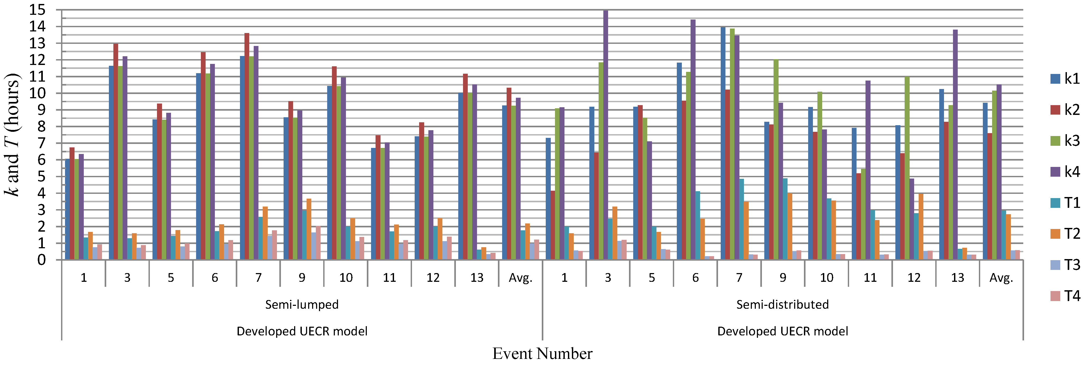
Figure 7. Values of k and T parameters in the UECR model.

Figure 7. Values of k and T parameters in the UECR model.

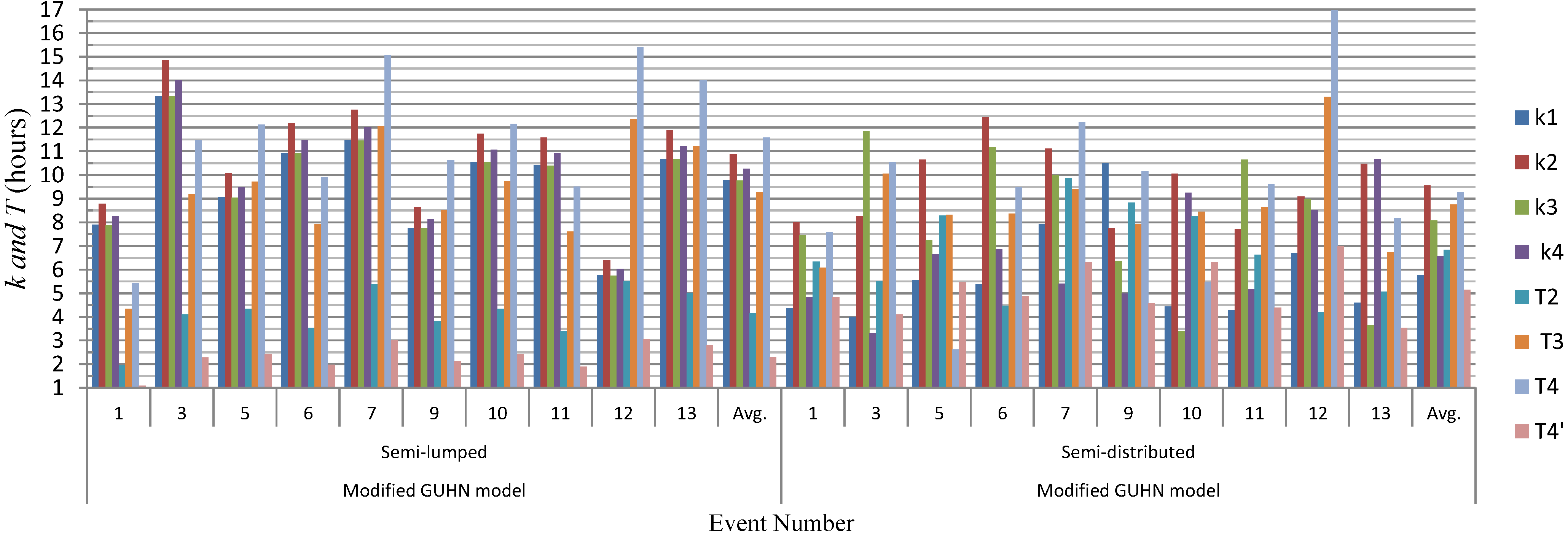
Figure 8. Values of k and T parameters in the modified GUHN model.

Figure 8. Values of k and T parameters in the modified GUHN model.

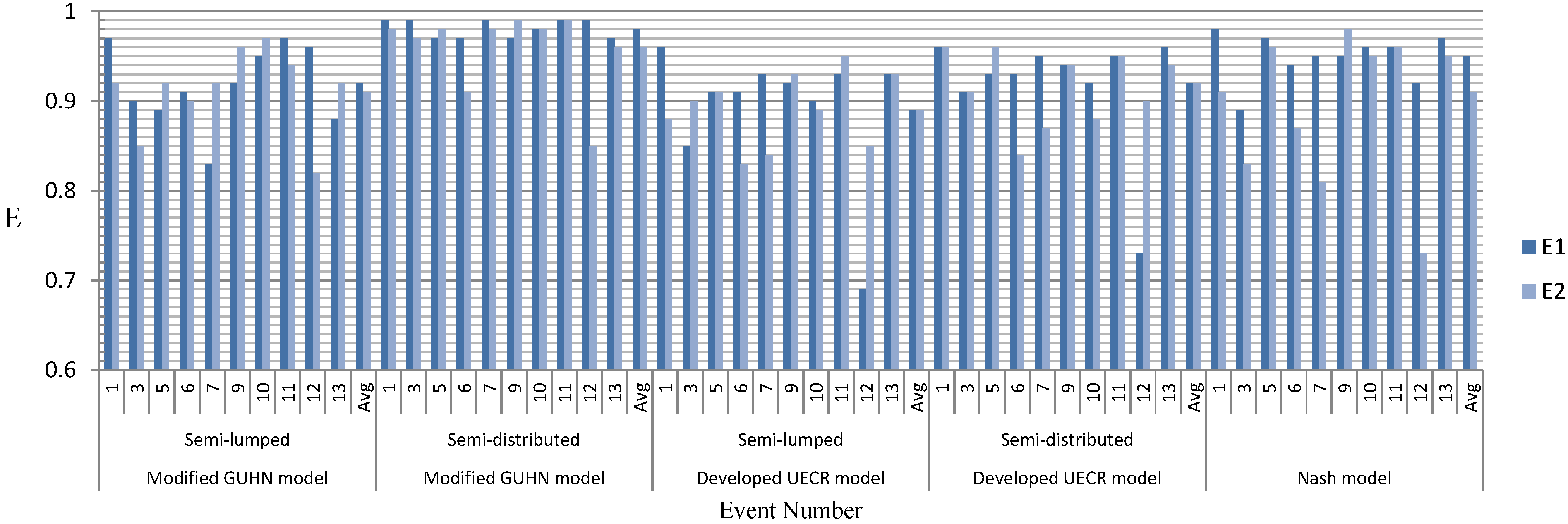
Figure 9. Calibration results.

Figure 9. Calibration results.

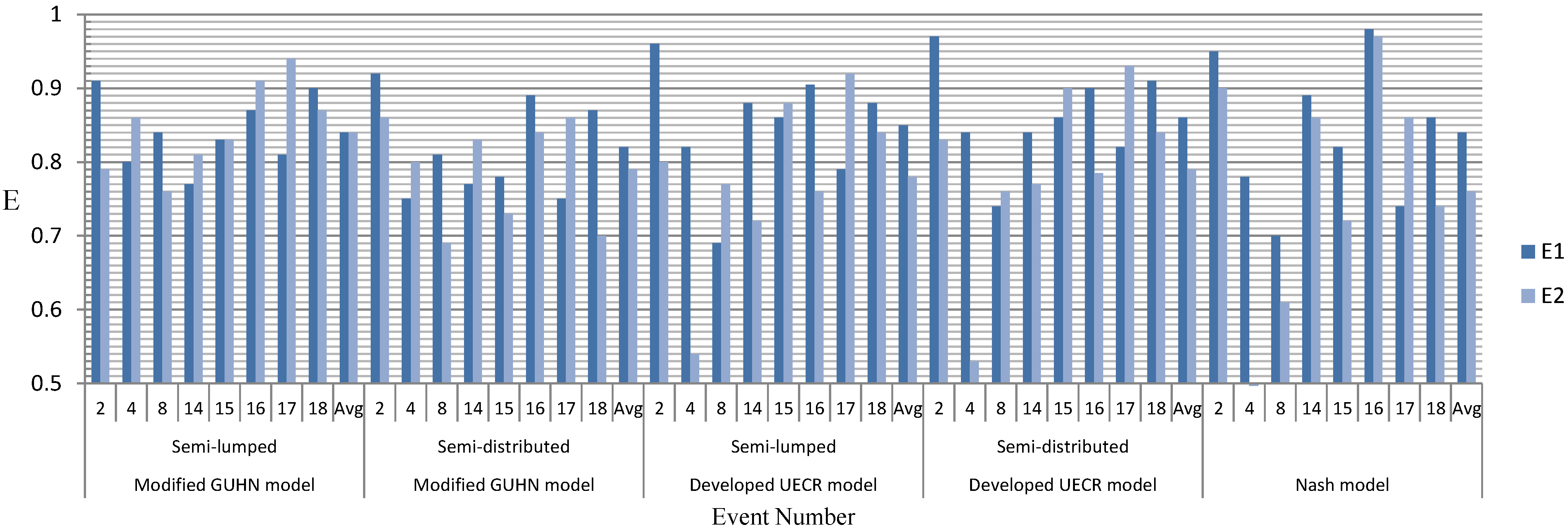
Figure 10. Verification results.

Figure 10. Verification results.

4.1. Comparison of Results between Different Models

The overall results of the two proposed models (the modified GUHN model and the developed UECR model) and the Nash’s traditional model were compared. The optimization results for three parameters (n, k, c,in the semi-lumped strategy) and twelve parameters (k₁, k₂, k₃, k₄, n₁, n₂, n₃, n₄, T₂, T₃, T₄, T₄',in the semi-distributed strategy) of the modified GUHN model, two parameters (a, b ,in the semi-lumped strategy) and eight parameters (k₁, k₂, k₃, k₄, T₁, T₂, T₃, T₄) in the semi-distributed strategy) of the developed UECR model and four parameters of Nash’s model (n₁, n₂, k₁, k₂), presented in Figure 7, Figure 8, Figure 9 and Figure 10 indicate reasonable performance values in the calibration process with slightly better results for large number parameter models, because more degrees of freedom may give better fit of model to the observed data. This way, the results show that calibration via the semi-distributed scenario for the modified GUHN model could lead to a slightly better performance in both stations during the calibration step. However, probable errors existing in the determined parameters may lead to a decrease of the accuracy of the model in the verification process. This issue may be the reason for the slight decrease of the efficiency criterion in all the models during the verification phase, as shown in Table 6 or Figure 10.

4.2. Comparison of Results between Downstream (Station 1) and Upstream (Station 2) Stations

Simultaneous optimization of the models using the observed data of two stations resulted in reasonable efficiency values in both calibration and verification steps along with slightly poor outcomes obtained for the upstream station due to the presence of more uncertainty (Figure 9 and Figure 10).

During the verification step, both calibration strategies of the developed UECR model gave slightly better performances for Station 1, but for Station 2, the modified GUHN model in the semi-lumped strategy slightly outperformed the other models.

The slightly poor results of the Nash’s model in the upstream station in comparison to the other models may be due to the lack of the T parameter in the modeling of an elongated watershed such as the South Fork Eel River (according to Table 5 and Table 6 and Figure 1).

4.3. Comparison of Results between Two Calibration Strategies

The semi-lumped calibration results imply that the hydrological response of the sub-basins varies depending on the seasons when the storms happen. In this regard, as seen in Figure 7 and Figure 8, in the two periods of autumn-winter and spring, the lag times of the events in spring (Events 3, 6 and 7) were obviously longer than others, due to the land cover condition. This indicates that the proposed semi-lumped models, which include geomorphological characteristics, were able to detect seasonal changes of lag times for sub-basins. Also, the results demonstrate that the Nash model was unable to identify such changes properly due to its inherent lumped nature.

Based on the geomorphologic relations (Equations (6) and (12)), it is logically expected that the lag time parameter (k_i) of the large sub-basins are longer than those of the small area sub-basins. As in the relations, the effect of area (A_i) with the exponent equaling 0.3 is larger than the effect of flow length path (L_i) with an exponent equaling −0.1. Therefore, for example k₂ > k₁ and k₄ > k₃ in the modified GUHN and develop UECR models, are to be expected. Besides, in Equations (7) and (13) it is logically expected that the linear channel lag time parameter (T_i) of the large sub-basins with long flow paths are longer than those of the small sub-basins with short flow paths due to the fact that in the related equations, the effect of flow length (L_i) with the exponent equaling one is larger than the effect of the stream slope (S_ti) with the exponent equaling −0.5. Hence, for example T₂ > T₁ in the developed UECR model and T₄ > T₃ > T₂ in the modified GUHN (Figure 7 and Figure 8) are expected. These issues can clarify the difference between performances of two calibration strategies, as will be described in the following.

In the semi-lumped strategy, few parameters (here, two in the develop UECR and three in the modified GUHN) were calibrated for the whole basin that were applicable to other delineated sub-basins if the watershed was divided into more sub-basins. In the semi-distributed strategy, a number of parameters was calibrated that could present the spatial variability of model parameters over the sub-basins, however, due to the lack of the geomorphology relations in the model and the usage of conceptual parameters, there are no physical constraints in these parameters' computation; therefore, this might lead to illogical parameter values in some events (e.g. k₁ > k₂ in both models; T₃ > T₄ in modified GUHN model; T₁ > T₂ in the developed UECR model), as discussed above (see Figure 7 and Figure 8). In this regard, despite good performances, the semi-distributed calibration strategy in some events and for both models was unable to either detect seasonal impacts on the parameters or to properly identify the differences between the parameter values of sub-basins due to sub-basin size and flow path length. The reason for this is related to the direct calibration of pure conceptual parameters of the models instead of using geomorphological relations (or physical parameters) in the models. It is clear from Figure 9 and Figure 10 or Table 6 that the difference between calibration and verification results in the semi-lumped strategy is smaller than the same type difference in the semi-distributed strategy, which indicates a proper and stable structure of the semi-lumped strategy.

On the whole, the overall results showed that the semi-lumped calibration strategy outperformed the semi-distributed calibration strategy in the modeling. It is important to mention that the South Fork Eel River watershed is a nearly homogenous basin with respect to physical characteristics, which means that assuming uniform parameter sets for different sub-basins (i.e., semi-lumped calibration strategy) is not a bad assumption. This is in agreement with results reported by Ajami et al. [53] in a continuous-based semi-distributed modeling.

Applying the proposed models to a more heterogeneous basin along with using proper geomorphological relations in each sub-basin may generate different results when the calibration strategy is semi-distributed.

5. Conclusions

Multi-site calibration was carried out to catch more physically-based parameters of proposed modified GUHN and developed UECR models to improve the routing capability of models in the interior parts (outlets of sub-basins) of the South Fork Eel River watershed, located in northwestern California. Application of more observed data and physical information from inside of basin via multi-site optimization can lead to obtaining reliable parameters with important physical meaning. Contrary to a multi-site model, single-site models cannot properly connect the model parameters to the physical characteristics and will not, consequently, have a clear physical meaning. In order to numerically show the superiority of a multi-site modeling in comparison with single-site modeling for interior parts of basins, it is suggested to perform a cross-validation analysis for a watershed with at least three stations (two for multi-site optimization and one for cross-validation purposes).

In this application, two calibration strategies as semi-lumped and semi-distributed, introduced herein with and without employing the geomorphological relations, were taken into consideration. The calibration results indicated that the semi-distributed calibration strategy for the modified GUHN model slightly outperformed the other models due to the considerable number of parameters involved in the model and more degrees of freedom. The verification results showed that both calibration strategies of the developed UECR model gave slightly better performances for the downstream station, but for the upstream station, the modified GUHN model in the semi-lumped strategy slightly outperformed the other models. In most cases, the obtained performance values for the upstream station were lower than those for the downstream station during verification, which may be due to the presence of more uncertainty. The calibration results also showed that the semi-lumped calibration strategy is capable of identifying seasonal variability of reservoir lag times and also of detecting the impacts of sub-basin size and related flow length path on the parameter values and their discrepancies due to applied geomorphological relations in the modeling framework. On the other hand, semi-distributed calibration of all models was unable to appropriately detect such a variability.

In this study, the averages of the model parameters obtained in the calibration step were used for the evaluation in the verification phase. It is suggested to find just one parameter set valid for all calibration events, considering an aggregated objective function and then using this set for verification.

Simplified models, like the models presented in this study, are the main core of most of the advanced and complex hydrological models. Such new simplified models with reasonable calibration and verification performances can be employed by hydrologists to improve the performance of the available models or to develop other advanced models.

The IUH-based modeling of rainfall-runoff focused on in the present study was performed over short-term storm events. However, the examination of both calibration strategies in the continuous-based runoff simulation using appropriate data (e.g. evapotranspiration, infiltration, subsurface flow, etc.) can be considered as a research basis for future studies.