Assessing Climate Change Impacts on Water Resources and Colorado Agriculture Using an Equilibrium Displacement Mathematical Programming Model

Abstract

This research models selected impacts of climate change on Colorado agriculture several decades in the future, using an Economic Displacement Mathematical Programming model. The agricultural economy in Colorado is dominated by livestock, which accounts for 67% of total receipts. Crops, including feed grains and forages, account for the remainder. Most agriculture is based on irrigated production, which depends on both groundwater, especially from the Ogallala aquifer, and surface water that comes from runoff derived from snowpack in the Rocky Mountains. The analysis is composed of a Base simulation, designed to represent selected features of the agricultural economy several decades in the future, and then three alternative climatic scenarios are run. The Base starts with a reduction in agricultural water by 10.3% from increased municipal and industrial water demand, and assumes a 75% increase in corn extracted-ethanol production. From this, the first simulation (S1) reduces agricultural water availability by a further 14.0%, for a combined decrease of 24.3%, due to climatic factors and related groundwater depletion. The second simulation (S2-WET) describes wet year conditions, which negatively affect yields of irrigated corn and milking cows, but improves yields for important crops such as non-irrigated wheat and forages. In contrast, the third simulation (S3-DRY) describes a drought year, which leads to reduced dairy output and reduced corn and wheat. Consumer and producer surplus losses are approximately $10 million in this simulation. The simulation results also demonstrate the importance of the modeling trade when studying climate change in a small open economy, and of linking crop and livestock activities to quantify overall sector effects. This model has not taken into account farmers’ adaptation strategies, which would reduce the climate impact on yields, nor has it reflected climate-induced shifts in planting decisions and production practices that have environmental impacts or higher costs. It also focuses on a comparative statics approach to the analysis in order to identify several key effects of changes in water availability and yields, without having a large number of perhaps confounding assumptions.

1. Introduction

The agricultural economy in Colorado is dominated by livestock production and sales, which account for 67% of total receipts. Crops, including feed grains and forages, account for the remainder. Most cropping receipts are based on irrigated production, which is sourced from groundwater, especially from the Ogallala aquifer, and surface water, which comes from runoff of snowpack in the Rocky Mountains. Currently, about 86% of water resources are in agriculture, but this is projected to decline due to demographic factors that lead to increased Municipal and Industrial (M&I) water demand, economic factors related to higher costs of irrigation, increased water demand for oil shale mining, and geographic factors such as climatic changes and groundwater depletion. Moreover, hydrologic studies point to an expected decline in runoff from 6% to 20% by 2050, and also a shift in the timing of that runoff to earlier in the spring. These studies also showed that late-summer flows may be reduced [1,2,3,4].

Colorado agriculture has blossomed with the development of water resources used for growing crops, which, in turn, spurs value-added production in the meat and dairy subsectors. Yet, increasing urban development is expected to create a reallocation of 740 million m³ (hereafter million = M) of agricultural water to new municipal and industrial demands by 2030 [5]. Another challenge to the agricultural sector is a possible expansion of ethanol production in Colorado. Shifting corn to ethanol use rather than animal feed could place livestock production, Colorado’s dominant agriculture industry, at a disadvantage as the key input becomes more expensive, even though dry distillers’ grains mitigate some of the constraint. These pressures on agriculture may be exacerbated by the presence of climate change, particularly its effect on water availability and yields. Stakeholders thus seek ways to better understand the implications of climate change on statewide water availability and requirements for crops and livestock, in the presence of a larger population and other new demands such as ethanol production. This research evaluates these issues with illustrations on how resources might be reallocated and how prices respond in the future.

The research uses a positive mathematical programming model specified to represent the Colorado agricultural sector, which is simulated to examine impacts of selected future constraints on water and yields resulting from climate change. First, this model was calibrated to 2007 quantities and prices. Then, a “Base” scenario was constructed, which reflects several future drivers of change affecting the state’s agriculture: (1) increasing competition for water due to population growth, especially shifts in the resource from agricultural to municipal uses in the South Platte and Arkansas River basins; and (2) we also add two ethanol plants into the South Platte River Basin, which leads to a 75% increase in corn extracted-ethanol production there, and provides competition to the cattle feeding industry’s use of a key input, corn for grain.

The changes incorporated into the Base scenario are related to the anticipated growth in the local economy, but to do not include effects of climate change. With this Base established, we run three simulations to explore the implications of climate change. The first one further reduces water availability based on forecasts of reduced runoff, while the second and third simulations introduce yield changes that might arise due to higher temperatures and increased variability of rainfall. Results for these scenarios are reported in terms of acreage changes, total value of production, exports and imports from the state, and prices. The overall changes in consumer and producer surpluses across the simulations are also reported. This modeling effort does not attempt to capture the full set of dynamic effects that will in fact occur, because for a small region, the range of possible outcomes over the next several decades is high, and is dependent on an equally extensive set of possibilities. Our approach is thus to focus on important outcomes with regard to climate change using a comparative statics method.

The document is organized into a series of sections. The current status of Colorado agriculture and its dependence on irrigation water supplies is reviewed in Section 2. This section also includes a review of expected climate change impacts on the availability of water and effects on commodities. Section 3 provides a literature review with regard mathematical programming methodology, while Section 4 lays out our particular model. Section 5 provides a discussion of the simulations and results, and Section 6 gives conclusions and thoughts for further research.

2. Colorado Agriculture and Water Use: Current and Projected Changes

This section contains two parts: the first covers the current size and structure of Colorado agriculture and describes key changes that might occur over the next decades; the second looks at the current pattern of water use and reviews forecasts of water reallocation.

2.1. Agriculture in Colorado

The agricultural economy in Colorado is dominated by livestock (almost $5.8 billion in sales during 2007, the year used to calibrate our model), which accounts for 67% of total receipts from the sector. The 2007 commodity balances are contained in Table 1. Colorado agriculture is heavily traded outside the state and abroad, as we learned when building commodity balance sheets used in the model. Fed beef, the largest economic sector, produced $3.4 billion in 2007 and traded 82% of its production out of state. The cattle feeding industry creates a substantial derived demand for corn production ($463 Million hereafter M) and corn imports, which reached $703 M in the same year. In 2007, 75% of the total value of Colorado’s crops came from irrigated acreage, as most of hay, corn, and pasture for livestock were produced on irrigated land [6].

Table 1. Production, in-state sales, exports, and imports of key Colorado agricultural commodities.

Crop or Commodity	Production (M $)—Co1umn 1	In State Sales (M $)—Co1umn 2	Exports (M $)—Co1umn 3	Imports (M $)—Co1umn 4	% Exports/production % of column 3/column 1	% Imports/production % of column 4/column 1
Corn*	462.8	1051.7	113.7	702.6	24.6	151.8
Wheat	483.5	61.0	474.8	52.3	98.2	10.8
Barley	185.3	67.2	163.9	45.9	88.5	24.7
Sorghum	383.7	400.3	0.0	16.6	0.0	4.3
Dry beans	24.7	7.2	17.6	0.0	71.0	0.0
Beef	3382.5	905.6	2748.4	0.0	81.3	0.0
Cow calf	135.8	278.2	0.0	142.4	0.0	1.0
Hogs	170.9	204.0	0.0	33.1	0.0	19.3
Dairy	522.3	566.4	0.0	44.1	0.0	8.5
Sheep	488.5	27.1	461.4	0.0	94.5	0.0
Broilers	145.7	205.4	0.0	59.6	0.0	40.9
Eggs	74.1	85.6	0.0	11.5	0.0	15.5

Note: * Corn sales includes ethanol production.

Table 1. Production, in-state sales, exports, and imports of key Colorado agricultural commodities.

Crop or Commodity	Production (M $)—Co1umn 1	In State Sales (M $)—Co1umn 2	Exports (M $)—Co1umn 3	Imports (M $)—Co1umn 4	% Exports/production % of column 3/column 1	% Imports/production % of column 4/column 1
Corn*	462.8	1051.7	113.7	702.6	24.6	151.8
Wheat	483.5	61.0	474.8	52.3	98.2	10.8
Barley	185.3	67.2	163.9	45.9	88.5	24.7
Sorghum	383.7	400.3	0.0	16.6	0.0	4.3
Dry beans	24.7	7.2	17.6	0.0	71.0	0.0
Beef	3382.5	905.6	2748.4	0.0	81.3	0.0
Cow calf	135.8	278.2	0.0	142.4	0.0	1.0
Hogs	170.9	204.0	0.0	33.1	0.0	19.3
Dairy	522.3	566.4	0.0	44.1	0.0	8.5
Sheep	488.5	27.1	461.4	0.0	94.5	0.0
Broilers	145.7	205.4	0.0	59.6	0.0	40.9
Eggs	74.1	85.6	0.0	11.5	0.0	15.5

Note: * Corn sales includes ethanol production.

It is not possible to say how much imported corn went into ethanol production, but ethanol used the equivalent of 23% of the state’s production, while 67% of corn was imported. The value of wheat production equaled that of corn output, but 98% was exported across state boundaries. The sheep and lamb industry is also heavily export-oriented, with slightly less than $500 M in revenues during 2007, and 94% exported. Sorghum was the largest feed grain produced after corn, with revenues in excess of $380 M and imports totaling about $17 M. Instate sales of corn, excluding the ethanol industry, exceeded $800 M, while sorghum was $400 M. Colorado’s dairy and hog sectors sold output within the state and required imports to meet demand, totaling 8.4% and 19% of production respectively. Imports of cows and calves were 50% of instate calf sales ($278 M) with buyers almost exclusively being feedlots. Barley and dry beans were relatively small agricultural subsectors and produced mostly for exports (88% and 71% of their production respectively). At the other end, 30% of broilers’ sales in Colorado (about $60 M) and 13% of egg sales were imports.

Ethanol production may play a key role in Colorado’s energy future and plans therefore exist to expand production capacity. Yet, Colorado is a small producer of ethanol, with just three plants located in the South Platte River Basin. The average plant capacity in Colorado is 215 M liters per year, or about 1.3% of the nation’s ethanol capacity. The “corn footprint,” or demand by these plants, is approximately 1.6 M tons each year, which requires about 130,000 hectares of irrigated corn production.

Expected Climate Change Effects on Colorado Agriculture. A consensus of climate change models suggest temperature in Colorado is expected to increase by up to 9–11 degrees Fahrenheit in the worst case scenario. The timing of seasons is likely to shift as well, with an earlier spring and longer fall. Midwinter precipitation should occur later in the calendar year, while less rain is expected to fall in late-spring and summer. As temperatures rise, runoff will peak earlier in the spring and be reduced significantly in late summer. Earlier run off could result in an 8.5% reduction of in-stream flows by midcentury in the Colorado River basin and a 5%–10% possible reduction in the Arkansas and Rio Grande basins. Little work has been done for the South Platte in terms of the impact of climate change on winter snow runoff [7]. The variability year to year is also likely to grow.

Climate change will have effects on crop yield and water requirements. The main climate factors affecting agriculture are temperature, availability of water, and the concentration of atmospheric CO₂. Soil water availability depends on the above three factors as they interact with soil properties, while field humidity, clouds and solar radiation also influence plant water requirements. The major commodities in Colorado agriculture are affected variously by these climate factors. For corn, the yield loss associated with increased temperature exceeds the positive effects of increasing carbon dioxide levels, so yields are expected to decline [8]. Also, high temperatures earlier in the season lead to less pollen germination and lower yields [9]. The changing precipitation patterns suggest increased yields for non-irrigated wheat in Colorado given the increase rainfall in winter and early spring.

High temperatures also extend the number of growing degree days in the crop season, which has a positive effect on yields and overall production for hay. However, few studies exist on the effects of climate change for this crop. In a review of three studies, depending on the assumed increase of CO₂ concentration, alfalfa yields were estimated to change from a 16.7% increase to a decrease of 19.4%. However, this added growth and length of season may lead to lower nutritional content, depending on soil quality constraints [10,11]. On the other hand, productivity may be higher than previously expected in semi-arid grasslands, and thus additional forage may become available [12].

Warmer temperatures increase plant evapotranspiration, while CO₂ concentration partially offsets this process by increasing plant water-use efficiency. Wheat and hay are more sensitive to CO₂ than corn [8,13]). Although there is great uncertainty about the future CO₂ concentration, it is unlikely to neutralize the effect of anticipated, protracted droughts on crop production.

Increasing heat also affects livestock growth and performance. Higher temperatures reduce livestock production in the summer but increase it in winter. Under heat stress, animals reduce grazing to stay in the shade, thus reducing their feed intake and suffering from weight loss. Reduced quality of forage and digestibility leads to reduced dairy productivity. The greater the stress, the easier is the spread of parasites and disease pathogens. For dairy cows, heat stress reduces the milk fat and protein content in milk, and the quantity of milk produced is reduced up to 10%; moreover, other factors may also lead to lower yields as high-producing dairy cows are the most susceptible to heat stress due to breeding selection for high productivity, and reproduction rates are also adversely impacted [3,14,15,16].

2.2. Colorado’s Outlook for Water Resources

Competition for water is increasing in the West. Colorado is a headwater state, supplying water through river systems to eighteen downstream states. Interstate compacts mean that Colorado is not entitled to all surface water flows, and may only retain six billion m³ in an average year. This water is allocated among users according to the Prior Appropriation Doctrine, and, as nearly all of Colorado’s rights have been appropriated, new users must obtain rights from others through voluntary transactions. Agriculture is the largest diverter and consumptive user of these surface flows. Agriculture also makes use of groundwater resources so that, on average, 1.0 M hectares of cropland are irrigated via groundwater or surface water. As noted earlier, irrigated crops comprise three-quarters of cropping receipts in Colorado, with two-thirds of these receipts bound for Colorado’s livestock feeding industry [17].

Irrigation water depends on both groundwater, especially from the Ogallala aquifer, and surface water, which comes from runoff due to snowpack in the Rocky Mountains. Currently, about 86% of the state’s water resource is used in agriculture, but this amount is projected to decrease. Causes for decline include demographic factors, such as increased Municipal and Industrial (M&I) water demand, economic factors related to higher costs of irrigation, increased water demand for oil shale mining, and geographic factors such as climatic changes and groundwater depletion.

While agriculture holds the majority of water rights, new demands for water resources come from a growing population and environmental uses. Population forecasts are for an increase of more than 50% in the next twenty years, so a gap between existing municipal water supplies and demand from the larger population is anticipated. The Colorado Water Conservation Board’s Statewide Water Supply Initiative (SWSI) predicts that Colorado’s South Platte Basin will experience a 61.9% increase in water demand, or about 505 M m³, by 2030, which will continue to rise thereafter. With water already appropriated in the South Platte, an estimated 73,000 irrigated hectares will need to be permanently fallowed to supply these increasing demands. The plans for nearly all South Platte water providers include significant water rights transfers [1,18].

Great variation exists among findings of hydrologic studies regarding expected decline in runoff, from 6% to 20% by 2050, although there is consensus on the persistence of the shift of runoff to earlier in the spring, and a change in precipitation to a greater intensity during winter and lesser in spring and summer [1,2,3]. The topography of the state and other factors make projections particularly complex [19].

3. Literature Review

The model used in this research is an optimization model using mathematical programming in a manner that has a long history in economics and engineering. The approach chooses activity levels that maximize an objective function in the face of physical constraints on resources. Positive Mathematical Programming (PMP) improves on earlier techniques by allowing perfect calibration to a base and additions of more realistic behavior into such models [20,21]. As an activity based approach, PMP simplifies communication across disciplines and is particularly suited to study bio-physical and environmental features of agricultural systems.

Over the last 10 years, the PMP approach has been object of extensive review, critique and extensions [22,23,24,25], as policy makers increased their reliance on quantitative economic models to understand effects of agricultural policies. As such, the method has been widely used in sectoral and regional analysis. In the European Union (EU), several models analyzed policy instruments within the EU’s Common Agricultural Policy (CAP), especially the effects of the CAP reform starting in 2003–2004, where a switch to decoupled payments to farmers was made. Some examples of these models include the FAL, Parma and Madrid models, which use PMP to calibrate to observed values, and also apply the maximum entropy approach to estimate total variable costs [26,27,28,29,30,31,32,33,34,35,36].

The PMP method is thus versatile enough to model policy scenarios in a straightforward fashion, and has been adopted as especially well-suited to examine animal feed requirements and land constraints [25], and to study jointly agricultural outputs and environmental externalities [31]. Howitt et al. [32] applied the methodology to estimate effects of climate change on irrigated agriculture in California using the State Water and Agricultural Production model (SWAP). SWAP improves on traditional PMP models by allowing for large policy shocks and enhanced flexibility in handling input substitutions. These models are often linked to hydrological network models and other biophysical system models.

The equilibrium displacement modeling approach [33,34] represents an economic system of demand and supply relationships, and can show the effects of exogenously determined shifts of supply and demand from an initial equilibrium (a displacement). Changes in market prices and quantities resulting from the displacement determine changes in consumer and producer surpluses. This follows originally from Samuelson [35], who shows that maximizing profits is equivalent to maximizing the total surplus when markets are competitive.

The Equilibrium Displacement Mathematical Programming (EDMP) model originally developed by the USDA Economic Research Service Harrington and Dubman [36] is a sector-wide, comparative statics model of the U.S. agricultural sector, applying a mathematical programming approach to the equilibrium displacement methodology, with specific farm sector relationships and policies reflected. They used values estimated by econometric studies and applied the asset-fixity theory of Johnson and Quance [37] to estimate slopes of supply functions. The Harrington and Dubman model is similar to the general PMP approach, but the supply and demand curves are explicit, and the base calibration is achieved by shifting intercepts until they match initial values with as much precision as is needed. Thus this approach is termed an “equilibrium displacement mathematical programming” model.

Regional and Climate Change Studies. Connor et al. [38] noted that an increasing number of analyses assess the impacts of climate change on irrigated agriculture in arid and semi-arid regions of the world, especially those that face a projection of drier weather. The objective function of their irrigation sector model maximizes profits across three sub-regions in the Murray-Darling River basin, Australia, subject to land and water constraints. The scenarios included a base case, a water scarcity model, a water variability model, and full effects model. The latter model includes both water variability and implications for changes in salinity. They concluded that ignoring the combined water-climate effects, along with salinity, leads to results that understate costs and impacts on output. Moreover, using the analysis of salinity, they identify various thresholds of climate change that create structural change in productivity and costs related to levels of salinity.

Henseler et al. [39] studied global change in the Upper Danube basin using an agro-economic production model, with two climate change scenarios. The first scenario assumed a significant increase in temperature, while the second one showed effects of a moderate increase. This study’s results showed large differences in agricultural income and land use between the two scenarios and shifts that lead to increases in cereal production and extensive grassland farming due to the increased temperature in the first scenario. Qureshi et al. [40], Whitney and van Kooten [41], and Wolfram et al. [42], studied climate change impacts on agriculture at the regional levels in Canberra Australia, Western Canada, and California respectively. These studies reached conclusions that are similar to the studies discussed above. Whitney and van Kooten [41] expanded the model to include impacts on pasture and wet-land.

Finally, with regard to previous Colorado analyses, Bauman et al. [43] estimated the economic impacts of the drought in 2011 using an Input–Output (I/O) model and a variant of the current Colorado Equilibrium Displacement Model. The authors found that the 2011 Colorado accounted for $83 to $100 M in economic impact, when all economic sectors of the state economy were included. Schaible et al. [44] argued that the gradual warming in the Western United States is expected to shift the precipitation pattern and alter the quantity and timing of associated stream flows. In addition, the effects of climate change will move bio-energy growth to the Ogallala aquifer in the Western States, which demand that careful optimization of water use is needed to choose irrigation technologies. They underline the importance of further research to understand economic implications of climate change at the regional level.

Thus, previous studies agreed that there are likely to be significant shifts in land use and crop mix due to climate changes at the regional level. These studies also agreed on the importance of understanding possible structural changes, and noted that there will be significant income and price effects due to climate change. Furthermore, the above review suggests that a lack of studies investigating the impact of climate change at the regional level exist, in particular those that trace out impacts in a small, open economy via trade with the Rest of the World (ROW) and include livestock and crop interactions. Previous studies also agree that positive mathematical modeling fits the research problem and unveils opportunity to simulate possible production and cost changes due to climate change, which should enable a better understanding of welfare implications at the regional level.

4. Structure of the Colorado Equilibrium Displacement Positive Mathematical Programming (Colorado EDMP) Model

The Colorado Equilibrium Displacement Positive Mathematical Programming model (Colorado EDMP) is a variant of the EDMP model by Harrington and Dubman, which the authors adapted for Colorado’s agricultural sector [45]. This model maximizes the sum of producer and consumer surpluses across most major products in Colorado’s agricultural sector, subject to a number of spatial market and resource constraints. The Colorado EDMP is calibrated to Colorado’s agricultural economy, and adds other natural resource dimensions (i.e., Colorado agricultural sector demand for water). Spatial constraints consist of three regions with separate water availability for irrigation in each basin (South Platte River basin, Arkansas Basin, and other Colorado basins) along with differing crop water requirements in each basin. These requirements were developed using irrigation water requirement (IWR) coefficients per crop per region from the Colorado Decision Support System (CDSS) weather and soil characteristics databases [46]. The optimization model selects food and feed crops, water supplies, and other inputs to maximize the sum of producer and consumer surpluses, subject to constraints on water and land, and subject to economic conditions regarding prices, yields, and variable costs. In the following paragraphs, we describe the Colorado EDMP and its basic dimensions.

The particular function given below is a second order Taylor series expansion as first introduced by Takayama and Judge [47], which permits an approximation of an unknown functional form for the cost function:

Max: Z = F^′x − 1/2 x^′ H x

(1)

with x > 0, where x is a vector of endogenous variables that relate to sector demand and production processes. In the following expanded form of the Equation (1), the vectors x are divided into five groups. In the notation below the vectors of variables are written in lower case, while the vectors of parameters are in upper case, and indices under the summation operators are simplified as:

Z = ∑_j(F^″ − .5Hq_j)q_j − ∑_i∑_b(F^″ + .5Hcl_i)cl_i − ∑_nu + ∑_g(F^″ − .5He_g)e_g − ∑_s(F^″ − .5HM_s)M_s

(2)

where, q_j = domestic sales of j agricultural commodities (in M tons) and livestock products (M head, tons, or dozens of eggs); cl_i = feed and food crop activities i identified by river basin (for selected crop activities, in M hectares) and livestock activities (head counts, live weight, milk tons and dozens); u= dollar value of n inputs (in M dollars); e_g = exports of t agricultural commodities (in M tons) and livestock products (M tons, dozens of eggs); M_s = imports of s agricultural commodities (in M tons) and livestock products (M tons, dozens of eggs); F^″ = a vector of intercepts indexed under each set above, which are determined in the calibration phase; H = the diagonal elements of the Hessian matrix flowing from the First Order Conditions. H is assumed to be negative semi-definite.

In Equation (2), the first term is the function of total revenue, where (F^″ − .5Hq_j) = p is the vector of price dependent domestic demand functions, and p is the vector of output prices. The H_j elements are derived from predetermined elasticities of demand for j commodities and livestock products. The second element is a non-linear total variable cost function, where H_ib are elements of the Hessian of supply functions; they are calculated as the ratios of capital replacement costs over excess capacity for i activities in b river basins. The term (F^″ + .5Hcl_i) = Marginal Cost provides the supply side equivalent to a price dependent demand function in the first term. The third element is the sector’s sum of inputs used in the sector, entered in value terms. The last two elements represent the export and import functions (these include out-of-state trade as well as international trade), which are included in the sector’s the objective function (see also Helming [48]). Ht and Hs are also exogenously calculated. Examples of the constraints included in the mathematical program are presented in Appendix.

The agricultural activities in the model cover 91% of total agricultural production in Colorado, including thirteen crop and nine livestock commodities, which are sold to local consumers or out-of-state exports. Imports for nine products are present and compete with local production. The nine livestock sectors are cow calf, fed beef, hogs, dairy, sheep, broilers and layers, turkeys, and horses. Some of these livestock activities produce multiple products, including meat, milk, and/or eggs. Demand for feed crops and forages are derived from livestock activities through demand for rations. Food crops are wheat, potatoes, sunflower, and dry beans. Calf imports go directly into the cattle feeding industry. The commodities included, their acreage and production values, and a comparison of how our calibrated model compares to historical 2007 values is given in Appendix

Table A1. Area and production of crops and livestock activities, actual, and calibrated values for the Colorado EDMP.

Crop or Commodity	Units	Historical 2007 quantity	Calibrated quantity	Hessian element	Intercept
Ethanol	Million Liters	648.97	660.96	0.00	1.51
South platte dry corn	Million Hectares	0.10	0.11	−76.73	909.07
South platte irrigated corn	Million Hectares	0.21	0.23	−38.93	1173.13
Arkansas dry corn	Million Hectares	0.04	0.13	−81.46	436.30
Total corn	Million Hectares	0.36	0.47
South Platte dry wheat	Million Hectares	0.04	0.00	−183.25	1160.79
South Platte irrigated wheat	Million Hectares	0.55	0.63	−11.25	1549.58
Arkansas dry wheat	Million Hectares	0.33	0.31	−22.30	703.28
Wheat, other a	Million Hectares	0.04	0.00	−157.75	2262.93
Total wheat	Million Hectares	0.87	0.93
Sorghum	Million Hectares	0.07	0.07	−44.27	1683.21
Potatoes	Million Hectares	0.02	0.03	−13871.39	4041.04
South Platte irrigated. hay, all	Million Hectares	0.15	0.12	−10.04	1077.62
Arkansas dry hay, all	Million Hectares	0.09	0.11	−121.73	1082.96
Hay all, other	Million Hectares	0.31	0.34	−9.71	3251.96
Hay all, total	Million Hectares	0.55	0.57
Fed beef	Thousand Ton	1235.6	1241.9	−0.2	182.1
Hogs,	Thousand Ton	161.6	165.7	−57.3	76.4
Dairy	Thousand Ton	1228.3	1236.5	−1.1	42.3
Broiler	Thousand Ton	157.5	173.4	−6.1	92.8
Eggs, independent	Million dozens	8.83	9.72	0	1.9
Eggs, contracted	Million dozens	79.5	87.45	0	2.5
Turkey, independent	Thousand Ton	13.6	16.8	−108.3	108
Turkey, contracted	Thousand Ton	20.9	21.3	−141.3	135.4

Note: ^a Other basins include San Luis Valley and Colorado River basin.

.

The model also includes accounting costs for all activities. Inputs are categorized in the following categories: genetic inputs, such as seed or calves; specialized technology; mineral fertilizers (without manure applications); other chemicals; fuel and lube; electricity; irrigation energy and other irrigation costs; other variable purchased inputs; fixed cash costs; and capital replacement costs. Farm production costs reflect various yields and cost structures in different basins. Irrigated and non-irrigated crop costs are derived from enterprise budgets created by extension professionals in Colorado and the High Plains. Currently, the relationship between inputs and outputs is fixed, with no substitution, so that corn production, for example, has a fixed yield of 8.3 tons per hectare and each hectare uses a certain quantity of fertilizer, other chemicals, and irrigation energy (when irrigated).

Demand elasticities from the literature provide the values for the Hessian’s elements related to demand, which help the model, provide reasonable responses when used in scenario analyses. The F values, or intercept terms, are estimated by repeated adjustments until the prices and quantities are calibrated to a desired level of accuracy.

It is possible, with enough time, to exactly calibrate prices and quantities by shifting demand and supply intercepts. While this can be a tedious process, it provides an examination of the relationships and tendencies in the model, which cannot be achieved as intuitively when using a large set of cross price elasticities that, in any case, cannot be reliably identified for a small region like Colorado. We show the results of our efforts at calibration in Appendix Table A1, where the table shows the calibrated quantities versus actual values for selected products. It also provides estimates of the intercepts and slopes (Hessian elements) of the associated supply curves.

5. Base Scenario and Climate Change Simulations

This research includes three climate change simulations that are compared to the Base simulation, where the “Base” is designed to represent selected features of the sector several decades in the future. The two main features included are reduced water availability in the South Platte and Arkansas River basins, and added demand for ethanol, which represents a competing demand for corn. Three simulations then are created to show incremental effects of climate change on the Base model. The first simulation (hereafter S1) reduces agricultural water availability by a further 14.0% across all basins, for a combined decrease of 24.3%. This reduction comes from climatic factors and related groundwater depletion, as detailed in the Colorado Water Conservation Board’s Statewide Water Supply Initiative study (CWCB) [2]. There are no changes in yields or other factors.

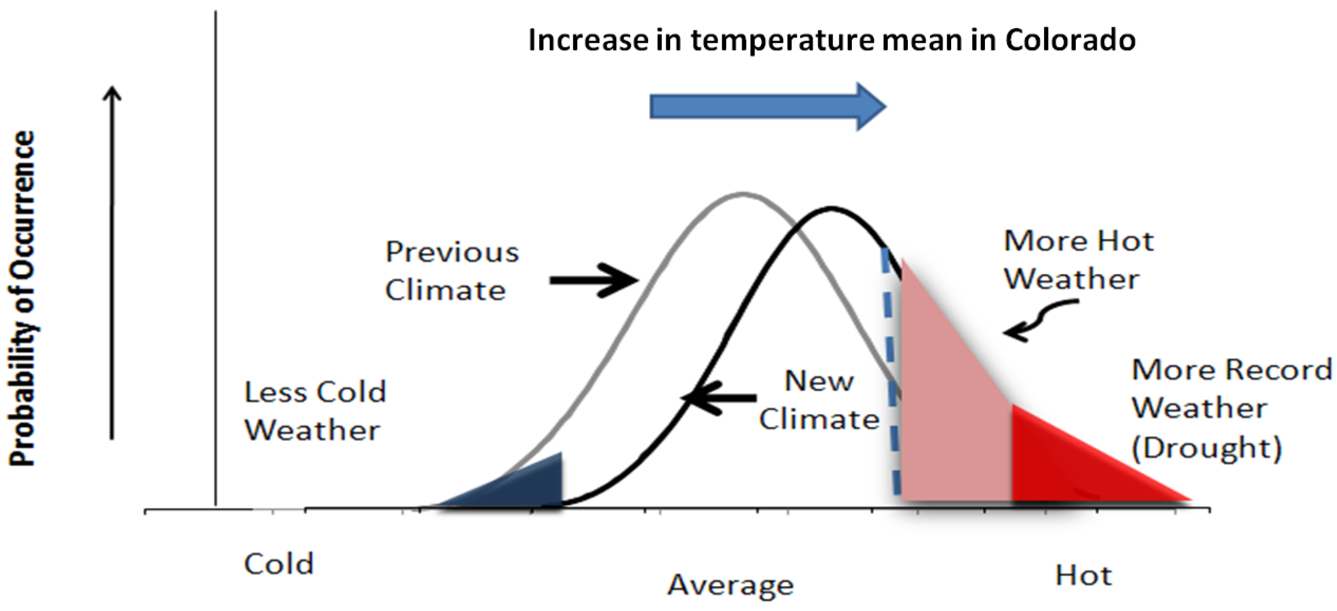
In addition to the direct water reduction, the effects of increased heat and an extreme dry year are reflected in the second and third simulations. First, climate change models suggest up to a 9–11 degree Fahrenheit increase in temperature, as a high end case [23]. The average rise in temperature also affects the variability and likelihood of years with more extreme weather, as illustrated in Figure 1. This figure illustrates how the increase in average temperature leads to a greater likelihood of extreme weather events, such as droughts, but also to years with higher precipitation. Simulation two represents a warm and wet year (hereafter S2-WET), with shifts in the pattern of precipitation, but with an increase in average temperature included as well. The third simulation reflects a drought year (S3-DRY) with dry conditions, in addition to the temperature increase and shifts in precipitation found in S2-WET.

Table 2 summarizes the percentage changes in crop yields and dairy productivity from those used in S1. The irrigated corn yield in S3-DRY decreases due to higher July temperatures, and from lack of rain and cloud cover, which hampers pollination [8]. Yields for non-irrigated wheat increase as sufficient winter rainfall is present s during the critical growing period in S2-WET, and decline by an equal amount in S3-DRY to reflect the effect of less rainfall and higher temperatures [13].

Both irrigated hay and corn silage yields surge with higher temperatures, which result in a longer growing season and more cuttings, in the case of hay, and help biomass growth in silage. Because both are grown on irrigated land, decreased rainfall does not have an effect, and yields are kept high in both scenarios. Yields in rangeland and pasture increase in S2-WET year, as sufficient rainfall supports germination and growth, but like other non-irrigated crops, these sources of feed see reduced yields in S3-DRY. Dairy sector productivity plummets in both the second and third simulations, reflecting animal stress from high temperatures in absence of mitigating strategies. (These impacts of climate change are presented in more detail in Section 2).

Table 2. Percent yield and productivity changes in S2-WET and S3-DRY, relative to S1. Sources: [13] (pp. 34–48, 56–61, 77–82).

Simulation	Irrigated corn	Dryland wheat	Irrigated hay	Silage	Pasture	Rangelands	Dairy
S2-WET	−0%	13%	18%	13%	8%	8%	−18%
S3-DRY	−15%	−13%	18%	13%	−13%	−13%	−18%

Table 2. Percent yield and productivity changes in S2-WET and S3-DRY, relative to S1. Sources: [13] (pp. 34–48, 56–61, 77–82).

Simulation	Irrigated corn	Dryland wheat	Irrigated hay	Silage	Pasture	Rangelands	Dairy
S2-WET	−0%	13%	18%	13%	8%	8%	−18%
S3-DRY	−15%	−13%	18%	13%	−13%	−13%	−18%

In summary, the following conditions are analyzed in the next sections:

Base: This scenario examines the economic impacts of shifting water resources from agricultural to municipal uses in the South Platte and Arkansas River basins by 22% and 18% respectively;

S1: This simulation alters the Base scenario by reducing agricultural water availability by a further 14.0% across all basins for a combined decrease of 24.3% based on expected climate change effects;

S2-WET: This simulation represents a warm and wet year, with shifts in the pattern of precipitation and an increase in average temperature;

S3-DRY: A drought year is simulated in the third example, using dry conditions along with the temperature increase and shifts in precipitation found in S2-WET.

Figure 1. Climate change scenarios in Colorado Economic Displacement Mathematical Programming (EDMP).

Figure 1. Climate change scenarios in Colorado Economic Displacement Mathematical Programming (EDMP).

Note: Relatively small shift in the average climate can substantially increase risk of extreme events such as drought [4].

Base Scenario. The Base scenario reflects selected supply and demand factors for agricultural inputs and outputs in the future. First, it includes expected implications of competition between the agricultural sector and other sectors (e.g., M&I) for water at the basin level. In particular, this scenario shifts water resources from agricultural to municipal uses in the South Platte and Arkansas River basins by reducing water availability to agriculture by 22% and 18% respectively, with respect to calibrated values for 2007. This reduction follows estimates by the Colorado River Water Availability Study—CRWAS-report [49], and results in the fallowing of a proportional amount of irrigated land in each basin, although individual crops can vary without constraint aside from the overall reduction in irrigated acreage. Overall a net decrease of 10.3% in total water availability occurs because nearly 50% of annual volume is in river systems outside of these two basins.

Additionally, this simulation adds two ethanol plants in the South Platte River Basin, thereby increasing Colorado ethanol production from 175 M gallons annually to 308 M gallons. The Base scenario values are found in Table 3 and Table 4.

Base Scenario Results. Due to an anticipated reallocation of water from agriculture to municipal uses in the South Platte and Arkansas basins in the Base scenario, crop acreage shifts relative to the calibrated values of 2007, particularly for those commodities that are produced on irrigated land. Also, adding two ethanol plants raises annual production from 662 M liters annually to 1165 M liters. This increase raises demand for corn by about 1168 k tons (hereafter thousand = k), which must be supplied from various sources. On the one hand, other uses of corn can decrease, which in this model are feed, final consumption and exports. Also, supplies can come from added production or greater imports.

Table 3. Area harvested in Base scenario and Climate Change Simulations.

Crop/Livestock product	Base	Simulation			Percentage change from Base
		S1	S2-WET	S3-DRY	S1	S2-WET	S3-DRY
South platte dry corn	0.07	0.07	0.06	0.1	0.0%	−14.3%	42.9%
South platte irrigated corn	0.27	0.26	0.25	0.17	−3.7%	−7.4%	−37.0%
Arkansas irrigated corn	0.07	0.07	0.07	0.04	0.0%	0.0%	−42.9%
Arkansas dry corn	0.16	0.17	0.15	0.04	6.3%	−6.3%	−75.0%
All corn	0.58	0.57	0.53	0.36	−1.7%	−8.6%	−37.9%
South platte dry wheat	0.62	0.65	0.65	0.33	4.8%	4.8%	−46.8%
South platte irrigated wheat	0.03	0.03	0.04	0.16	0.0%	33.3%	433.3%
Arkansas dry wheat	0.29	0.29	0.3	0	0.0%	3.4%	−100.0%
All wheat	0.94	0.96	0.99	0.49	2.1%	5.3%	−47.9%
Other crops	0.17	0.17	0.17	0.17	0.0%	0.0%	0.0%
Colorado basin hay	0.35	0.28	0.28	0.28	−20.0%	−20.0%	−20.0%
South platte dry hay	0	0	0	0.08	0.0%	0.0%	0.0%
South platte irrigated hay	0.03	0	0	0	−100.0%	−100.0%	−100.0%
Arkansas irrigated hay	0.04	0.03	0.03	0.05	−25.0%	−25.0%	25.0%
All hay	0.41	0.31	0.31	0.41	−24.4%	−24.4%	0.0%

Notes: All values are in M hectares. Source: Model Runs from Colorado Economic Displacement Mathematical Programming (CEDMP) Model.

Table 3. Area harvested in Base scenario and Climate Change Simulations.

Crop/Livestock product	Base	Simulation			Percentage change from Base
		S1	S2-WET	S3-DRY	S1	S2-WET	S3-DRY
South platte dry corn	0.07	0.07	0.06	0.1	0.0%	−14.3%	42.9%
South platte irrigated corn	0.27	0.26	0.25	0.17	−3.7%	−7.4%	−37.0%
Arkansas irrigated corn	0.07	0.07	0.07	0.04	0.0%	0.0%	−42.9%
Arkansas dry corn	0.16	0.17	0.15	0.04	6.3%	−6.3%	−75.0%
All corn	0.58	0.57	0.53	0.36	−1.7%	−8.6%	−37.9%
South platte dry wheat	0.62	0.65	0.65	0.33	4.8%	4.8%	−46.8%
South platte irrigated wheat	0.03	0.03	0.04	0.16	0.0%	33.3%	433.3%
Arkansas dry wheat	0.29	0.29	0.3	0	0.0%	3.4%	−100.0%
All wheat	0.94	0.96	0.99	0.49	2.1%	5.3%	−47.9%
Other crops	0.17	0.17	0.17	0.17	0.0%	0.0%	0.0%
Colorado basin hay	0.35	0.28	0.28	0.28	−20.0%	−20.0%	−20.0%
South platte dry hay	0	0	0	0.08	0.0%	0.0%	0.0%
South platte irrigated hay	0.03	0	0	0	−100.0%	−100.0%	−100.0%
Arkansas irrigated hay	0.04	0.03	0.03	0.05	−25.0%	−25.0%	25.0%
All hay	0.41	0.31	0.31	0.41	−24.4%	−24.4%	0.0%

Notes: All values are in M hectares. Source: Model Runs from Colorado Economic Displacement Mathematical Programming (CEDMP) Model.

Sales of the main user of feed, fed beef, do not change much from the calibration to the base, even though water supplies have dropped by 10.3%. Significant and numerous changes in the feed sources, however, do occur. Corn sales to local users other than for livestock feeding decline by about 101 k tons from 2007, while a 3% reduction occurs in corn used for feed, or nearly 177 k tons arises, mainly in a shift to other, smaller grains that use less water. Exports decline by about 25 k tons as well. These shifts together release corn from other uses for a quarter of the increased ethanol demand. However, imports decrease by about 355 k tons, so overall supply is lower from these shifts and cannot fully support growth in corn demand for ethanol, as the variation in exports and imports just offset each other. Thus, production growth is the main source of supply for the increased demand for corn.

Table 4. Production, sales, exports, imports, and prices in the base and simulation scenarios.

Commodity	Variable	Base	Simulation			Percentage change from Base
			S1	S2-WET	S3-DRY	S1	S2-WET	S3-DRY
Corn	Production	4567	4468	4265	2428	−2.2%	−6.6%	−46.8%
	Sales in Colorado	84	84	84	79	0.0%	0.0%	−6.1%
	Exports	699	693	678	549	−0.7%	−2.9%	−21.5%
	Imports	4128	4194	4326	5532	1.6%	4.8%	34.0%
	Prices a	145	145	145	160	0.0%	0.0%	10.0%
Wheat	Production	2251	2294	2722	1402	1.9%	20.9%	−37.7%
	Sales in Colorado	269	269	278	253	0.0%	3.0%	−6.1%
	Exports	2243	2281	2675	1461	1.7%	19.3%	−34.8%
	Imports	261	259	231	313	−1.0%	−11.5%	19.8%
	Prices a	220	228	220	243	3.3%	0.0%	10.0%
Fed Beef	Production	1389	1384	1375	1285	−0.3%	−1.0%	−7.5%
	Sales in Colorado	340	340	340	336	0.0%	0.0%	−1.3%
	Exports	1049	1044	1035	949	−0.4%	−1.3%	−9.5%
	Prices a	2644	2724	2729	2773	3.0%	3.2%	4.9%
Dairy	Production	1244	1244	1030	1030	0.0%	−17.2%	−17.2%
	Sales in Colorado	1357	1357	1266	1262	0.0%	−6.7%	−7.0%
	Imports	113	113	232	232	0.0%	104.0%	104.0%
	Prices a	429	402	500	500	−6.2%	16.6%	16.6%
Hay	Production	3053	2255	2273	3038	−26.1%	−25.5%	−0.5%
	Sales in Colorado	3830	4967	4032	4312	29.7%	5.3%	12.6%
	Imports	777	2712	1759	1274	249.0%	126.4%	64.0%

Notes: ^a Units of Prices are in $/ton; All other values are in k tons. Source: Model Runs from Colorado Equilibrium Displacement Mathematical Programming (CEDMP) Model.

Table 4. Production, sales, exports, imports, and prices in the base and simulation scenarios.

Commodity	Variable	Base	Simulation			Percentage change from Base
			S1	S2-WET	S3-DRY	S1	S2-WET	S3-DRY
Corn	Production	4567	4468	4265	2428	−2.2%	−6.6%	−46.8%
	Sales in Colorado	84	84	84	79	0.0%	0.0%	−6.1%
	Exports	699	693	678	549	−0.7%	−2.9%	−21.5%
	Imports	4128	4194	4326	5532	1.6%	4.8%	34.0%
	Prices a	145	145	145	160	0.0%	0.0%	10.0%
Wheat	Production	2251	2294	2722	1402	1.9%	20.9%	−37.7%
	Sales in Colorado	269	269	278	253	0.0%	3.0%	−6.1%
	Exports	2243	2281	2675	1461	1.7%	19.3%	−34.8%
	Imports	261	259	231	313	−1.0%	−11.5%	19.8%
	Prices a	220	228	220	243	3.3%	0.0%	10.0%
Fed Beef	Production	1389	1384	1375	1285	−0.3%	−1.0%	−7.5%
	Sales in Colorado	340	340	340	336	0.0%	0.0%	−1.3%
	Exports	1049	1044	1035	949	−0.4%	−1.3%	−9.5%
	Prices a	2644	2724	2729	2773	3.0%	3.2%	4.9%
Dairy	Production	1244	1244	1030	1030	0.0%	−17.2%	−17.2%
	Sales in Colorado	1357	1357	1266	1262	0.0%	−6.7%	−7.0%
	Imports	113	113	232	232	0.0%	104.0%	104.0%
	Prices a	429	402	500	500	−6.2%	16.6%	16.6%
Hay	Production	3053	2255	2273	3038	−26.1%	−25.5%	−0.5%
	Sales in Colorado	3830	4967	4032	4312	29.7%	5.3%	12.6%
	Imports	777	2712	1759	1274	249.0%	126.4%	64.0%

Notes: ^a Units of Prices are in $/ton; All other values are in k tons. Source: Model Runs from Colorado Equilibrium Displacement Mathematical Programming (CEDMP) Model.

The growth in production is nearly 1041 k tons, which comes from an increase of close to 152 k hectares in corn. This increase is generally in irrigated land in the Arkansas and South Platte basins, but in the Arkansas basin, a significant proportion of the production growth comes on non-irrigated land. Given that irrigated land is withdrawn from production in the Base scenario, growth in corn production must come from a shift out of other crops. This includes a reduction of area harvested for alfalfa hay by nearly one third, or about 223 k hectares, and a reduction of fallow land in the Arkansas basin. This occurred even though hay area in Other Colorado outside the two basins under consideration remained at about 315 k hectares.

The reduction in hay acreage is logical, based on its high water demand, significant use of irrigated land, and the possibility of using imports as a substitute. The irrigated corn area harvested in the South Platte basin increases by about 17.4% (or about 40.5 k hectares) from the calibrated value of 234 k hectares. Another 40.5 k hectares of alfalfa hay, or about 75% of its total area, is lost in the South Platte basin in response to limited water availability. The decline in irrigated corn and hay production negatively influences fed beef operations because locally produced feeds become more expensive.

Several general comments about the Base scenario are worth noting. First, given that most changes in the Base assumptions affect irrigated land, little reallocation occurs in non-irrigated products, such as wheat. While some shifts are found in wheat location, in the aggregate, its area drops by just under 2.0%. Despite the drop in acreage and production, exports, the main use of wheat, rise by about 2.0% or 35 k tons. This is possible mainly because of a shift of local sales of wheat into exports (71 k tons), a small increase in imports (17 k tons), which together permit a growth in exports despite the reduced production.

A second point is that changes in sales, production and consumption of other crops and livestock products occur relative to the calibrated model representing 2007, but for the remainder of this paper, these are not considered in depth. Our focus will be on cattle feeding and dairy, and their inputs, primarily corn and hay, and on wheat as the major non-irrigated product. These commodities account for 75% of area harvested and in-state sales, and about 85% of exports in the 2007 calibration.

The above scenario is created only by withdrawals of water from agriculture due to greater municipal and industrial uses, along with the presence of a larger ethanol industry. This clearly leaves out many possible changes that will occur in the next several decades, with the main ones being technological change and greater population. To reflect these changes, which some models attempt to do, we would need to make assumptions of a wide range of yields and productivity of livestock and dairy, and the increase in consumption of all products from the larger population. This seems to us to be a relatively non-productive effort for a small region like Colorado. Thus our Base is a mixture of the 2007 setting, with selected future effects made to key variables. The proportions of imports and exports stay roughly the same, even though they are not fixed, because the balance between demand and supply is not forecasted into the future. While it is certainly not an exact representation, the Base case permits us to examine important effects of climate change on yields and water availability, without being confounded by added, perhaps unsupportable, changes. Thus, the following results show additional effects due to water and yield changes coming from climate change.

6. Climate Change Scenario Results

As described earlier, three climate change simulations are included in this study. The following discussion of results is split into two sections, where the first summarizes and explains shifts in area within each simulation, which are presented in Table 3. These area shifts are related to a series of price effects that lead to additional variation in feed use, production levels, and exports and imports. These added effects of climate change are found in Table 4.

Simulated Area Effects. Relative to the Base, the area harvested of Colorado corn (about 600 k hectares) only changes slightly in S1. In S2-WET, overall area harvested declines by nearly 8%, but the change is not distributed equally across basins. The largest change in cultivated area occurs in S3-DRY, as total harvested area drops by 38%. This decrease is similar across both regions and for irrigated land, as the percentage decline is nearly identical in both the South Platte and Arkansas basins. The greatest impact in S3-DRY occurs in the Arkansas basin’s non-irrigated land (−75%), which drops to only 45 from 151 k hectares. Conversely, South Platte non-irrigated corn expands by 11.8% over S2-WET, responding to higher prices coming from the large reduction in irrigated corn area harvested. The drought-like conditions in S3-DRY with high heat cause a large reduction in irrigated corn harvested as yields decrease by 8% from the Base. These results indicate the high sensitivity of corn area to variations created by climate change.

The total area harvested of wheat in Colorado (with a baseline of 0.94 M hectares) changes little between S1 and S2-WET, as the wet year leads to a just 4% increase in non-irrigated wheat in both the South Platte and Arkansas River basins. Similar to corn, the largest changes occur in S3-DRY. Due to the dry year’s conditions, nearly a 43% reduction of South Platte non-irrigated wheat area occurs, while the Arkansas River basin non-irrigated wheat disappears completely. The latter basin loses over 283 k hectares of cultivated area. Such large changes in non-irrigated wheat represent expected responses to the drought-like conditions, where yields decline by 26% from the wet year conditions in S2-WET. Therefore, a crop that is dependent on rainfall but not on water via irrigation derived from snowpack and storage will see greater variability in total production as climate changes.

Hay is the third commodity examined in Table 3. The initial decrease in irrigation water in S1 causes a 70 k hectare decline in hay acreage outside the two main basins. After that initial decrease, the hay cultivated in Other Colorado remains constant in S2-WET and S-3-DRY, as that region has sufficient irrigation water, compared to its land resource, and cannot produce other crops competitively. In S3-DRY, irrigated hay increases by 20 k hectares in the Arkansas basin. Overall, the reduction in corn area, due to a substitution into imports, leaves irrigated land available for hay in Arkansas and hence some expansion in hay acreage occurs. In the South Platte, non-irrigated corn and hay, to a lesser extent become competitive on land previously in wheat.

Evaluating production, price and trade effects across climate change simulations. In this section, several important market effects are explained, including the scenarios’ effects on total production, trade revenues and prices for major commodities produced in the state. The focus is on climate change effects in S2-WET and S3-DRY, but we consider uncertainties in outcomes and possible alternative scenarios as well.

Wheat. Wheat consists primarily of non-irrigated production, and is generally exported, with local use equivalent to the level of imports. Production increases in S2-WET by about 436 k tons, or 21%, as more rainfall reaches the crop during its early spring growing season and yields improve by 13%. In S3-DRY, with lower rainfall, non-irrigated wheat area is cut nearly in half, with about 485 k hectares going out of production. The shift towards irrigated corn in the South Platte River basin, noted above, occurs because of a price increase of 10% in S3-DRY. However, the same percentage price increase in wheat does not lead to an increase in non-irrigated production in the Arkansas Valley.

These differing responses between corn and wheat come from varying dependence on imports and the fact that there is no irrigated wheat for the Arkansas River basin in the calibrated model, so that commodity cannot enter even with higher prices.

Thus, the wheat crop is extremely sensitive to how climate change affects rainfall, with the variation in exports between S2-WET and S3-DRY being nearly 1.2 M tons. The actual outcomes will also be affected by the performance of other regions, and, indeed, international supply and demand, as much of Colorado’s wheat crop leaves the country. As the Northern Plains outside of Colorado should see greater production of wheat with climate change, downward pressure may be exerted on prices in Colorado, although rising international demand could offset that effect [6]. Higher national and international prices, of course, would reverse some of the decline, as Colorado wheat would remain more competitive than in the scenarios presented here.

In sum, this crop’s potential outcomes depend importantly on rainfall variation, as well as the international setting, which affects wheat to a greater degree than other crops. The variability in outlook, however, does not affect other commodities critically, such as corn, hay or cattle, as those are more dependent on irrigation from snowpack and statewide precipitation to a greater extent than the timing and amount of local rainfall.

Cattle Feeding. Cattle feeding is the largest industry in Colorado agriculture and is dependent on selling fattened cattle for slaughter out of the state, although little goes to the international market. In simulations S1 and S2-WET, production declines only slightly from the Base, which is related to an increased cost of feed. However, a higher price exists in the output market, which leads to sales revenues nearly the same as in S1, even though water declines and feed becomes more expensive. On the other hand, in S3-DRY, fed beef production declines by nearly 90 k tons, or 8.4%, due to the significantly higher prices of feed and thus fed beef, which is great enough to dampen demand. The small effect in S2-WET is related to the fact that a quarter of fed beef is sold to consumers in Colorado, where a lower own price elasticity is assumed. Thus, the industry can benefit from increased prices in certain ranges, but higher cost feed eventually makes fed beef less competitive with producers outside the state, particularly in S3-DRY.

Several conflicting trends are not modeled in this research. The first is that increased costs might be incurred for feedlots to adapt to higher temperatures, such as adding sheds and mechanical spraying to protect cattle from heat. Also, the lower quality of hay may require increased quantity in rations. On the other hand, temperatures may increase more in other cattle feeding states, such as Texas, giving Colorado a cost advantage over time. Without knowing which effect will dominate, these variations are left for future work.

Feed sources. Examining changes in feed production highlights overall linkages between products and variations across simulations. From Table 5, it is apparent that corn comprises 85% of overall feed use in the state. That source stays roughly the same until S3-DRY, when irrigated hectares drop due to water shortages, but with high temperatures, yields decline from high heat during pollination. Thus, the quantity of corn used as feed drops by nearly 9% compared to S2-WET.

Table 5. Feed consumed in Base and Climate Change Simulations. Source: Model Runs from Colorado EDMP.

Feed	Base	Simulation			Percentage Change from Base
		S1 (K tons)	S2-WET (K tons)	S3-DRY (K tons)	S1 (% Change)	S2-WET (% Change)	S3-DRY (% Change)
Hay	3.8	5.0	4.0	4.3	29.7%	5.3%	12.6%
Corn	202.6	201.7	199.8	182.1	−0.5%	−1.4%	−10.1%
Barley	13.8	13.9	14.2	16.7	1.0%	3.0%	20.8%
Oats	2.9	2.9	2.9	2.9	0.0%	0.1%	0.9%
Sorghum	10.4	10.4	10.4	10.4	0.0%	0.0%	0.0%

Table 5. Feed consumed in Base and Climate Change Simulations. Source: Model Runs from Colorado EDMP.

Feed	Base	Simulation			Percentage Change from Base
		S1 (K tons)	S2-WET (K tons)	S3-DRY (K tons)	S1 (% Change)	S2-WET (% Change)	S3-DRY (% Change)
Hay	3.8	5.0	4.0	4.3	29.7%	5.3%	12.6%
Corn	202.6	201.7	199.8	182.1	−0.5%	−1.4%	−10.1%
Barley	13.8	13.9	14.2	16.7	1.0%	3.0%	20.8%
Oats	2.9	2.9	2.9	2.9	0.0%	0.1%	0.9%
Sorghum	10.4	10.4	10.4	10.4	0.0%	0.0%	0.0%

The use of hay grows from the Base in all three simulations, but source of the forage varies considerably between local production and imports, as is shown in Table 4. The use of hay increases in S1 the most, where the overall water reduction occurs from municipal and industrial uses, rather than due to climatic factors. This is because hay can be imported most easily among the forages, and so there is a swell in imports (which grow by nearly 2.5 times over the Base value). Production drops by 26.1% at the same time, to release irrigation water to be used in other, higher valued crops. In S2-WET, water is less scarce, and yields of non-irrigated pasture and range increase, as do yields of irrigated hay, so less hay is imported and produced.

Production of hay recovers in the third simulation because yield growth of 18% above the Base makes it a profitable user of water. Imports decline because of the general drop in both dairy and cattle feeding seen in S3-DRY. As noted earlier, area is reallocated between the Arkansas and South Platte basins, and the growth occurs due to Colorado feed prices rising in general. In that simulation, corn acreage declines, so irrigated land can shift into hay production. Notably, 283 k hectares are produced in Other Colorado throughout all simulations because there is excess water relative to land in that part of the state.

Corn is the main feed crop that is provided through imports but also has exports. Table 4 showed before that corn is in a net import position, and the internal price does not rise substantially in the first three simulations due to the significance of the import market, where external prices are governed by demand and supply conditions outside Colorado. However, the corn for grain price rises by 10% in S3-DRY due to the general shortage of feed and lower yields of corn in hot and dry conditions. The combination of a water shortage and reduced yields is enough to raise prices to levels where sales of fed beef are affected. This is especially so for exports, which dropped by 9.5% as the industry becomes less competitive. This change leads to lower demand and thus production of corn. Moreover, the ratio of fed beef prices to corn prices declines from about 30 in the first two simulations to 28.7 in S3-DRY, suggesting this change in competitive position.

Effects of Climate Change and Induced Water Loss on Colorado Agricultural Trade. Exports of corn decline by about 22% in S3-DRY relative to the Base scenario, while exports of wheat increase about 19% in S2-WET, due to favorable rainfall and temperature conditions, but decline about 35% in S3-DRY. This leads to a 1.2 M ton swing in exports, which is nearly 60% of average production of wheat in the climate change affected simulations. Beef exports decline about 1.3% and 9.5% in S2-WET and S3-DRY respectively. S2-WET shows 11% decline in wheat imports, while S3-DRY results show that imports of corn, wheat, and dairy increase by 34%, 20% and 104% respectively.

The above changes are all associated with increases in prices, which alter the competitive position of Colorado relative to out of state producers. So, for example, in S3-DRY, wheat prices rise by 10.2% and corn prices increase similarly. For both commodities, exports drop and imports climb as Colorado production becomes more expensive relative to outside sources. Imports of Hay increase in the simulations, with hay imports more than tripling in value in S1 relative to the Base. In S3-DRY, less corn is grown with the reduction in cattle feeding, and thus irrigated land becomes available for hay, which expands from higher prices. This latter outcome is related to the assumption that yields increase for hay from the longer growing season, but decrease in corn from heat and rainfall variation.

Table 6 gives an important perspective on model outcomes provided above. The import and export elasticities for major commodities are first presented, which were constructed to reflect differing external positions. These are key assumptions, of course, because they have a large effect on quantity and price changes in a given simulation. The values are all high, so a “5”, for example, indicates that a 1% change in price will lead to a 5% change in quantity, implying quite a large response. Thus, the exports of wheat and fed beef are very responsive to how the internal price changes with respect to the import or export price, which is consistent with a small open economy where local industries face much competition from external sources of supply.

Table 6. Export and import elasticities in the Colorado EDMP, and trade proportions for key commodities.

Commodity	Elasticities	Export or import percent of production
Corn exports	2	15.40%
Wheat exports	5	99.60%
Fed beef exports	5	75.50%
Corn imports	3	90.80%
Hay imports	2	62.70%
Wheat imports	3	11.60%

Table 6. Export and import elasticities in the Colorado EDMP, and trade proportions for key commodities.

Commodity	Elasticities	Export or import percent of production
Corn exports	2	15.40%
Wheat exports	5	99.60%
Fed beef exports	5	75.50%
Corn imports	3	90.80%
Hay imports	2	62.70%
Wheat imports	3	11.60%

Corn and wheat’s import and export elasticities are worthy of specific mention. The wheat export elasticities exceed its import elasticities, capturing the reality that marketing and distribution systems are export oriented, and there will be a tendency to export wheat output. Wheat production is less likely to develop domestic uses that require more imports, and thus that elasticity is somewhat lower. The reverse is true for corn, where imports support a large feeding industry and a projected ethanol industry, so the import elasticity is higher than the export elasticity.

The wheat import elasticity is lower than the export elasticity to take into account the fact that Colorado is a surplus producer, and, therefore, most infrastructure and institutional relationships focus on exports rather than increasing imports. However, both wheat and corn imports are still elastic relations, as many users of corn and wheat in the Eastern Plains, especially, can purchase needed quantities from nearby locations in Kansas and Nebraska, so it is easy to obtain imports and thus these relationships should be elastic.

The hay elasticity for imports is lower due to an assumption of significant transport costs and therefore tighter regional markets. To bring in more imports to Colorado, therefore, prices must rise faster than in the more widely traded corn and wheat markets. This has a fairly large effect on the local market in S3-DRY, where prices rise internally, forage use is cut, and dairy production decreases. The higher internal prices, driven partly by this elasticity assumption, leads to growth in hay production on irrigated hectares in Arkansas in S3-DRY, especially as corn production declines due to lower demand.

Imports and exports play an important role in describing climate change impacts on Colorado. Exports of wheat and beef, and imports of corn, are all greater than 90% of domestic production, so these products are clearly dependent on external economic performance and trends. We noted earlier that almost all wheat produced in Colorado leaves the state, often for international destinations. The large beef feeding industry is export-oriented, with about three quarters of production leaving the state. Hay is also a commodity where the import market is used quite variably across the simulations.

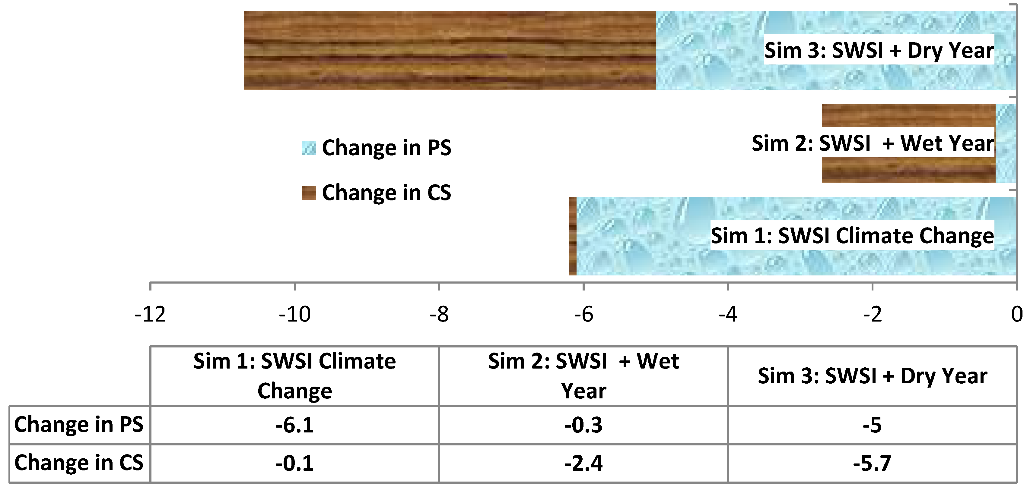
Welfare Effects. Because the model captures changes in prices and quantities, and has demand and supply functions embedded in the objective function, it is possible to determine changes in producer and consumer surpluses under the different simulations. In this fashion, the model shows how costs of climate change are borne, and could be employed to assess the value of various mitigation strategies in a future study. These results are presented in Figure 2. The measures of economic surplus show approximately a $10.7 M reduction in the S3-DRY scenario, compared to about $2.7 M in the wet year in S2-WET. In other words, the agricultural economy in Colorado loses nearly five times as much in a dry year climate relative to a wet year. The S1 climate scenario is predicted to produce economic net welfare impact that fits in the middle between S2-WET and S3-DRY (at about $6.2 M).

Figure 2. Changes in Producer Surplus (PS) and Consumer Surplus (CS), Million of Dollars.

Figure 2. Changes in Producer Surplus (PS) and Consumer Surplus (CS), Million of Dollars.

In S1, most impacts fall on producers through reduced hay area, which has the greatest effect due to its water use, and which is made up by added imports and reduced dairy production. The largest effects naturally come in the dry year simulation, where cultivated area is reduced by up to 60% for some crops and yields can decline by over 10%. The total losses in S3 of more than $10 M are split about evenly between consumers and producers. Even though prices for livestock and major crops often increase by up to 10%, the decline in quantities offsets those better prices, and there is a net loss in producer surplus, which occurs because of the openness of the agricultural economy. The consumers lose in S3-DRY due to the higher overall prices.

Conclusions

Using an Economic Displacement Mathematical Programming (EDMP) model, derived from Harrington and Dubman [34] of the USDA’s Economic Research Service. This study examines the effects of climate change on agriculture in Colorado taking into account of selected features projected several decades into the future. Initially, an overview of agriculture in the state and its dependence on water, a critical input, is described. The overview shows that the agricultural economy in Colorado is dominated by livestock, which accounts for 67% of total receipts. Crops, including feed grains and forages, account for 33% of production. Most of agriculture is based on irrigated production, which depends on both groundwater, especially from the Ogallala aquifer, and surface water that comes from runoff derived from snowpack in the Rocky Mountains. Climate studies point to decline in runoff from 6% to 20% by 2050. The timing of runoff is projected to begin and peak earlier in the spring and late-summer, and overall flows may be reduced.

The climate change scenarios evaluated in this paper include three simulations relative to a Base scenario that reflects some key characteristics with regard to future water and yield effects of climate change. Following SWSI projections, the base reflects demographics and economic changes from the calibrated model for 2007. The Base scenario models a 10.3% reduction in agricultural water from increased municipal and industrial water demand, and assumes a 75% increase in corn extracted-ethanol production. The first simulation reduces agricultural water availability by a further 14.0%, for a combined decrease of 24.3%, due to climatic factors and related groundwater depletion. The second simulation describes a year with warmer than historical average temperatures and wetter conditions, which negatively affect yields of irrigated corn and milking cows, but it improves yields for non-irrigated wheat, corn silage, irrigated hay, rangeland and pasture. In contrast, the last simulation describes a drought year, which leads to reduced harvested hectares for corn and wheat, and negatively affects yields for dry land wheat, irrigated corn, pasture and rangeland, while irrigated corn silage and hay output increase.

Three commodities examined in this paper account for a large percent of production in the Colorado agricultural sector: fed beef, wheat and dairy; two others are major sources of feed, including hay and corn. All are strongly affected by the S3-DRY scenario. Cattle feeding is dependent on exports out of the state, and in S3-DRY, fed beef production declines by 7.5% due to the significantly higher prices of feed and the resulting effect on output price. For corn, the hectares decrease by about 38% on irrigated land in both regions, while in the Arkansas basin, non-irrigated land declines by 75%. Due to the dry year’s conditions, nearly a 50% reduction of South Platte non-irrigated wheat area occurs, while the Arkansas River basin non-irrigated wheat disappears completely. The wheat crop is extremely sensitive to how rainfall is affected by climate change, with the variation in exports being nearly 1.5 M tons.

The dairy sector reacts strongly to climate variation, given that production decreases by 18% in both warmer scenarios. Dairy is the second largest user of hay, after cow calf producers, and it is the second largest user of grain, after cattle feeding, as its rations require more of each basic feedstuff. Therefore, as feed shortages develop, dairy declines first and frees up significant proportions of grain and forage. The reduction in corn area leaves irrigated land available for hay production in the Arkansas basin, and expansion in irrigated hay occurs in the same basin in drought scenario. In the South Platte, non-irrigated corn becomes competitive on the land that was previously in wheat. Notably, 280 k hectares are in hay production in other parts of Colorado throughout all simulations because excess water relative to land exists in that part of the state.

This model has not taken into account farmers’ adaptation strategies, which would reduce the climate impact on yields. Such strategies might include changing planting schedules, production practices or technologies, and the introduction of drought-tolerant varieties. Also, the model has not reflected climate-induced shifts in planting decisions and production practices that lead to various environmental impacts and higher costs. There could be soil and water quality effects through nutrient loss and soil erosion, and a greater use of pesticides to combat a higher prevalence of pests.

These environmental dimensions can be fruitful areas to examine in future research, as would be the development of a wider range of conditions in the analysis of climate change effects in the future. Some of the latter areas could be to look at various productivity growth scenarios before adding the effects of climate change, and also broader alternatives in performance of different commodities. This paper assumes certain large effects, such as the increase in yields for hay and the decrease in dairy output, but others, such as using the current set of relative prices and import and export positions as starting points, may seem to understate the climate change impacts on the agricultural economy of Colorado. A more extensive examination of these settings could provide additional insights.