Integrated River and Coastal Hydrodynamic Flood Risk Mapping of the LaHave River Estuary and Town of Bridgewater, Nova Scotia, Canada

Abstract
:1. Introduction
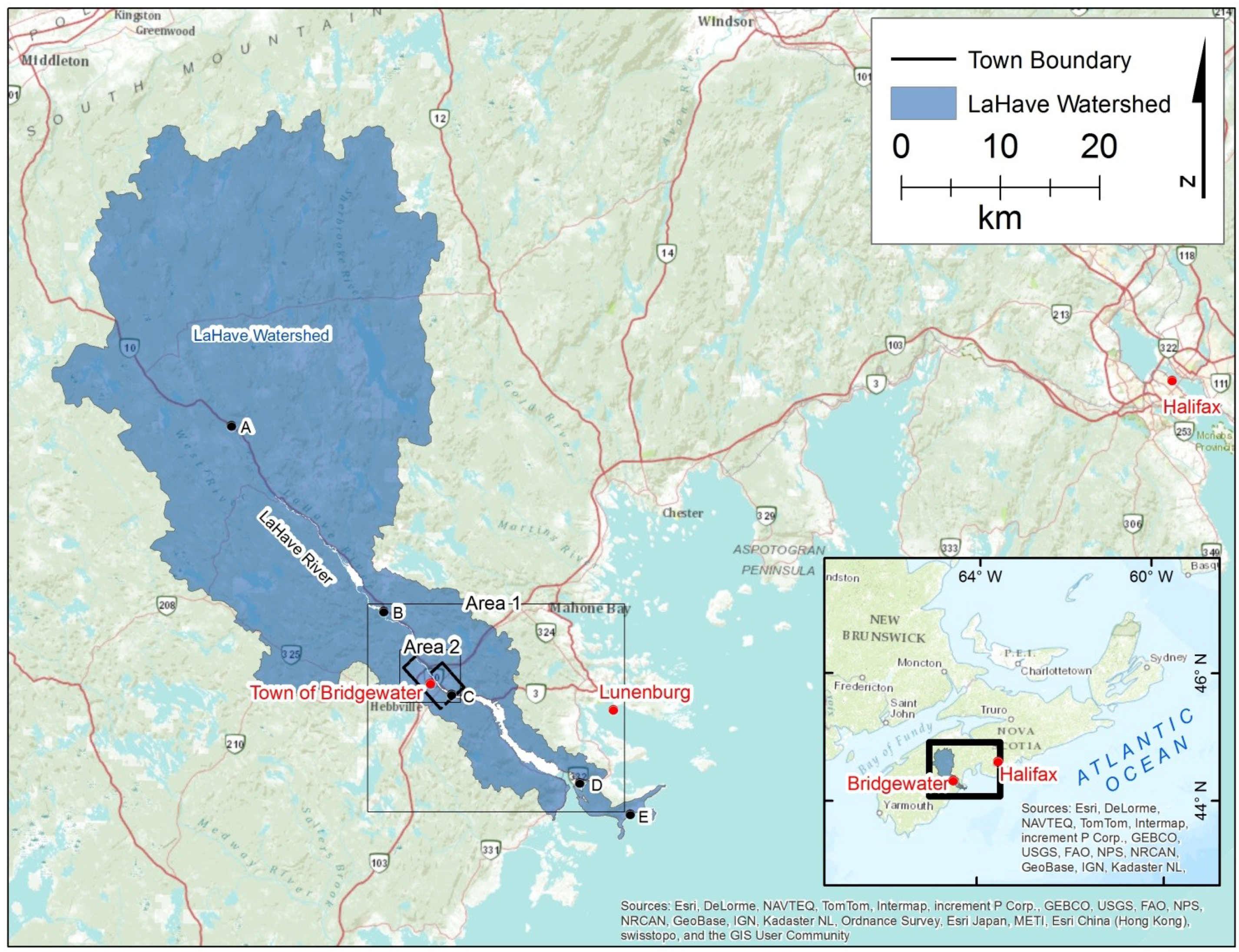
1.1. Study Area
1.2. Coastal Flooding
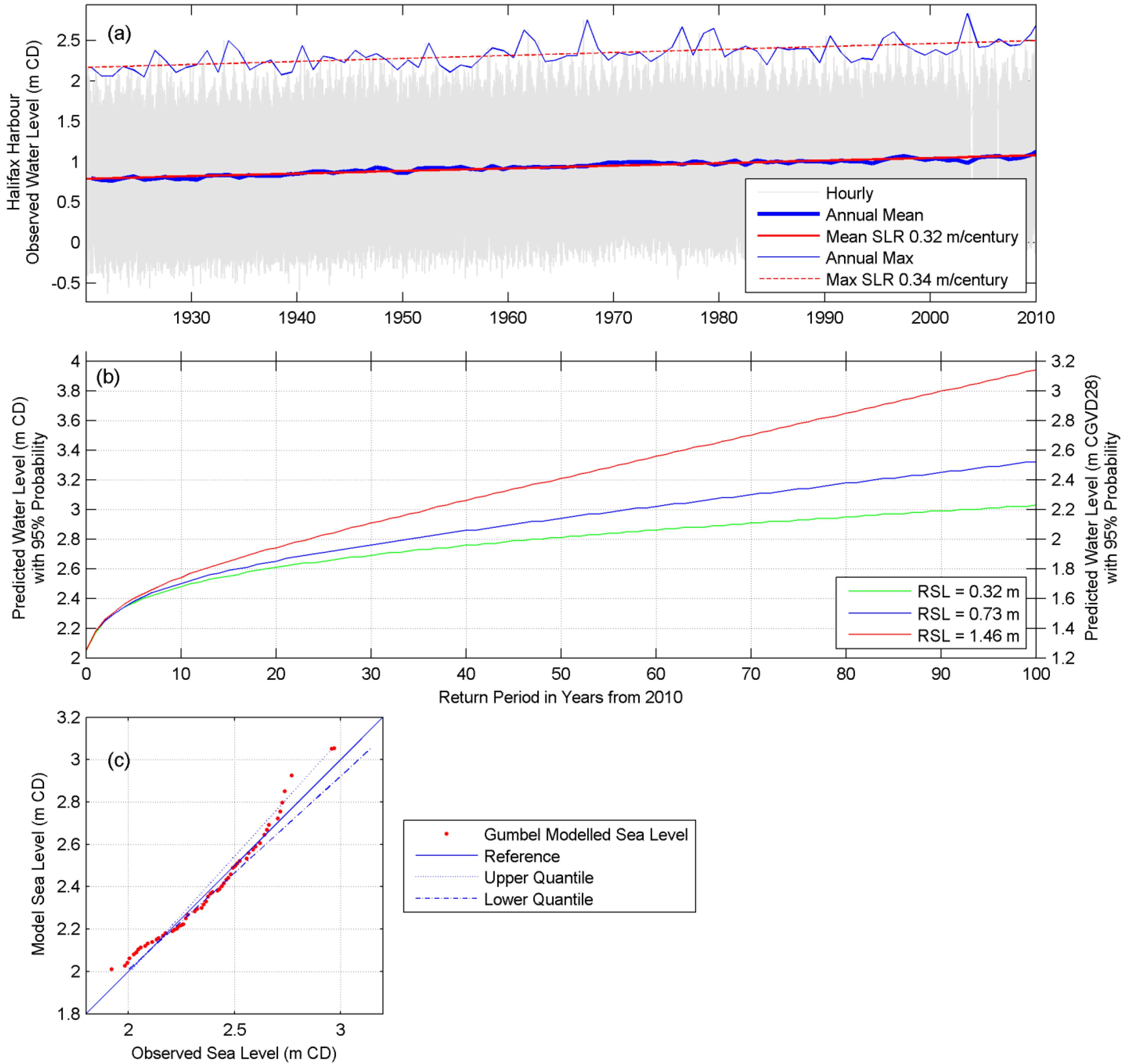
1.3. Sea-Level Rise and Climate Change

| Extreme Total Sea Level [meters Chart Datum (CD)]—Lunenburg | ||||||
|---|---|---|---|---|---|---|
| Return Period | Residual | Level 2000 | Level 2025 | Level 2055 | Level 2085 | Level 2100 |
| 10 Years | 0.71 ± 0.20 | 3.14 ± 0.20 | 3.29 ± 0.23 | 3.57 ± 0.35 | 3.97 ± 0.56 | 4.20 ± 0.68 |
| 25 Years | 0.81 ± 0.20 | 3.24 ± 0.20 | 3.39 ± 0.23 | 3.67 ± 0.35 | 4.07 ± 0.56 | 4.30 ± 0.68 |
| 50 Years | 0.88 ± 0.20 | 3.31 ± 0.20 | 3.46 ± 0.23 | 3.73 ± 0.35 | 4.14 ± 0.56 | 4.37 ± 0.68 |
| 100 Years | 0.95 ± 0.20 | 3.38 ± 0.20 | 3.53 ± 0.23 | 3.80 ± 0.35 | 4.21 ± 0.56 | 4.44 ± 0.68 |
1.4. Fluvial Flooding
1.5. Precipitation and Climate Change
2. Methods
2.1. Hydrology Data
2.2. DEM Development
2.2.1. Bathymetric Survey
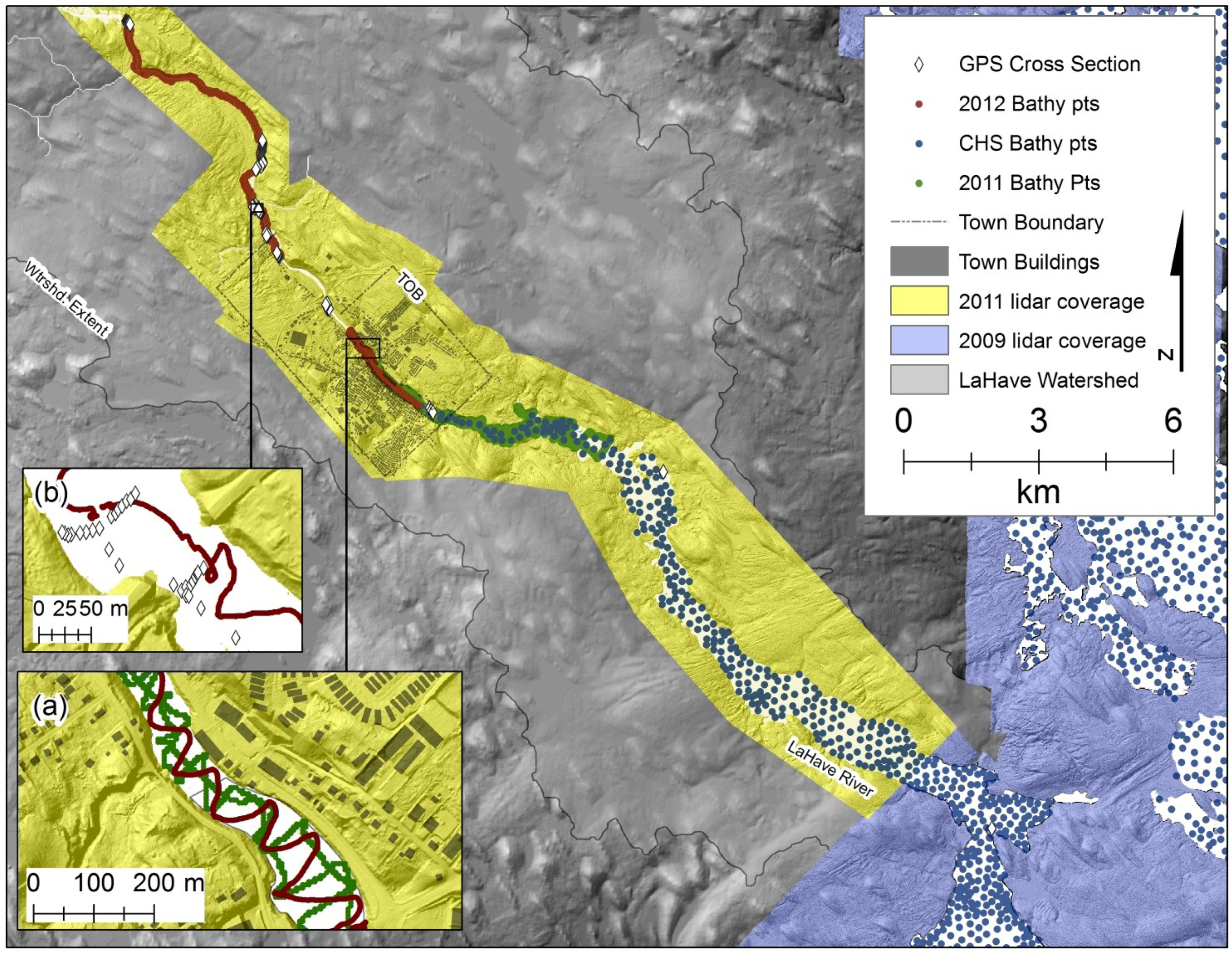
2.2.2. Lidar Survey
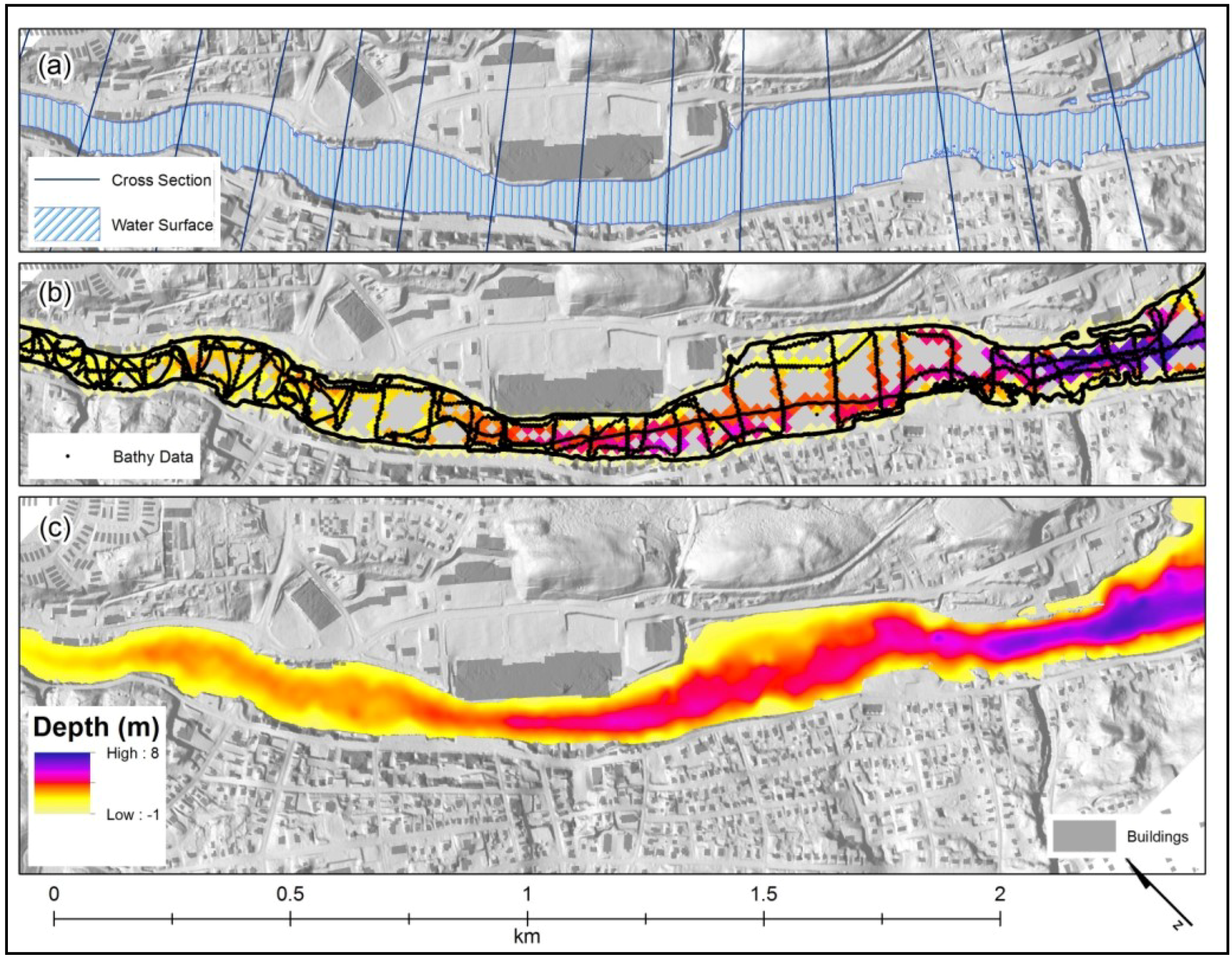
2.2.3. Lidar—Bathymetry Integration

2.3. Hydrodynamic Modeling
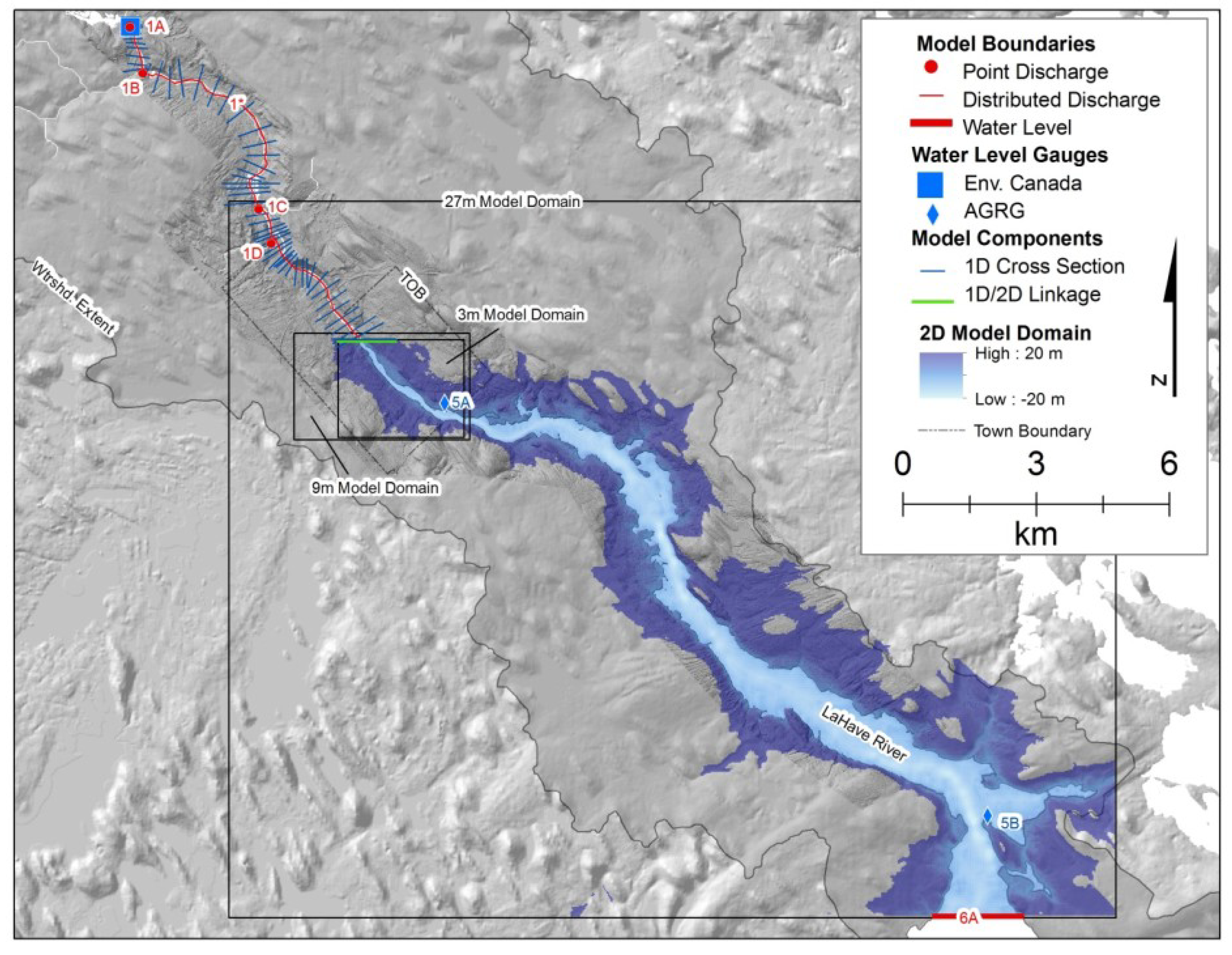
2.3.1. 1-D Model

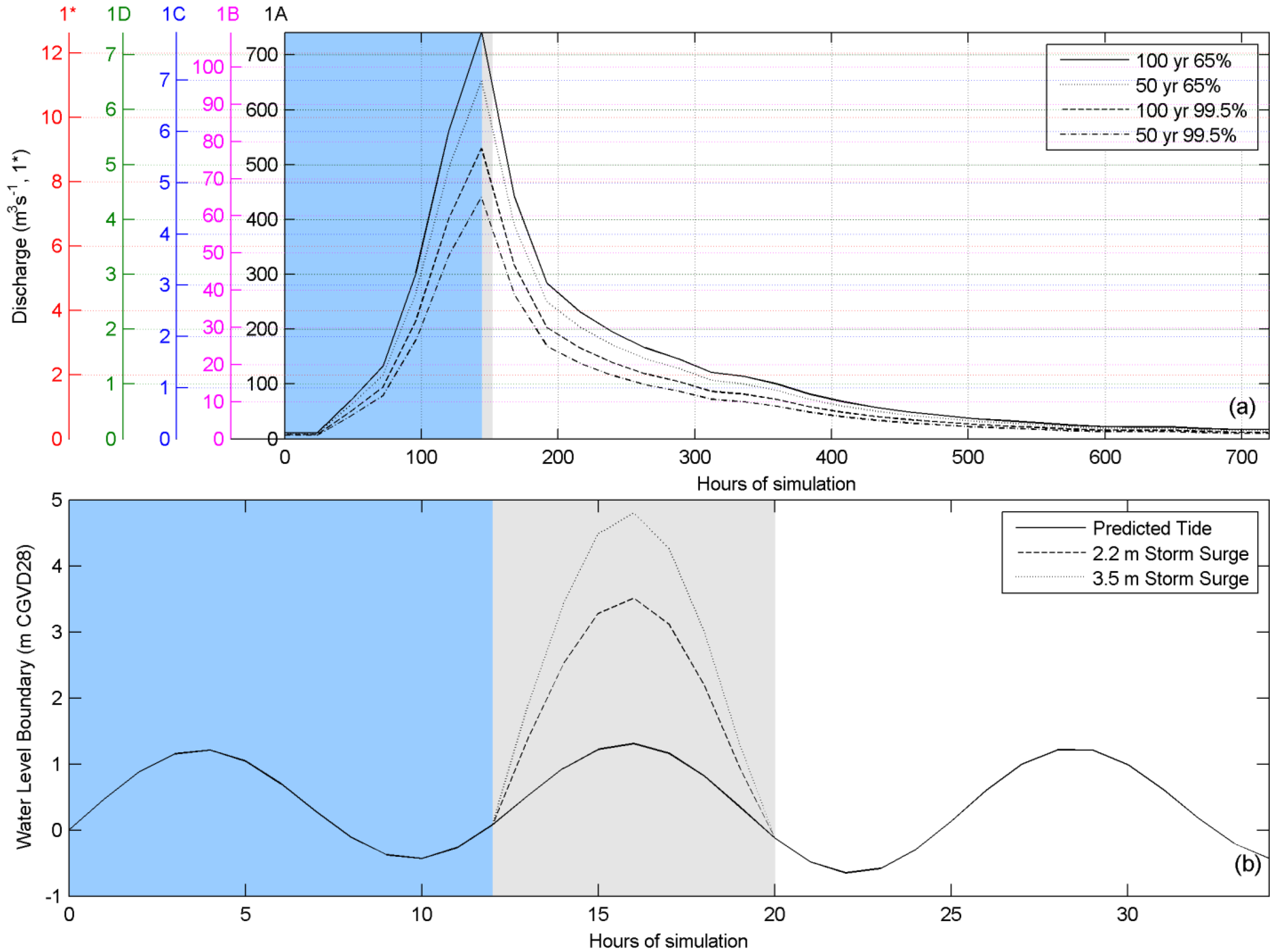
| Event Probability | Return Period in Years | Discharge (m3/s) |
|---|---|---|
| 65% | 50 | 652 |
| 65% | 100 | 741 |
| 99.5% | 50 | 441 |
| 99.5% | 100 | 530 |
2.3.2. 2-D Model
2.4. Model Simulations
| LaHave River | Tidal Condition | ||||
|---|---|---|---|---|---|
| Probability | Scenario | Discharge (m3/s) | Mean High | Mean High + 2.2 m | Mean High + 3.5 m |
| 99.5% | 50 year | 441 | 50,990 | 50,992 | 50,993 |
| 100 year | 530 | 100,990 | 100,992 | 100,993 | |
| 65% | 50 year | 652 | 50,650 | 50,652 | 50,653 |
| 100 year | 741 | 100,650 | 100,652 | 100,653 | |
3. Results
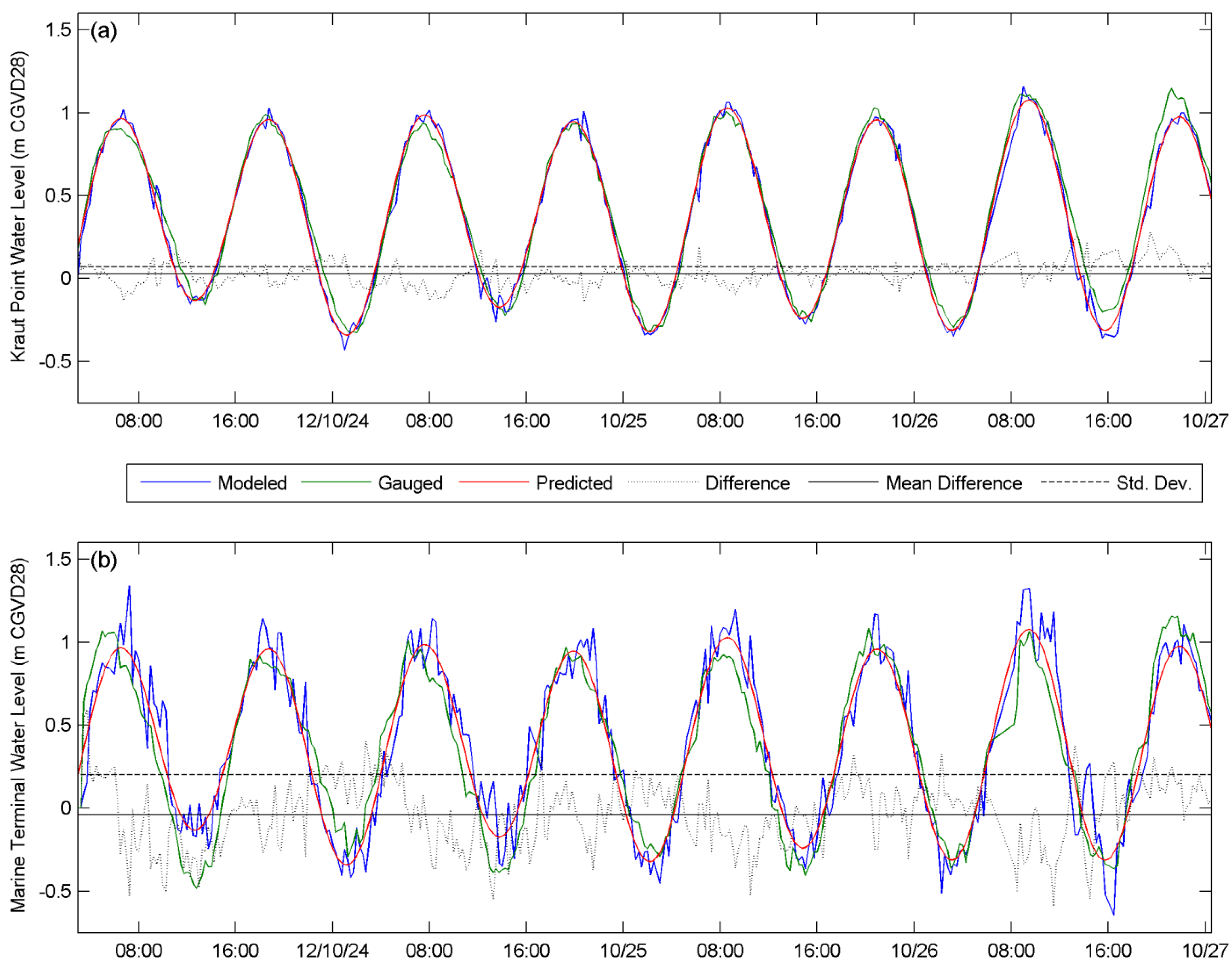
3.1. Model Validation

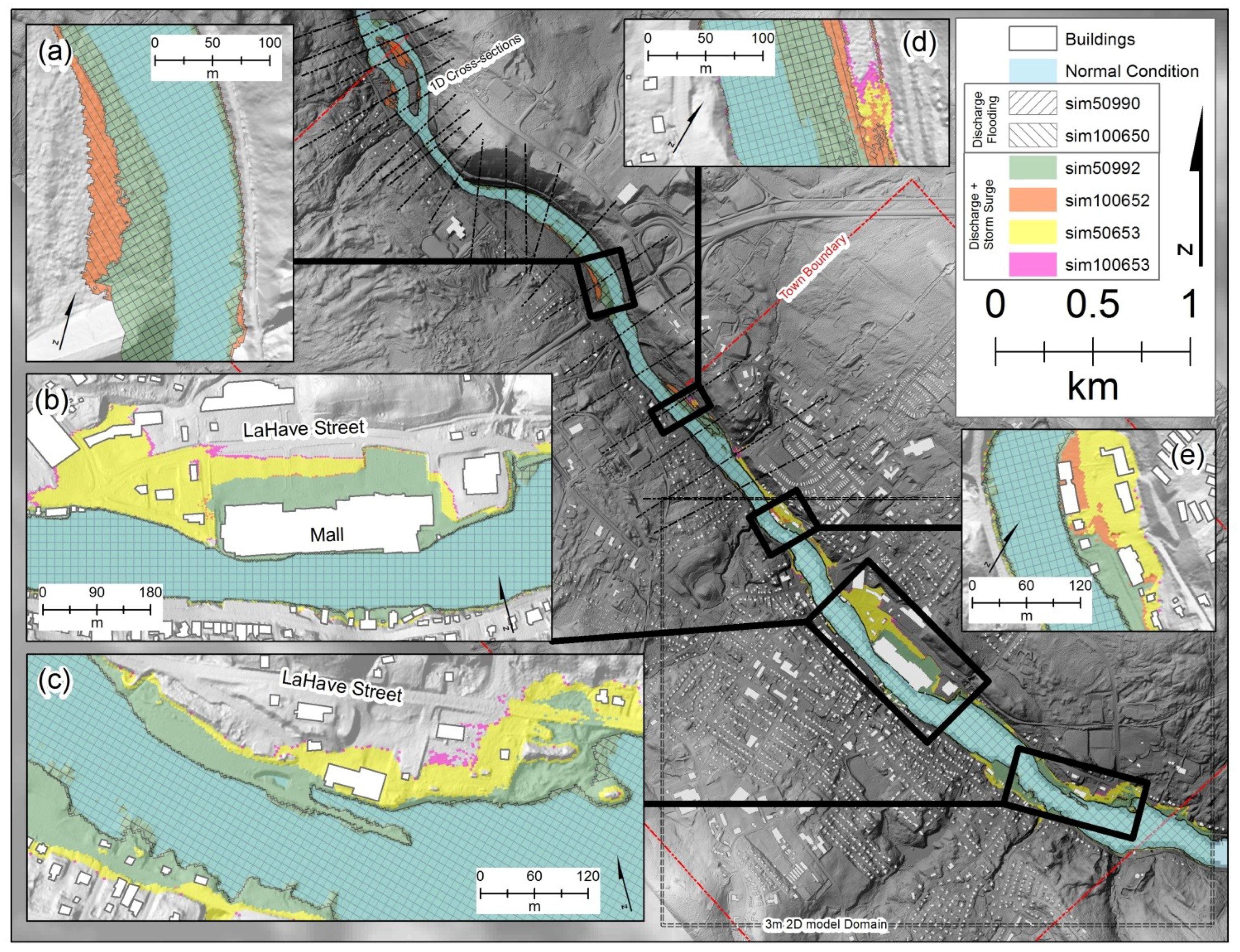
3.2. Model Simulation Results

3.3. Discussion
3.3.1. Lidar-Bathymetry DEM
3.3.2. Coupled 1-D/2-D Model

3.3.3. Return Periods of Flow
| Event | Return Period in Years | Discharge (m3/s) | Return Period (2080) |
|---|---|---|---|
| 65% probability | 50 | 652 | 47 |
| 65% probability | 100 | 741 | 88 |
| 99.5% probability | 50 | 441 | 47 |
| 99.5% probability | 100 | 530 | 88 |
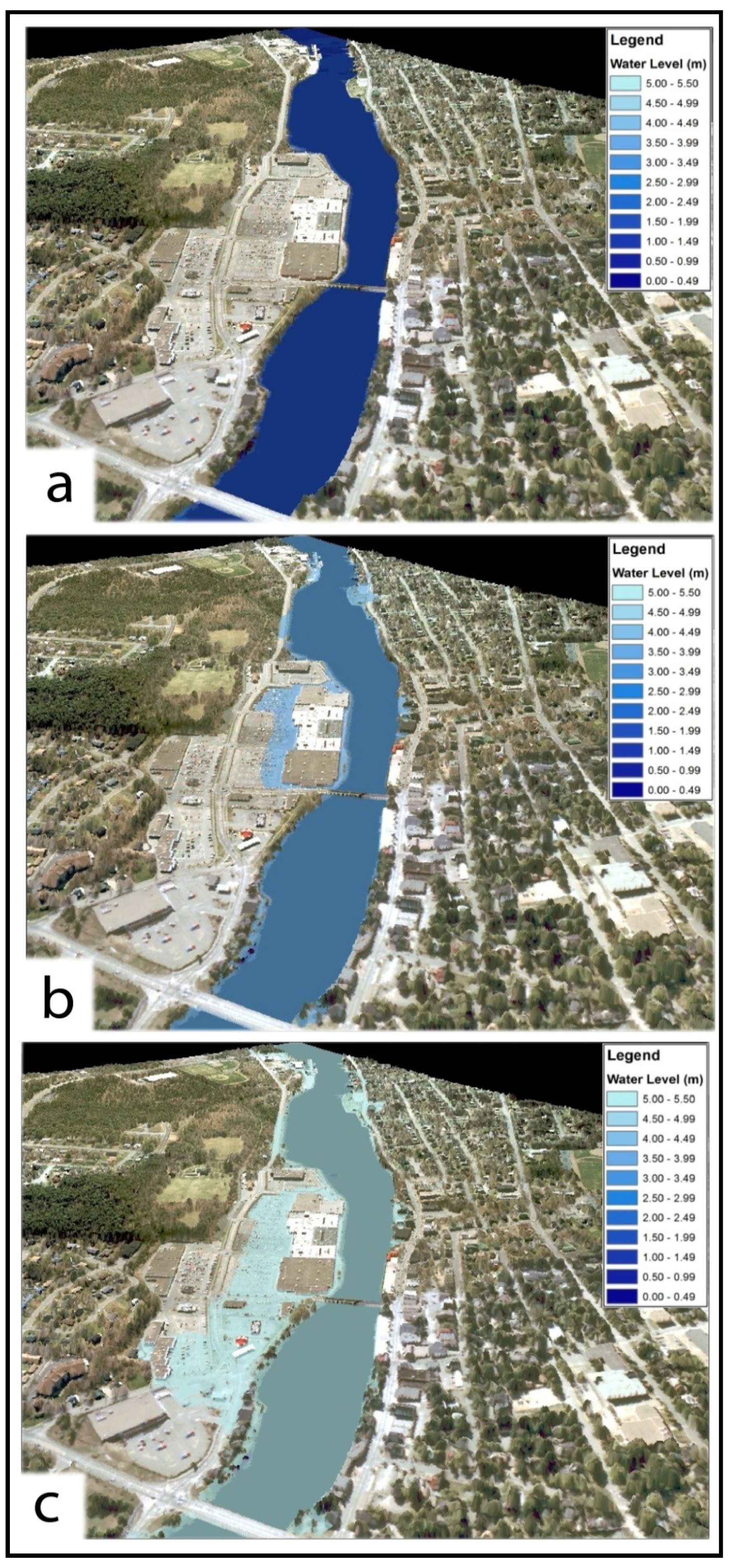
3.3.4. Maximum Flood Extent Mosaics
3.3.5. Study Limitations
4. Conclusions
Acknowledgments
Conflicts of Interest
References
- Webster, T.; McGuigan, K.; MacDonald, C. LiDAR Processing and Flood Risk Mapping for Coastal Areas in the District of Lunenburg, Town and District of Yarmouth, Amherst, County Cumberland, Wolfville and Windsor; Atlantic Climate Adaptation Solutions Association: Halifax, Canada, 2011; p. 130. [Google Scholar]
- Webster, T.; Crowell, N.; McGuigan, K.; Collins, K. Integrated River and Coastal Hydrodynamic Flood Risk Mapping; Atlantic Climate Adaptation Solutions Association: Halifax, Canada, 2012; p. 43. [Google Scholar]
- Webster, T.; McGuigan, K.; Crowell, N.; Collins, K. River Flood Risk Study of the Nappan River Incorporating Climate Change; Atlantic Climate Adaptation Solutions Association: Halifax, Canada, 2012; p. 48. [Google Scholar]
- Webster, T.; Smith, T.; Collins, K. Inventory of Physical Wastewater Infrastructure at Risk of Flooding to Climate Change induced Sea-level Incursions in the Minas Basin Area; Atlantic Climate Adaptation Solutions Association: Halifax, Canada, 2012. [Google Scholar]
- Haile, A.T.; Rientjes, T.H.M. Effects of Lidar DEM resolution in flood modelling: A model sensitivity study for the city of Tegucigalpa, Honduras. In Proceedings of ISPRS WG III/3, III/4, V/3 Workshop “Laser scanning 2005”, Enschedethe Netherlands, 12–14, September, 2005; pp. 168–173.
- Mason, D.C.; Horritt, M.S.; Hunter, N.M.; Bates, P.D. Use of fused airborne scanning laser altimetry and digital map data for urban flood modelling. Hydrol. Process. 2007, 21, 1436–1447. [Google Scholar] [CrossRef]
- Abdullah, A.F.; Vojinovic, Z.; Rahman, A.A. A Methodology for Processing Raw LiDAR Data to Support Urban Flood Modelling Framework: Case Study—Kuala Lumpur Malaysia. In Developments in Multidimensional Spatial Data Models; Rahman, A.A., Boguslawski, P., Gold, C., Said, M.N., Eds.; Springer: Berlin, Germany, 2013; pp. 49–68. [Google Scholar]
- Abderrezzak, K.E.K.; Paquier, A.; Mignot, E. Modelling flash flood propagation in urban areas using a two-dimensional numerical model. Nat. Hazards 2009, 50, 433–460. [Google Scholar] [CrossRef]
- Webster, T.; Forbes, D.L. Using airborne LIDAR to map exposure of coastal areas in Maritime Canada to flooding from storm-surge events: A review of recent experience. In Proceedings of Canadian Coastal Conference, Dartmouth, Canada, 6–9 November 2005.
- Poulter, B.; Halpin, P.N. Raster modelling of coastal flooding from sea-level rise. Int. J. Geogr. Inf. Sci. 2008, 22, 167–182. [Google Scholar] [CrossRef]
- Webster, T.L.; Forbes, D.L.; Dickie, S.; Shreenan, R. Using topographic lidar to map flood risk from storm-surge events for Charlottetown, Prince Edward Island, Canada. Can. J. Remote Sens. 2004, 30, 64–76. [Google Scholar] [CrossRef]
- Webster, T.L.; Forbes, D.L. Airborne Laser Altimetry for Predictive Modeling of Coastal Storm-Surge Flooding. In Remote Sensing of Aquatic Coastal Ecosystem Processes; Richardson, L.L., LeDrew, E.F., Eds.; Springer Netherlands: Dordrecht, the Netherlands, 2006; pp. 157–182. [Google Scholar]
- Webster, T.L.; Forbes, D.L.; MacKinnon, E.; Roberts, D. Flood-risk mapping for storm-surge events and sea-level rise using lidar for southeast New Brunswick. Can. J. Remote Sens. 2006, 32, 194–211. [Google Scholar] [CrossRef]
- Smith, R.A.E.; Bates, P.D.; Hayes, C. Evaluation of a coastal flood inundation model using hard and soft data. Environ. Model. Softw. 2012, 30, 35–46. [Google Scholar]
- Cin, C.D.; Moens, L.; Dierickx, P.; Bastin, G.; Zech, Y. An integrated approach for realtime floodmap forecasting on the Belgian Meuse River. Nat. Hazards 2005, 36, 237–256. [Google Scholar] [CrossRef]
- Moore, M.R. Development of a High-Resolution 1D/2D Coupled Flood Simulation of Charles City, Iowa. Master’s Thesis, University of Iowa, 2011. Available online: http://ir.uiowa.edu/cgi/viewcontent.cgi?article=2417&context=etd (accessed on 12 March 2014). [Google Scholar]
- Casas, A.; Benito, G.; Thorndycraft, V.R.; Rico, M. The topographic data source of digital terrain models as a key element in the accuracy of hydraulic flood modelling. Earth Surf. Process. Landforms 2006, 31, 444–456. [Google Scholar] [CrossRef]
- Cook, A.; Merwade, V. Effect of topographic data, geometric configuration and modeling approach on flood inundation mapping. J. Hydrol. 2009, 377, 131–142. [Google Scholar] [CrossRef]
- Horritt, M.S.; Bates, P.D. Evaluation of 1D and 2D numerical models for predicting river flood inundation. J. Hydrol. 2002, 268, 87–99. [Google Scholar] [CrossRef]
- Brown, J.D.; Spencer, T.; Moeller, I. Modeling storm surge flooding of an urban area with particular reference to modeling uncertainties: A case study of Canvey Island, United Kingdom: Modeling storm surge flooding of an urban area. Water Resour. Res. 2007, 43, 1–22. [Google Scholar]
- Gouldby, B.; Sayers, P.; Mulet-Marti, J.; Hassan, M.A.A.M.; Benwell, D. A methodology for regional-scale flood risk assessment. Proc. ICE Water Manag. 2008, 161, 169–182. [Google Scholar]
- Webster, T.; Sangster, C.; Kingston, D.; Christian, M. High-Resolution Elevation and Image Data within the Bay of Fundy Coastal Zone, Nova Scotia, Canada. In GIS for Coastal Zone Management; Smith, J., Darius Bartlett, E., Eds.; CRC Press: Boca Raton, FL, USA, 2004. [Google Scholar]
- Gilles, D.; Young, N.; Schroeder, H.; Piotrowski, J.; Chang, Y.-J. Inundation mapping initiatives of the Iowa Flood Center: Statewide coverage and detailed urban flooding analysis. Water 2012, 4, 85–106. [Google Scholar] [CrossRef]
- Patro, S.; Chatterjee, C.; Mohanty, S.; Singh, R.; Raghuwanshi, N.S. Flood inundation modeling using Mike Flood and remote sensing data. J. Indian Soc. Remote Sens. 2009, 37, 107–118. [Google Scholar] [CrossRef]
- Sto. Domingo, N.D.; Paludan, B.; Madsen, H.; Hansen, F.; Mark, O. Climate Change and Storm Surges: Assessing Impacts on Your Coastal City Through Mike Flood Modeling; Danish Hydraulic Institute Group: Copenhagen, Denmark, 2010; p. 11. [Google Scholar]
- Neily, P.D.; Quigley, E.; Benjamin, L.; Stewart, B.; Duke, T. Ecological Land Classification for Nova Scotia Volume 1—Mapping Nova Scotia’s Terrestrial Ecosystems; Nova Scotia Department of Natural Resources Renewable Resources Branch: Halifax, Canada, 2003; p. 83. [Google Scholar]
- Government of Canada; Environment Canada; Weather and Meteorology. Canadian Hurricane Centre—FAQ. Available online: http://www.ec.gc.ca/ouragans-hurricanes/default.asp?lang=En&n=3F0FD4CF-1#ws3C219DFF (accessed on 6 November 2013).
- Taylor, R.B.; Frobel, D.; Forbes, D.L.; Mercer, D. Impacts of Post-tropical Storm Noel (November, 2007) on the Atlantic Coastline of Nova Scotia; Geological Survey of Canada: Dartmouth, Canada, 2008. [Google Scholar]
- Hurricane Bill. Available online: http://past.theweathernetwork.com/your_weather/details/786/1442612/bridgewater/hits/1#utmxid=EAAAACD_N29-7CmDyYe4sM7ENrk;utmxpreview=0 (accessed on 12 March 2014).
- IPCC. Summary for Policymakers. In Climate Change 2013: The Physical Science Basis; Contribution of Working Group I to the Fifth Assessment Report of the Intergovernmental Panel on Climate Change; Stocker, T.F., Qin, D., Plattner, G.-K., Tignor, M., Allen, S.K., Boschung, J., Nauels, A., Xia, Y., Bex, V., Midgley, P.M., Eds.; Cambridge University Press: Cambridge, UK, 2013. [Google Scholar]
- Raper, S.C.B.; Braithwaite, R.J. Low sea level rise projections from mountain glaciers and icecaps under global warming. Nature 2006, 439, 311–313. [Google Scholar] [CrossRef]
- Church, J.A.; Gregory, J.M.; Huybrechts, P.; Kuhn, M.; Lambeck, K.; Nhuan, D.; Qin, D.; Woodworth, P.L. Changes in Sea Level. In Climate Change 2001: The Scientific Basis; Contribution of Working Group I to the Third Assessment Report of the Intergovernmental Panel; Douglas, B.C., Ramirez, A., Eds.; Cambridge University Press: Cambridge, UK, 2001. [Google Scholar]
- Meehl, G.A.; Stocker, T.F.; Collins, W.D.; Friedlingstein, P.; Gaye, A.T.; Gregory, J.M.; Kitoh, A.; Knutti, R.; Murphy, J.M.; Noda, A.; et al. Global Climate Projections. In Climate Change 2007: The Physical Science Basis; Contribution of Working Group I to the Fourth Assessment Report of the Intergovernmental Panel on Climate Change; Solomon, S., Qin, D., Manning, M., Chen, Z., Marquis, M., Averyt, K.B., Tignor, M., Miller, H.L., Eds.; Cambridge University Press: Cambridge, UK, 2007. [Google Scholar]
- Forbes, D.L.; Manson, G.K.; Charles, J.; Thompson, K.R.; Taylor, R.B. Halifax Harbour Extreme Water Levels in the Context of Climate Change: Scenarios for a 100-Year Planning Horizon; Natural Resources Canada: Ottawa, Canada, 2009; p. 22. [Google Scholar]
- Rahmstorf, S.; Cazenave, A.; Church, J.A.; Hansen, J.E.; Keeling, R.F.; Parker, D.E.; Somerville, R.C.J. Recent climate observations compared to projections. Science 2007, 316, 709–709. [Google Scholar] [CrossRef]
- Shaw, J.; Taylor, R.B.; Forbes, D.L.; Ruz, M.-H.; Solomon, S. Sensitivity of the Coasts of Canada to Sea-level Rise; Natural Resources Canada: Ottawa, Canada, 1998; pp. 1–79. [Google Scholar]
- Webster, T. Flood risk mapping using LiDAR for Annapolis Royal, Nova Scotia, Canada. Open Access Remote Sens. 2010, 2, 2060–2082. [Google Scholar] [CrossRef]
- Webster, T.; Stiff, D. The prediction and mapping of coastal flood risk associated with storm surge events and long-term sea level changes. In Risk Analysis VI Simulations and Hazard Mitigation; Brebbia, C.A., Beriatos, E., Eds.; WIT Press: Southampton, UK, 2008; pp. 129–139. [Google Scholar]
- Webster, T.; Mosher, R.; Pearson, M. Water modeler: A component of a coastal zone decision support system to generate flood-risk maps from storm surge events and sea-level rise. Geomatica 2008, 62, 393–406. [Google Scholar]
- Shaw, J.; Taylor, R.B.; Forbes, D.L.; Ruz, M.-H.; Solomon, S. Sensitivity of the Canadian Coast to Sea-Level Rise; Geological Survey of Canada: Otttawa, Canada, 1994; p. 114. [Google Scholar]
- McCulloch, M.M.; Forbes, D.L.; Shaw, R.D. Coastal Impacts of Climate Change and Sea-Level Rise on Prince Edward Island; Geological Survey of Canada: Ottawa, Canada, 2002. [Google Scholar]
- Peltier, W.R. Global glacial isotasy and the surface of the ice-age earth: The ICE-5G (VM2) model and GRACE. Annu. Rev. Earth Planet. Sci. 2004, 32, 111–149. [Google Scholar] [CrossRef]
- Knutson, T.R.; McBride, J.L.; Chan, J.; Emanuel, K.; Holland, G.; Landsea, C.; Held, I.; Kossin, J.P.; Srivastava, A.K.; Sugi, M. Tropical cyclones and climate change. Nat. Geosci. 2010, 3, 157–163. [Google Scholar] [CrossRef] [Green Version]
- Emanuel, K. Increasing destructiveness of tropical cyclones over the past 30 years. Nature 2005, 436, 686–688. [Google Scholar] [CrossRef]
- Richards, W.; Daigle, R. Scenarios and Guidance for Adaptation to Climate Change and Sea Level Rise- NS and PEI Municipalities; Atlantic Climate Adaptation Solutions Association: Halifax, Canada, 2011; p. 87. [Google Scholar]
- Bernier, N.B. Annual and Seasonal Extreme Sea Levels in the Northwest Atlantic: Hind Casts over the Last 40 Years and Projections for the Next Century. Ph.D. Thesis, Dalhousie University, Halifax, NS, USA, December 2005. [Google Scholar]
- Environment Canada. Public Alerting Criteria. Available online: http://www.ec.gc.ca/meteo-weather/default.asp?lang=En&n=D9553AB5-1#rainfall (accessed on 6 November 2013).
- Environment Canada. Causes of Flooding. Available online: http://www.ec.gc.ca/eau-water/default.asp?lang=En&n=E7EF8E56-1#snowmelt (accessed on 8 November 2013).
- Government of Canada; Environment Canada. Real-time Hydrometric Data. Available online: http://www.wateroffice.ec.gc.ca/index_e.html (accessed on 22 November 2013).
- Brown, L. Flooded LaHave Claims Two Lives. South Shore, 9 April 2003. [Google Scholar]
- Bruce, J.; Burton, I.; Martin, H.; Mills, B.; Mortsch, L. Water Sector: Vulnerability and Adaptation to Climate Change; Final Report; GCSI—Global Change Strategies International Inc. and The Meteorological Service of Canada: Ottawa, Canada, 2000. [Google Scholar]
- Mekis, E.; Hogg, W.D. Rehabilitation and analysis of Canadian daily precipitation time series. Atmosphere-Ocean 1999, 37, 53–85. [Google Scholar] [CrossRef]
- Government of Canada, Natural Resources Canada. Canada in a Changing Climate: Atlantic Canada. Available online: http://www.nrcan.gc.ca/earth-sciences/climate-change/community-adaptation/830 (accessed on 6 November 2013).
- Madsen, T.; Willcox, N. When It Rains, It Pours Global Warming and the Increase in Extreme Precipitation from 1948 to 2011; Environment America Research & Policy Center: Boston, MA, USA, 2012. [Google Scholar]
- Singh, D.; Tsiang, M.; Rajaratnam, B.; Diffenbaugh, N.S. Precipitation extremes over the continental United States in a transient, high-resolution, ensemble climate model experiment. J. Geophys. Res. Atmospheres 2013, 118, 7063–7086. [Google Scholar] [CrossRef]
- Toreti, A.; Naveau, P.; Zampieri, M.; Schindler, A.; Scoccimarro, E.; Xoplaki, E.; Dijkstra, H.A.; Gualdi, S.; Luterbacher, J. Projections of global changes in precipitation extremes from Coupled Model Intercomparison Project Phase 5 models. Geophys. Res. Lett. 2013, 40, 4887–4892. [Google Scholar] [Green Version]
- Nova Scotia Environment. Toward a Greener Future: Nova Scotia’s Climate Change Action Plan; Nova Scotia Department of Environment: Halifax, Canada, 2009. [Google Scholar]
- Whitfield, P.H.; Cannon, A.J. Recent variations in climate and hydrology in Canada. Can. Water Resour. J. 2000, 25, 19–65. [Google Scholar] [CrossRef]
- Zhang, X.; Harvey, K.D.; Hogg, W.D.; Yuzyk, T.R. Trends in Canadian streamflow. Water Resour. Res. 2001, 37, 987–998. [Google Scholar] [CrossRef]
- Najjar, R.G.; Walker, H.A.; Anderson, P.J.; Barron, E.J.; Bord, R.J.; Gibson, J.R.; Kennedy, V.S.; Knight, C.G.; Megonigal, J.P.; OConnor, R.E.; et al. The potential impacts of climate change on the mid-Atlantic coastal region. Clim. Res. 2000, 14, 219–233. [Google Scholar] [CrossRef]
- Intergovernmental Panel on Climate Change Working Group II. The Regional Impacts of Climate Change: An Assessment of Vulnerability; Cambridge University Press: Cambridge, UK, 1998. [Google Scholar]
- Danish Hydraulic Institute. MIKE 21 Flow Model Hydrodynamic Model Scientific Documentation. Danish Hydraulic Institute: Horsholm, Denmark, 2012. [Google Scholar]
- Thompson, K.R.; Bernier, N.B.; Chan, P. Extreme sea levels, coastal flooding and climate change with a focus on Atlantic Canada. Nat. Hazards 2009, 51, 139–150. [Google Scholar] [CrossRef]
- Snyder, N.P.; Whipple, K.X.; Tucker, G.E.; Merritts, D.J. Landscape response to tectonic forcing: Digital elevation model analysis of stream profiles in the Mendocino triple junction region, northern California. Geol. Soc. Am. Bull. 2000, 112, 1250–1263. [Google Scholar] [CrossRef]
- Tague, C.; Grant, G.E. A geological framework for interpreting the low-flow regimes of Cascade streams, Willamette River Basin, Oregon. Water Resour. Res. 2004, 40, W04303. [Google Scholar]
© 2014 by the authors; licensee MDPI, Basel, Switzerland. This article is an open access article distributed under the terms and conditions of the Creative Commons Attribution license (http://creativecommons.org/licenses/by/3.0/).
Share and Cite
Webster, T.; McGuigan, K.; Collins, K.; MacDonald, C. Integrated River and Coastal Hydrodynamic Flood Risk Mapping of the LaHave River Estuary and Town of Bridgewater, Nova Scotia, Canada. Water 2014, 6, 517-546. https://doi.org/10.3390/w6030517
Webster T, McGuigan K, Collins K, MacDonald C. Integrated River and Coastal Hydrodynamic Flood Risk Mapping of the LaHave River Estuary and Town of Bridgewater, Nova Scotia, Canada. Water. 2014; 6(3):517-546. https://doi.org/10.3390/w6030517
Chicago/Turabian StyleWebster, Tim, Kevin McGuigan, Kate Collins, and Candace MacDonald. 2014. "Integrated River and Coastal Hydrodynamic Flood Risk Mapping of the LaHave River Estuary and Town of Bridgewater, Nova Scotia, Canada" Water 6, no. 3: 517-546. https://doi.org/10.3390/w6030517