1. Introduction
1.1. Background
Gated tunnels in dams can be used for various purposes, such as regulating the surface of reservoir water, drawdown of the reservoir, sediment flushing, and flood release [
1]. For most dams, flow regulation can be performed from a low level outlet consisting of a closed conduit with a slide gate or valve. Outlet works are devices used to release and regulate water flow from a dam usually for irrigational purposes. Such devices may consist of one or more pipes or tunnels through the embankment of the dam, directing water, often under high pressure, to the river downstream [
2]. When the outlet gate is placed inside the conduit, reduced pressure, which may causes cavitation, is often measured just downstream of the gate.
Diffusing air into the flow can eliminate cavitation damages. Aeration will also improve the mean pressure and reduce the intensity of hydrodynamic pressure fluctuations [
3]. Therefore, to minimize these effects, aerators are recommended just downstream of gates to introduce air into the flow [
4].
A proper size for the air-vent pipe should be considered to allow for the sufficient amount of air flow rate. The air flow rate
Qa refers to the amount of air drawn into the air vent. Air flow can be diffused into the water flow through turbulent mixing. The process of air and water mixing can be applied by utilizing a separate air phase above the water surface of the pipe outlet [
4].
Insufficient research has been conducted on the air and water flow properties of high-velocity waters discharging at the downstream end of tunnels. Kalinske and Robertson [
5] were one of the first researchers who have studied the air demand in closed conduits as a function of the Froude number. Other researchers proposed related but alternative methods for predicting air demand discharge [
6,
7,
8,
9,
10,
11].
1.2. Purpose, Rationale, Objectives, and Boundary Conditions
The purpose of this study is to apply an adaptive network-based model for air demand estimations regarding low-level outlet works. This work also aims to determine if the use of artificial neural networks (ANN) and simpler models, such as multiple regression models for air demand estimations, could be justified.
In this study, a fuzzy rule-based model was developed for estimating air flow rate in two stages. In the first stage, local sub-regions were determined by analysing the pattern of input data. The regions can be determined intuitively, requiring often too many trial and error attempts. Therefore, alternative clustering techniques were used in this study to find the sub-sets of an input space that characterized possible occurrences of the data. In the second stage, a local model was built for each cluster. The Mamdani’s model, the Takagi–Sugeno’s (TS) model, and the standard additive model can be applied at this stage. In this study, the TS model was chosen, because it can solve complex and high-dimensional problems relying only on a few rules.
In general, artificial intelligence models such as an adaptive neuro-fuzzy inference system (ANFIS) and ANN do not need any
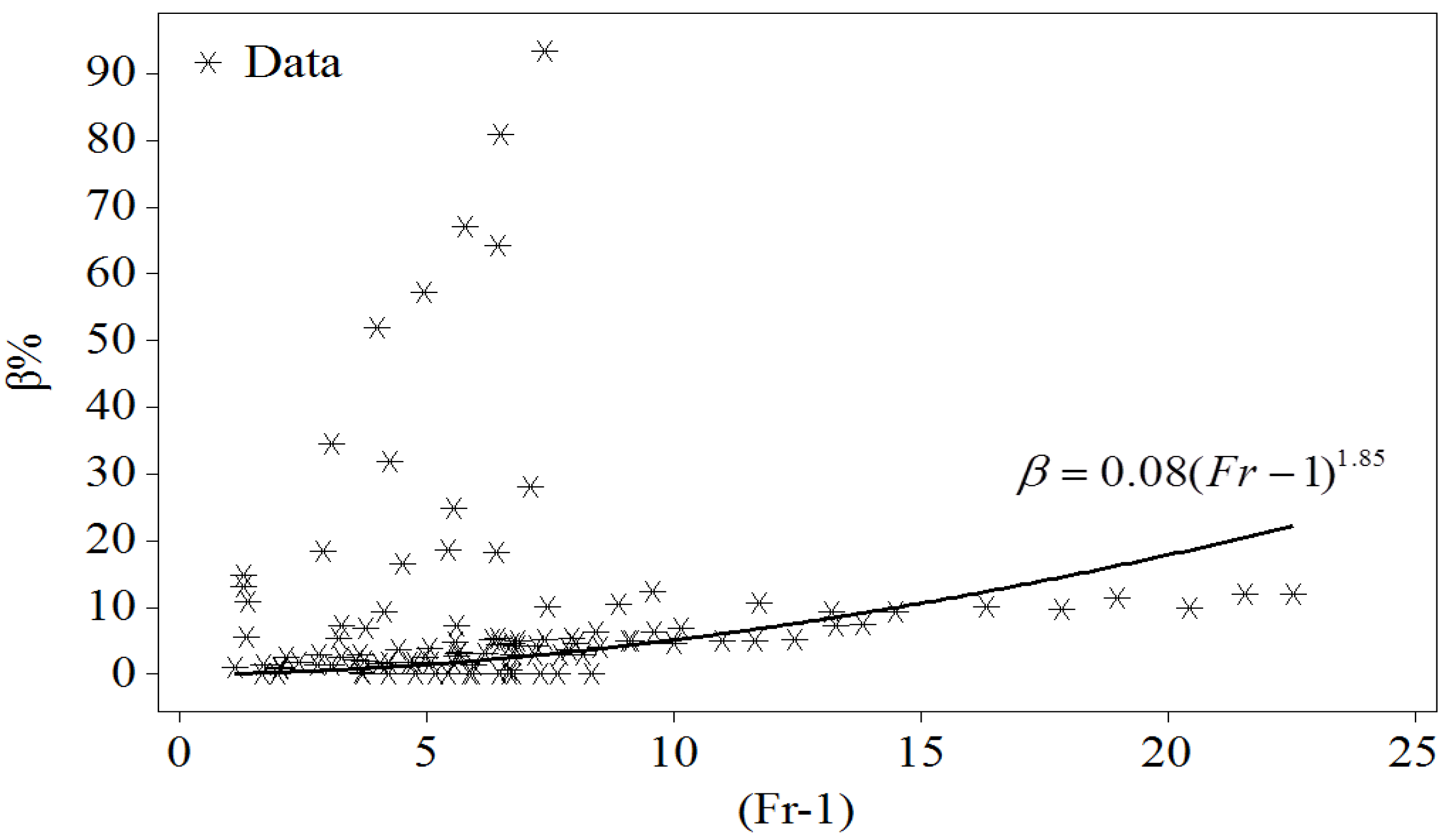
a priori assumptions to be made on the nature (linear or non-linear) of the relationship between the response variable and explanatory variables. However, the successful application of artificial intelligence in modelling requires good comprehension of the effect of some internal parameters related to the input variables, model structure, training steps, and decision-making process. The dam geometries considered in this research involved a slide gate installed on the sloping upstream face of an embankment dam, followed by a vertical elbow where the flow entered the conduit, as shown in
Figure 1. The air demand varied with gate and conduit geometry, gate opening, and water discharge passing through the gate. Hence, these parameters were considered potential input variables for the ANFIS, ANN, and multiple regression models.
Figure 1.
Typical representation of a low-level outlet works.
Figure 1.
Typical representation of a low-level outlet works.
2. Materials and Methods
2.1. Experimental Data
The 108 data used in this study were obtained from a study published by Tullis and Larchar [
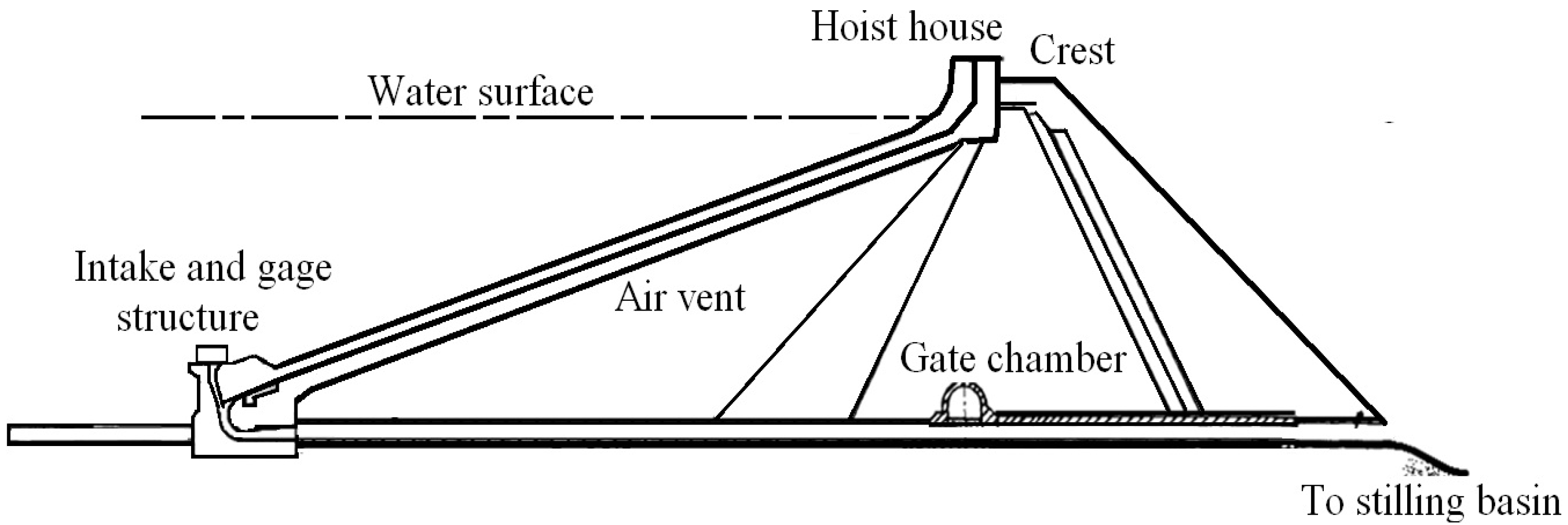
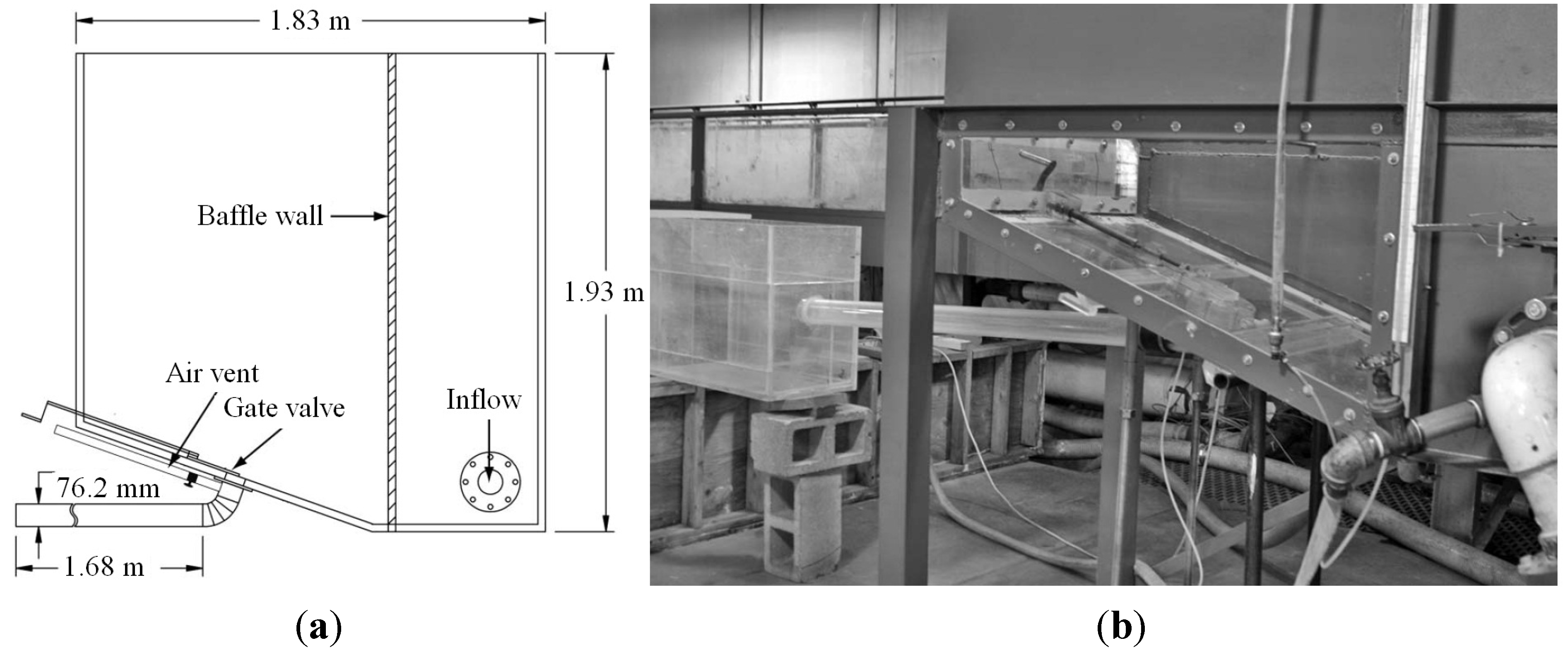
4]. In an effort to develop a better understanding of head-discharge relationships and air-venting requirements for inclined slide gates, a laboratory-scale model (
Figure 2) of low-level outlet works representative of small- to medium-sized embankment dam applications was constructed at the Utah Water Research Laboratory, Utah State University. A schematic representation of the experimental set-up is shown in
Figure 2b. The model shown in
Figure 2a consisted of an elevated steel tank (approximately 1.8 m long, 1.8 m tall and 0.9 m wide). Two acrylic slide gates (round and rectangular) were constructed and subsequently tested. The gate designs were based on commercially available slide gates. The data collected for each test condition included the area of gate (
A), opening percentage (
O%), head of water (
H), and water discharge (
Qw) for outlet conditions and the air velocity (
Va) in the supply line (vented only).
Table 1.
Design parameters after [
4].
Table 1.
Design parameters after [4].
| Extremes | Area (cm2) | Gate Opening (%) | Head (cm) | Water Discharge (L/s) | Air Discharge (L/s) |
|---|
| Minimum | 45.6 (round gate) | 10 | 13.8 | 0.3 | 0.0 |
| Maximum | 58.1 (rectangular gate) | 100 | 168.5 | 25.3 | 7.3 |
In the experiment, three different flow conditions at the downstream end of the discharge pipe were considered: (1) non-vented flow; (2) vented flow with a free-discharging pipe outlet; and (3) vented flow with a submerged pipe outlet [
4]. The data were collected at 10%, 30%, 50%, 60%, 70%, 90%, and 100% gate openings. A gate opening value represents the proportion (%) of the total linear travel distance of the gate.
Table 1 summarizes the minimum and maximum design parameters.
Figure 2.
(
a) Schematic of lab-scale low-level outlet works; and (
b) experimental set-up after [
4].
Figure 2.
(
a) Schematic of lab-scale low-level outlet works; and (
b) experimental set-up after [
4].
2.2. Empirical Relationships for Estimating Discharge Air Vents
Research has traditionally concentrated on the flow aeration downstream of bottom outlet gates. Studies are usually based on experimental information obtained from physical models. Most of the published air-venting studies are limited to large-dam outlet geometries [
4]. In order to validate the experimental relationships for low-level outlets, formulas related to large dam outlets were considered for determining the air demand in this study.
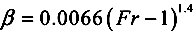
The Froude Number is a dimensionless parameter defined as the ratio of a characteristic velocity to a gravitational wave velocity [Equation (1)]. Kalinske and Robertson [
5] reported results on air demand for situations where a hydraulic jump was formed in the downstream conduit. Based on their results, the aeration coefficient (
β) for the condition of a hydraulic jump was suggested as a function of the Froude number (
Fr) as shown in Equation (2).
where
Fr is the Froude number;
V is the mean velocity of water;
Yc is the flow depth at the contracted section; and
g is the gravitational acceleration.
The aeration coefficient (
β) can also be expressed as the vent air discharge over the water flow discharge (
β = Qa/Qw). Campbell and Guyton [
6] presented Equation (3) for the air demand ratio using the Froude number in the contracted section downstream of the gate [
12].
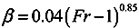
The U.S. Army Corps of Engineers [
7] published Equation (4), which is based on prototype observations. Equation (4) is rather similar to Equation (3).
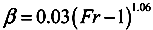
In another experiment, Sharma [
10] verified prototype data and compared results with the empirical equations in the water flow of conduits. Equation (5) directly relates the aeration coefficient to the Froude number according to Sharma’s experiments.
2.3. Adaptive Network-Based Fuzzy Inference System
The ANFIS integrates the features of fuzzy systems and neural networks. Thereafter, it has the potential to capture the benefits of both in a single framework. Membership functions are the central concept of fuzzy set theory, which numerically represents the degree to which a given element belongs to a fuzzy set [
13].
In order to avoid over-fitting of the ANFIS model, an early stopping technique has been applied. In this method, the validation set can be used to detect the time in which over-fitting starts during the supervised training. At this stage, training is stopped before convergence to avoid over-fitting [
14].
2.4. Takagi–Sugeno’s Model
The TS model was published by Takagi and Sugeno in 1985 [
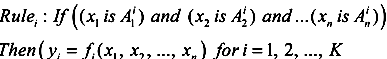
15]. A TS fuzzy model consists of four major elements of member functions, internal functions, rules, and outputs [
16]. The TS fuzzy models are quasi-linear in nature, resulting in smooth transitions between linear sub-models [
17].
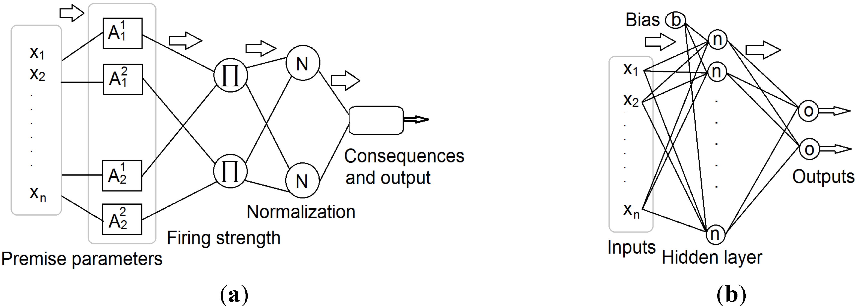
Figure 3a illustrates the typical structure of the ANFIS model. For a multi-input and single-output model, the typical fuzzy rule of a TS model is shown in Equation (6).
Figure 3.
Schematic representation of the (a) adaptive neural-based fuzzy inference system; and the (b) feed-forward Levenberg-Marquardt artificial neural network structure.
Figure 3.
Schematic representation of the (a) adaptive neural-based fuzzy inference system; and the (b) feed-forward Levenberg-Marquardt artificial neural network structure.
where
xn is the input variable,
![Water 05 01441 i011]()
is the membership function (MF) and
K is the number of fuzzy if-then rules. The consequent part of the rule base shows the rule output. In a TS fuzzy model, rule consequents are usually taken to be either crisp numbers or linear functions of the input parameters [Equation (7); layer 1].
where
yi is the output variable, and
ai and
c are parameters of the consequent parts of the rule shown in Equation (6). The number of rules is indicated by
K, and
Ai is the antecedent fuzzy set of the
i-th rule defined by the membership function
![Water 05 01441 i013]()
(premise parameters in
Figure 3a). The degree of matching between the input parameters and rule [Equation (6)] is called the rule firing strength (
Figure 3a), which is normally defined as an and-conjunction by means of the product operator [Equation (8); layer 2].
where
xj is the
j-th input variable in the
n dimensional input data space and
![Water 05 01441 i015]()
is the membership degree of the
j-th input
xj for the
i-th rule. For the input
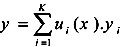
x, the total output
y of the TS model is computed by aggregating the contributions of individual rules [
17]. Therefore, the overall fuzzy system output can be obtained by Equation (9). Consequents and outputs are shown in
Figure 3a.
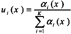
where
ui is the normalized degree of fulfilment of the antecedent clause of rule shown in Equation (6) [
13,
18]. The normalized degree of fulfilment can be expressed by Equation (10). The normalization layer is shown in
Figure 3a.
2.5. Hybrid Algorithm
Two learning methods are generally used in the adaptive TS model to specify the relationship between input and output and to determine the optimized distribution of MF. The TS model utilizes a combination of the least-square method and the back-propagation gradient descent method for training the FIS membership function parameters to identify patterns hidden in a given training dataset [
19,
20,
21,
22].
Several methods can be utilized for setting up the MF of the ANFIS (e.g., grid partition and subtractive clustering). Regarding the combination of grid partition and ANFIS, grid partition divides the input vector into a number of fuzzy regions using paralleled axis. However, in this method, fuzzy rules increase exponentially when the amount of input variables increases. Therefore, the application of grid partition in ANFIS is not recommended for large input variable problems [
23].
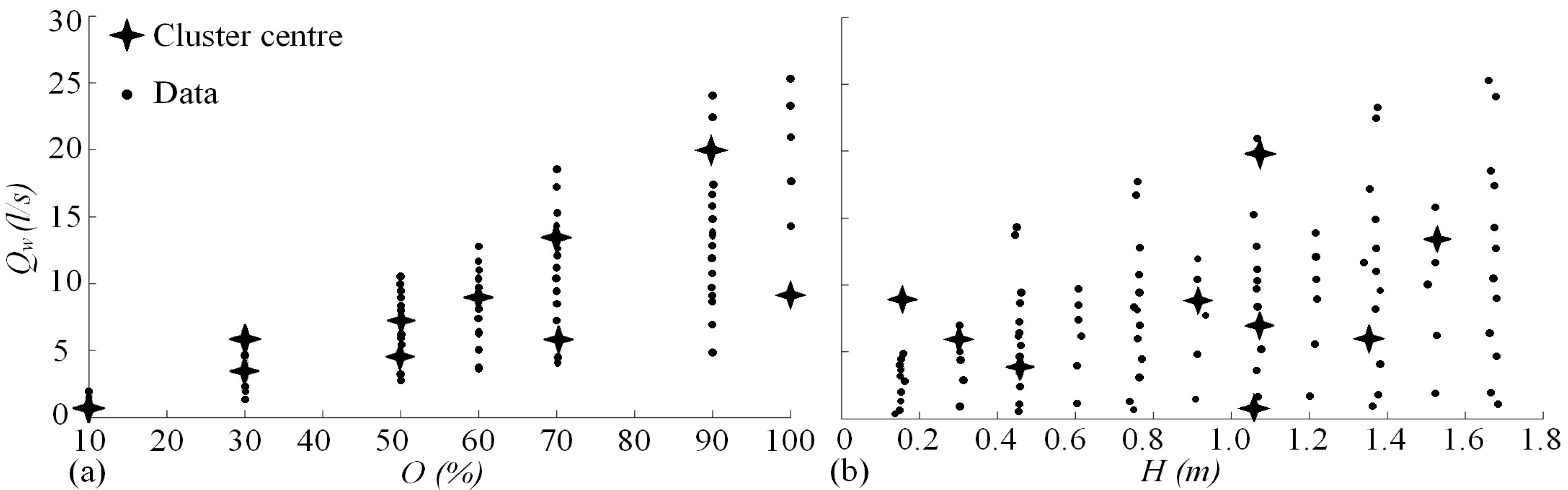
In this study, a subtractive clustering method was used to initialize the Gaussian type of MF. The simulation begins by generating the fuzzy rules using subtractive clustering, which is based on a measure of the density of data points in the feature space. This approach is applied to determine the number of rules and antecedent membership functions by considering each cluster centre as a fuzzy rule. An example of how the clusters are identified in the second (gate opening) and the fourth (water discharge) input dimensions as well as the third (head of water) and fourth (water discharge) input dimensions of the input space is shown in
Figure 4.
Figure 4.
Cluster centres using the centre of gravity method in (a) input 2 [gate opening (O)] and input 4 [water discharge (Qw)]; and in (b) input 3 [head of water (H)] and input 4 (Qw).
Figure 4.
Cluster centres using the centre of gravity method in (a) input 2 [gate opening (O)] and input 4 [water discharge (Qw)]; and in (b) input 3 [head of water (H)] and input 4 (Qw).
Desirable variables of the membership functions are optimized for the identification data set through the back-propagation procedure while a linear least squares method is used for calculating the consequent parameters. Parameters associated with membership functions change through the learning process and the gradient vector facilitates the calculation of these parameters. Each time when the gradient vector is obtained, an optimization procedure is performed to adjust parameters for reducing errors [
24].
2.8. K-fold Cross-Validation
Cross validation techniques tend to focus on not using the entire data set when building a model. They are applied for assessing how the results of statistical analysis would generalize to an independent data set. In addition, they are applied for the settings in which the goal is estimating how accurately a predictive model would perform in practice. In K-fold cross-validation, the data are split into K parts (folds) with K-1 parts as the training set and one part as the testing set.
The cross-validation process is then repeated
K times. Once the model is built using the left cases (often called the training data set), the cases that are removed (referred to as the testing data set) can be used to test the performance of the model on the ‘unseen’ data (
i.e., the testing set). The
K results from the folds can then be averaged (or otherwise combined) to produce a single estimation [
31].
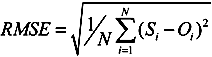
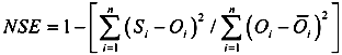
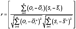
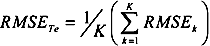
The advantage of this strategy is that all data have the chance to be trained and evaluated, giving the true error (
Te) for each error criterion (
RMSE,
Bias,
NSE, and
r). Equation (15) shows the true error of the
RMSE:
where
K is the total number of folds and
k is the index of each fold. In this study, the data set was divided randomly into four training and testing sub-sets by the cross validation method as a systematic process to obtain effective and sensitive modelling results.
3. Results and Discussion
3.1. Applications
It is expected that training data sets should cover all the characteristics of the scientific problem to obtain correct model estimations. Therefore, the data set was divided into four training and testing sub-sets by using the cross validation method as a systematic methodology to obtain effective and sensitive model findings. To get more reliable evaluations of performance of the ANFIS model, MLR given in Equation (16) was established for the 108 experimental data [
32]. As with the fuzzy approach, the four-fold cross validation method was used again.
The best model structure having four input variables was also trained and tested by ANN. The feed-forward Levenberg-Marquardt ANN network (LMNN) was used in this study. The LMNN model was trained and tested using the same non-transformed data set. The error back-propagation algorithm and tangent activation function were used for the training/testing of the LMNN model.
Figure 3b shows the typical schematic representation of a LM back-propagation neural network. The number of hidden layers and the hidden neurons within a layer, the learning rate (0.1), the coefficient of momentum (0.5) and epochs (1000) were selected by applying a trial and error method during the model training phase. The structure of the LMNN model consisted of eleven hidden neurons within one hidden layer. Details on the development of the LMNN model were presented in previous reports [
14,
33].
Table 3 summarizes the comparison of results of the ANFIS, LMNN, MLR, and empirical models.
Comparing the estimation models from
Table 3, it can be seen that
RMSE values with respect to the ANFIS model were much lower compared to the MLR and empirical models for each fold. The
RMSE values of the ANFIS model were also lower than those for the LMNN model. In addition, values for the
NSE efficiency and correlation coefficients of the ANFIS model were higher than those for the LMNN, MLR and empirical models for each fold. However, it should be noted that a trial and error procedure had to be performed for the LMNN model to develop the best network structure while such a procedure was not required for developing the ANFIS model. Moreover, in this study, the ANFIS model was trained using just 30 epochs while the LMNN model required 60 epochs. The results suggest that the ANFIS method was superior to the LMNN method in estimating the vent air discharge.
Table 3.
Values of model performance indices and error functions for the testing.
Table 3.
Values of model performance indices and error functions for the testing.
| Error Criteria | Testing Data Set | ANFIS | LMNN | MLR | Sharma | U.S. Army | Campbell | Kalinske and Robertson |
|---|
| RMSE | 1st fold | 0.242 | 0.359 | 1.024 | 6.628 | 2.233 | 2.03 | 3.325 |
| | 2nd fold | 0.221 | 0.315 | 0.734 | 5.957 | 1.912 | 1.669 | 3.147 |
| | 3rd fold | 0.286 | 0.469 | 0.867 | 7.291 | 2.272 | 1.992 | 3.661 |
| | 4th fold | 0.265 | 0.436 | 1.361 | 5.608 | 2.096 | 1.963 | 2.976 |
| NSE | 1st fold | 0.959 | 0.912 | 0.269 | −29.608 | −2.474 | −1.873 | −6.707 |
| | 2nd fold | 0.912 | 0.871 | 0.453 | −52.135 | −4.48 | −3.175 | −13.834 |
| | 3rd fold | 0.923 | 0.855 | 0.326 | −78.614 | −9.233 | −6.868 | −25.577 |
| | 4th fold | 0.923 | 0.850 | 0.440 | −9.777 | −0.506 | −0.321 | −2.036 |
| Bias | 1st fold | −0.025 | 0.021 | −0.193 | 4.994 | 1.142 | 0.965 | 2.083 |
| | 2nd fold | −0.091 | −0.183 | 0.236 | 4.497 | 1.210 | 1.023 | 2.152 |
| | 3rd fold | 0.123 | −0.338 | 0.053 | 5.357 | 1.321 | 1.119 | 2.358 |
| | 4th fold | −0.072 | −0.099 | −0.131 | 4.099 | 0.763 | 0.588 | 1.668 |
| r | 1st fold | 0.981 | 0.949 | 0.546 | −0.137 | −0.145 | −0.134 | −0.16 |
| | 2nd fold | 0.981 | 0.965 | 0.678 | 0.063 | 0.046 | 0.068 | 0.009 |
| | 3rd fold | 0.962 | 0.942 | 0.654 | −0.182 | −0.174 | −0.164 | −0.188 |
| | 4th fold | 0.972 | 0.93 | 0.632 | 0.139 | 0.142 | 0.145 | 0.125 |
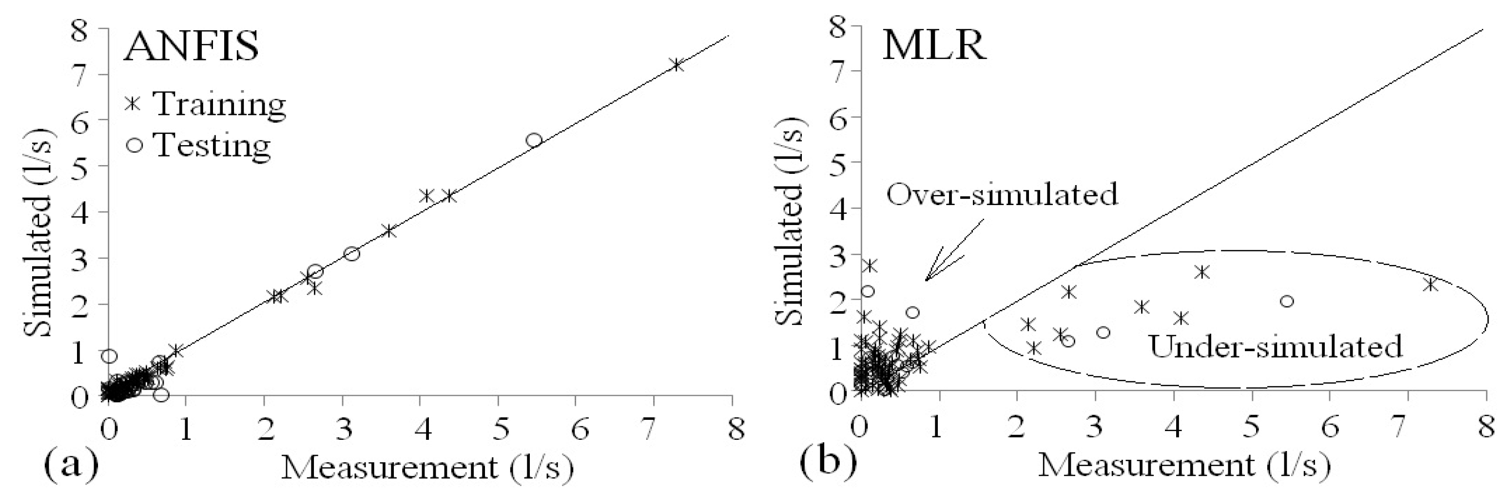
Scatter plots are displayed in
Figure 5 and
Figure 6 for the training and testing data sets, respectively.
Figure 6 shows the observed vent air discharge on the x-axis against the simulated vent air discharge on the
y-axis for the Campbell and Kalinske-Robertson’s empirical relationships.
In each of the scatter plots, a perfect estimation was placed on the 1:1 line. The ANFIS simulation (
Figure 6) fell relatively close to the 1:1 line, except for two points of the testing data set. It is interesting to note that air discharges below 1 L/s were over-simulated by empirical and MLR models whereas air discharges above 2 L/s were under-simulated. The LMNN (no figures shown) and ANFIS estimated air discharges were distributed evenly on both sides of the line of agreement. However, the data spread was more pronounced for the LMNN than for the ANFIS method.
Figure 5.
Comparing the results of Campbell and Kalinske-Robertson’s empirical models versus the observations (1st fold).
Figure 5.
Comparing the results of Campbell and Kalinske-Robertson’s empirical models versus the observations (1st fold).
Figure 6.
Comparing the results of adaptive neural-based fuzzy inference system (ANFIS) and multiple linear regression (MLR) models versus the observations (testing set of 1st fold).
Figure 6.
Comparing the results of adaptive neural-based fuzzy inference system (ANFIS) and multiple linear regression (MLR) models versus the observations (testing set of 1st fold).
3.2. Assessing Empirical, ANFIS, MLR, and LMNN Models
For comparison, performance data of the ANFIS model against the corresponding MLR and empirical models are presented in
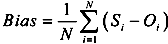
Table 4 using true error values. It is evident that the ANFIS model was by far more accurate than the empirical models and considerably more accurate than the MLR and LMNN models in terms of their simulation accuracy of the true error criteria. The ANFIS model simulated the significant air discharge parameters with an acceptable accuracy. The result of the
Bias index indicated that all empirical relationships highly overestimated air discharges (e.g.,
BiasTE for Sharma = 4.7) while the LMNN model slightly underestimated air discharges (
BiasTE = −0.15). ANFIS and MLR had normal tendencies with negligible magnitude for
Bias. The overall average values for
NSE were slightly negative.
Comparing the estimation models with each other, it can be seen that the values of RMSETe for the ANFIS model (test/0.254 and train/0.186) were lower than those for the LMNN (0.395/0.192) and MLR (0.997/0.907) models and much lower than those for the empirical models (e.g., Sharma: 6.37) for both the testing and training data sets. It appears that the NSETe of the ANFIS model (test/0.929 and train 0.982) was higher compared to the LMNN, MLR, and empirical models. In addition, the correlation coefficients of the ANFIS model (0.974/0.991) were higher than those of the LMNN (0.946/0.987), MLR (0.627/0.612) and empirical (e.g., Sharma: −0.029) models for both the testing and training sets. It should be noted that a trial and error procedure has to be performed for the LMNN model in order to develop the best network structure, while such a procedure is not required when developing the ANFIS model.
Table 4.
Performance statistics for the adaptive neural-based fuzzy inference system (ANFIS), feed-forward Levenberg-Marquardt artificial neural network (LMNN), multiple linear regression (MLR), and empirical models using true error (Te).
Table 4.
Performance statistics for the adaptive neural-based fuzzy inference system (ANFIS), feed-forward Levenberg-Marquardt artificial neural network (LMNN), multiple linear regression (MLR), and empirical models using true error (Te).
| Model | Testing set | Training set |
|---|
| RMSETe | NSETe | BiasTe | rTe | RMSETe | NSETe | BiasTe | rTe |
|---|
| ANFIS | 0.254 | 0.929 | −0.016 | 0.974 | 0.186 | 0.982 | −0.0003 | 0.991 |
| LMNN | 0.395 | 0.872 | −0.150 | 0.946 | 0.192 | 0.971 | −0.0007 | 0.987 |
| MLR | 0.997 | 0.372 | −0.009 | 0.627 | 0.907 | 0.375 | −0.003 | 0.612 |
| Sharma | 6.371 | −42.534 | 4.737 | −0.029 | | | | |
| U.S. Army | 2.128 | −4.173 | 1.109 | −0.033 | | | | |
| Campbell | 1.914 | −3.059 | 0.924 | −0.021 | | | | |
| Kalinske and Robertson | 3.277 | −12.039 | 2.065 | −0.053 | | | | |
For the ANFIS model, NSETe is 0.93, which corresponds to a perfectly modeled match to the observed data, indicating the superiority of the ANFIS model compared to both the LMNN and MLR approaches. Negative values of NSE indicated that the observed mean was a better predictor than the model. Thereafter, all the empirical models failed to simulate the air discharges properly according to the NSE criteria. In general, the results suggested that the ANFIS method is superior to the LMNN, MLR, and empirical methods for the purpose of simulating vent air discharges.
3.3. Comparison between Empirical and Computational Methods
According to empirical relationships, the air demand flow at different gate opening scenarios was determined as function of the Froude number at a contracted section according to Equations (2–5). Findings have subsequently been compared with computational relations.
Results indicate that there are considerable differences between empirical and computational methods. This could be explained by differences in the input variables used by each method. The Froude number [Equation (1)], which is used by all empirical methods as the basic parameter for estimating the air demand, includes velocity (
V) as a dependent parameter of water discharge, gate opening, and vent area (
V =
Qw / A · O) and the flow depth at the contracted section, which is a dependent parameter of water depth and gate opening (
Yc =
Y · O). Therefore, the empirical relationships are a function of four parameters:
ƒ(Qw, A, O, Y). According to the stepwise regression results (
Table 2), the second most effective input variable of estimating air flow rate is head of water (
H), which is not an input variable for the empirical relationships. This could be the reason for inferior results associated with the empirical relationships in comparison to the computational methods.
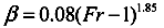
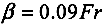
In addition to the empirical relationships, experimental data were used to assess the relationship based on non-linear regression between the Froude number (
Fr) and the aeration coefficient (
β). Equation (17) shows the best power relationship for the applied experimental data (
Figure 7).
Figure 7.
Illustration of the power relationship between the Froude number (Fr) and the aeration coefficient (β) of the applied experimental data.
Figure 7.
Illustration of the power relationship between the Froude number (Fr) and the aeration coefficient (β) of the applied experimental data.
In order to evaluate the validity of the above relationships, the statistical measures RMSE, NSE, Bias and r were calculated. Results show that the RMSE = 1.24, NSE = −0.14, Bias = −0.00036 and r = −0.045. Comparing the performance of the obtained relationships to the empirical ones [Equations (2–5)] indicates their superiority (lower RMSE, r and normal tendency for Bias) to other empirical power relationships discussed in this study. However, it should be noted that artificial intelligence models (e.g., ANFIS and ANN) do not provide an explicit expression relating the independent with the dependent variables.
4. Conclusions
Fuzzy modelling and identification of measured data are effective tools for the approximation of uncertain non-linear systems. In this paper, a TS fuzzy inference system was successfully developed and applied for the simulation of air demand discharge in low-level dam outlet works. The subtractive clustering algorithm was utilized to extract the fuzzy model structure. In order to verify the performance of the proposed approach, empirical methods (Shrama, Campbell, Kalinske-Robertson, and U.S. Army), a traditional MLR model and the more recent LMNN model were successfully built using the same data and subsequently compared with each other. The data were randomly separated into four sub-sets using the K-fold cross validation method.
The performances of the empirical models were inferior to the MLR model. The Bias index values indicated that empirical methods highly over-estimated the air demand discharges while the ANFIS model had a normal tendency. The average RMSE of four folds was 0.25 for the ANFIS model compared to 0.40 for the LMNN model, which was considered acceptable. The performance of the ANFIS model was satisfactory, considering that the average NSE efficiency values of 0.98 and 0.93 were recorded for the training and testing data sets, respectively. Lower corresponding values of NSE efficiency were computed for the LMNN (0.97/0.87) and MLR (0.38/0.37) models.
The considerable difference between the results of empirical and computational methods indicates the high degree of a non-linear relationship between water discharge and air flow rate. The use of only the Froude number as an input parameter for estimating the air flow rate was unreliable. Alternatively, the proposed fuzzy rule-based model can be used at least complementary to the empirical relationships, MLR, and artificial neural network models to assess the interactions between air demand discharge and hydro-structural parameters of low-level outlet works for dams.


 is the membership function (MF) and K is the number of fuzzy if-then rules. The consequent part of the rule base shows the rule output. In a TS fuzzy model, rule consequents are usually taken to be either crisp numbers or linear functions of the input parameters [Equation (7); layer 1].
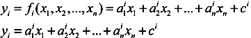
 (premise parameters in Figure 3a). The degree of matching between the input parameters and rule [Equation (6)] is called the rule firing strength (Figure 3a), which is normally defined as an and-conjunction by means of the product operator [Equation (8); layer 2].
 is the membership degree of the j-th input xj for the i-th rule. For the input x, the total output y of the TS model is computed by aggregating the contributions of individual rules [17]. Therefore, the overall fuzzy system output can be obtained by Equation (9). Consequents and outputs are shown in Figure 3a.