1. Introduction
Dissolved oxygen (below DO) content in natural waters is an indispensable quantity whenever data are collected for investigations of nature from a hydrobiological, ecological or environmental protection viewpoint [
1]. A sufficient concentration of DO is critical for the survival of most aquatic plants and animals as well as for waste water treatment [
2]. DO concentration is a key parameter for characterizing natural and wastewaters and for assessing the global state of the environment in general [
3]. The decrease of DO levels in the world’s oceans, which is becoming increasingly obvious [
3,
4,
5,
6], is expected to have an impact on the whole ecosystem of the Earth, including the carbon cycle [
7], the climate [
3,
5],
etc. The current understanding of the dynamics of the processes and their interrelation is still far from sufficient. Measurement and monitoring of dissolved oxygen concentration is essential for improving that understanding.
The majority of dissolved oxygen measurements are made with the use of amperometric [
8] and optical sensors [
9]. The performance of these sensors has dramatically improved over the years [
10]. Nevertheless, accurate DO measurement with sensors is not easy because it is influenced by numerous uncertainty sources [
8,
10,
11]. Therefore, the agreement between the sensor-based DO data from different laboratories has long been an issue and has caused a negative perception of the data using sensors in the oceanography community. Because of this, the recent issue of the World Ocean Atlas [
12] was compiled taking into account only DO concentrations obtained with chemical titration methods (first of all the Winkler titration method, WM) and rejecting all sensor-based data. A similar decision was made in a recent study of DO decline rates in coastal oceans [
6]. Yet, oceanographers need large amounts of DO data, collected continuously around the clock during lengthy time periods (months), often far away from any human settlement. Only sensor-based automatic measurements can satisfy this need. It is thus important to make every effort to underpin the quality of sensor-based measurements.
DO concentration is a highly unstable parameter of water. Thus preparation of reference solutions that are stable for extended periods of time is almost impossible. This complicates the standardization of the measurements and preparation of certified reference materials (below CRM). This is as true for Winkler titration as it is for sensor measurement of DO concentration. Also Nordtest TR 537 [
13] pointed out that there is a “long-term” uncertainty component from the variation in the calibration, which is hard to measure, as no stable reference material or CRM is available for DO measurement. The method suggested in Nordtest TR 537 for Winkler titration was to calibrate the same thiosulfate solution several times during a few days and use the variation between the results for the uncertainty estimation. Nevertheless, the highly important long-term variation component is only estimated by educated guess in Nordtest TR 537, which cannot be considered fully satisfactory and the bias component of uncertainty is not addressed at all.
However, in this paper we present a tool for laboratories: A robust method to prepare an in-house reference material—water saturated with air—for DO measurement, which will help laboratories to estimate their measurement bias. This will enable the use of the increasingly popular Nordtest approach [
13,
14] and the MUkit software [
15] for measurement uncertainty evaluation. In the Nordtest approach, among other things, control sample and routine sample replicate results are utilized for uncertainty evaluation. Also intercomparison measurement results may be exploited for uncertainty estimation with the Nordtest approach.
Intercomparison measurements are also a viable means of underpinning measurement quality with this unstable analyte. It is difficult to organize DO intercomparisons involving sending samples to the participating laboratories as is usually done in the case of interlaboratory comparisons in other chemical measurements. Given that most DO measurement instruments can be transported
in situ, interlaboratory comparisons are a good alternative. (The instrument, also called analyzer, generally consists of an amperometric or optical sensor connected to a data processing and displaying unit).
In situ interlaboratory comparisons are intercomparison measurements, where all the participants (with their own equipment and using their own competence) measure the same sample continuously at the same time, at the same site [
16]. This arrangement provides the best possibility for assessing participant performance in determining DO content in water (Participant—laboratory participating in the intercomparison and sending a worker and an instrument to the intercomparison).
Recently an international
in situ interlaboratory comparison measurement of dissolved oxygen concentration took place at the University of Tartu [
17]. The results revealed that the routine laboratories as a rule still do not fully master the art of dissolved oxygen concentration measurement. The purpose of this communication is, based on the results of the interlaboratory comparison, to examine the performance of the laboratories in different parts of the intercomparison, and based on these data, uncover the problems that the participants have and to define a set of recommendations for the improvement of their performance. Also possible future actions for improving competency of DO sensor measurement will be discussed.
2. Experimental Section of the DO Intercomparison
The ESTDO-2012
in situ interlaboratory comparison measurement of dissolved oxygen concentration took place on 23 March 2012 at the Testing Centre of the University of Tartu (below UT), Estonia. The purpose of the intercomparison was twofold: To assess the agreement between the results of DO measurements performed by the personnel of the participant laboratories with their instruments according to their usual working procedures and to improve the measurement competence of the participants. There were thirteen participants to the DO intercomparison, below denoted as:
A,
B,
C,
D,
E,
F,
G,
H,
I,
J,
K,
L and
M [
17]. The participants are listed in this report but the results are presented in random order, so that the results cannot be traced back to the participants. Every participant received a private letter revealing his/her result number and permitting assessment of performance.
The best comparison of measurement results is possible when the measured value is determined by the participants for the same object in the same location at the same time—in the so-called
in situ mode [
16]. In this intercomparison the measurements were carried out in water produced by a MilliQ Advantage A10 setup (below MilliQ water) at four saturation concentrations (according to ISO 5814:2012 [
18]), in tap water and in an oxygen-free environment at a concentration of practically 0 mg/L. The DO measurements were carried out in the apparatus shown in
Scheme 1 and
Figure 1. An additional image of the experimental setup is available from reference [
19].
Scheme 1.
The experimental setup of the dissolved oxygen (DO) interlaboratory comparison.
Scheme 1.
The experimental setup of the dissolved oxygen (DO) interlaboratory comparison.
Figure 1.
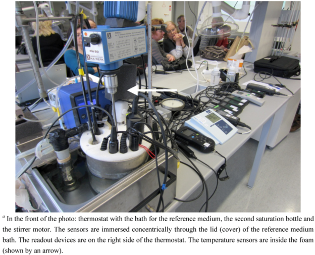
Photo of the experimental setup of dissolved oxygen intercomparison a.
Figure 1.
Photo of the experimental setup of dissolved oxygen intercomparison a.
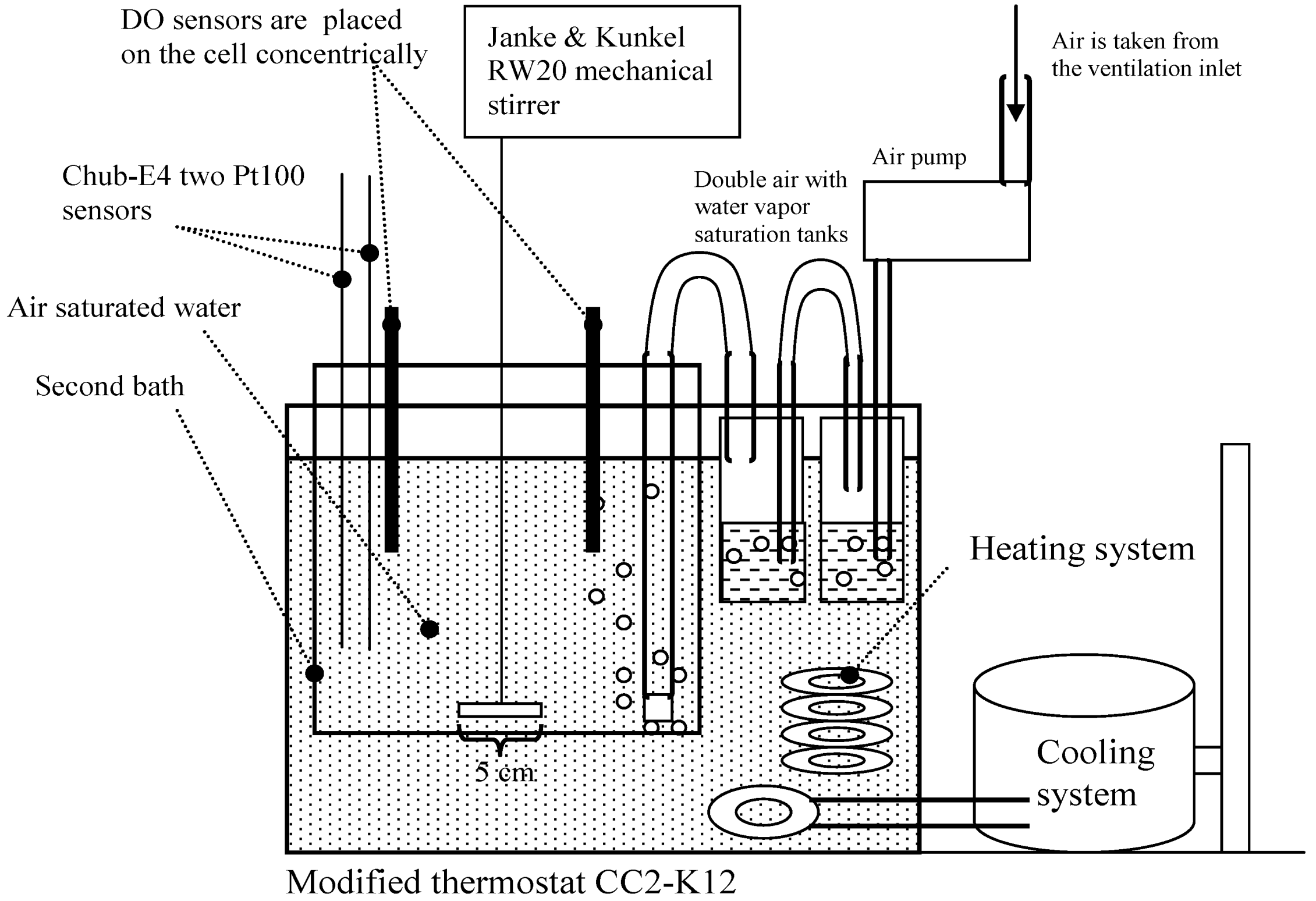
At saturation conditions the measurements were carried out as follows. Air-saturated MilliQ water was used as the reference medium (equilibrium saturation medium). The pressure, humidity and temperature of the air used for saturation were controlled and taken into account. The saturation medium was created in a modified (a second bath and a mechanical stirrer were added) thermostat CC2-K12 (Peter Huber Kältemaschinenbau GmbH, Germany) in MilliQ water with overall volume 3.9 L (
Scheme 1). The obtained temperature variability was lower than 0.01 °C (expressed as standard deviation). The air used for saturation of the reference medium was taken from the air inlet situated on the roof of the building. The air used for saturation was first saturated with water to achieve relative humidity of 100% for the air. The air flow velocity during calibration was around 1 dm
3 min
−1. The ordinary aquarium spray was used for bubbling (at a depth of 13 cm). The estimated diameter of the bubbles was between 0.8 and 1.8 mm.
The measured environment was stirred using a four-bladed stirrer with constant speed (160 rpm). Thus the DO probes of the participants were arranged concentrically in the bath and were immersed approximately to the same depth for achieving the same velocity of water movement in the location of each sensor. According to our experience over the years [
16], this setup permits achieving the best possible uniformity of the measurement conditions between the participants, and the differences between the DO concentrations in the vicinity of different sensors are negligible. Stirrer dimensions and its location in the reference medium are also given in
Scheme 1.
2.1. Calibration of Measurement Equipment
As stated above the purpose of the intercomparison was to assess the agreement between the participant results obtained using their routine work procedures. Therefore the participants were requested to carry out calibration of their measurement instruments in the same way as they would in the case of ordinary field work according to their own procedures and calibration intervals.
2.2. The Measurement Conditions
As reference values (assigned values) for DO, the theoretical DO saturation concentrations were used and they were calculated as described in the standard ISO 5814:2012 [
18]. The experimental setup for creating the water saturated with air under carefully controlled conditions and the calculation method for obtaining the reference values and their uncertainties have been verified using the gravimetric Winkler titration method [
20]. The uncertainty of the reference value was estimated according to the ISO GUM. All the major uncertainty sources, such as temperature measurement, temperature instability, air pressure, air humidity, oxygen concentration in air, the mathematical model itself, possible over- or undersaturation,
etc., were taken into account. The two most important uncertainty sources are possible over- or undersaturation and the uncertainty of the mathematical model itself [
20]. The uncertainties of the reference DO concentrations used in this intercomparison were conservatively estimated as ±0.15 mg/L (
k = 2). The temperature of the MilliQ water was measured by calibrated digital thermometer Chub-E4 (Model No. 1529, Serial No. A44623, manufacturer Hart Scientific) with two Pt100 sensors (Serial No. 0818 and 0855). The last calibration was made in May 2011 (by the Estonian NMI, AS Metrosert). The uncertainties of all temperature measurements (including the bath instability uncertainty source) are ±0.05 °C (
k = 2). The atmospheric pressure was measured by digital barometer PTB330 (Serial No. G37300007, manufactured by Vaisala Oyj, Finland, calibrated by manufacturer 19 September 2011) with uncertainty 10 Pa (
k = 2). The level of air humidity after the second saturation vessel was measured using digital hygrometer Almemo 2290–8 with sensor ALMEMO FH A646 E1C (manufacturer AHLBORN Mess- und Regelungstechnik GmbH). The humidity of the air bubbled through the water in the second bath was around 100% RH. The uncertainties of all relative humidity measurements are ±5% RH (
k = 2).
The timeline of the intercomparison is presented in
Table 1. The measurements started at the highest temperature and every new temperature was lower than the preceding one. Lowering the temperature in order to arrive at the next temperature level started immediately after taking the readings of the participant and reference instruments at the preceding temperature. Sufficient time was allowed for stabilization of the temperature and dissolved oxygen content. Both parameters were monitored and measurements were started only after a stable plateau was seen. The criterion of stability was that DO reading of the monitoring instrument (with optical sensor) did not change by more than 0.01 mg/L during 10 min. The temperature always stabilized faster than the DO reading; therefore the stability of the DO reading automatically equaled the stability of the temperature reading.
Table 1.
Timetable, reference values and uncertainties.
Table 1.
Timetable, reference values and uncertainties.
| Time window | Reference value of DO concentration | Reference value of temperature | Air pressure | Medium |
|---|
| Cref | U, k = 2 | tref | U, k = 2 | mean | U, k = 2 |
|---|
| start–end (h:min) | mg/L | mg/L | °C | °C | Pa | Pa | Comment |
| 10:39–10:47 | 8.24 | 0.15 | 24.84 | 0.05 | 100,757 | 10 | MilliQ water saturated with air (below: SAT25) |
| 12:45–12:46 | 9.07 | 0.15 | 19.91 | 0.05 | 100,757 | 10 | MilliQ water saturated with air (below: SAT20) |
| 14:38–14:42 | 10.05 | 0.15 | 15.04 | 0.05 | 100,926 | 10 | MilliQ water saturated with air (below: SAT15) |
| 16:56–17:00 | 12.74 | 0.15 | 5.07 | 0.05 | 100,932 | 10 | MilliQ water saturated with air (below: SAT5) |
| 17:25–17:28 | – | – | – | – | – | – | Tapwater at room temperature (below: TAPW) |
| 17:31–17:39 | 0.0 | 0.01 | – | – | – | – | Oxygen-free tapwater (added: Na2SO3 + CoCl2) (below: ZERO) |
3. Results
The normality of the data sets was tested according to the Kolmogorov-Smirnov normality test [
21] at 0.05 significance level using SPSS
® Statistics Version 20. The possible outliers were tested using Hampel’s test [
22]. According to the Hampel outlier test participant A produced outliers for DO measurement for all samples except SAT5. Results of participant C were outliers for samples SAT25, SAT20, SAT15 and TAPW. Results of participant H were outliers for samples SAT25 and SAT20. For temperature measurement no outliers were observed. A summary of the Kolmogorov-Smirnov normality test is given in
Table 2. The test data for sample ZERO in DO determination was not normally distributed. For all other samples the null hypothesis was retained at a significance level of 0.05. If the result of participant A was removed, then the null hypothesis was also retained for measurement results of sample ZERO. Due to the low number of measurement results all the data were included in the statistical treatment.
Table 2.
Summary of Kolmogorov-Smirnov normality tests for DO and temperature measurements.
Table 2.
Summary of Kolmogorov-Smirnov normality tests for DO and temperature measurements.
| No. | Null Hypothesis | Test | Sig. | Decision |
|---|
| 1 | The distribution of SAT25 is normal with mean 8.15 and standard deviation 0.75. | One-Sample Kolmogorov-Smirnov Test | 0.286 | Retain the null hypothesis. |
| 2 | The distribution of SAT20 is normal with mean 8.97 and standard deviation 0.99. | One-Sample Kolmogorov-Smirnov Test | 0.368 | Retain the null hypothesis. |
| 3 | The distribution of SAT15 is normal with mean 9.81 and standard deviation 1.23. | One-Sample Kolmogorov-Smirnov Test | 0.321 | Retain the null hypothesis. |
| 4 | The distribution of SAT5 is normal with mean 12.34 and standard deviation 1.14. | One-Sample Kolmogorov-Smirnov Test | 0.986 | Retain the null hypothesis. |
| 5 | The distribution of TAPW is normal with mean 7.89 and standard deviation 1.65. | One-Sample Kolmogorov-Smirnov Test | 0.112 | Retain the null hypothesis. |
| 6 | The distribution of ZERO is normal with mean 0.31 and standard deviation 0.85. | One-Sample Kolmogorov-Smirnov Test | 0.010 | Reject the null hypothesis. |
| 7 | The distribution of T25 is normal with mean 24.88 and standard deviation 0.09. | One-Sample Kolmogorov-Smirnov Test | 0.716 | Retain the null hypothesis. |
| 8 | The distribution of T20 is normal with mean 19.91 and standard deviation 0.07. | One-Sample Kolmogorov-Smirnov Test | 0.262 | Retain the null hypothesis. |
| 9 | The distribution of T15 is normal with mean 15.02 and standard deviation 0.13. | One-Sample Kolmogorov-Smirnov Test | 0.688 | Retain the null hypothesis. |
| 10 | The distribution of T5 is normal with mean 5.20 and standard deviation 0.20. | One-Sample Kolmogorov-Smirnov Test | 0.752 | Retain the null hypothesis. |
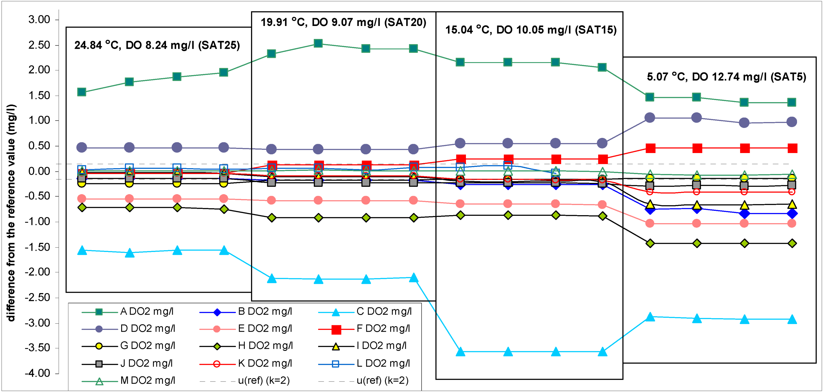
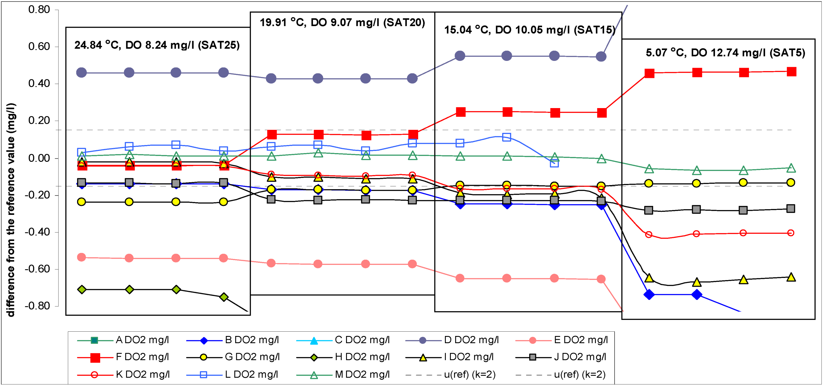
The reference DO concentration values at different temperatures are given in
Table 1. The results of the participant instruments are given in
Table 3 and differences of the readings of the participant instruments from the reference values are given in
Scheme 2,
Scheme 3.
Scheme 4 provides the same information (as in
Scheme 2) with reduced DO concentration axis. The participant results were recorded in quadruplicate at about 1–3 min intervals using digital photos. Photographing allows recording all the readings within a very short time and preserving and archiving them for the solution of possible disputes. Herein after the word “participant value” or “participant instruments result” is used with the following meaning: It is the mean of the four readings taken as explained above.
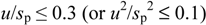
The reliability of the reference values of DO was tested according to the criterion
where
u is the standard uncertainty of the reference value (the expanded uncertainty of the reference value (
U) divided by two) and
sp the standard deviation for proficiency assessment (the true standard deviation of the participant results) [
23]. In the testing of the reliability of the reference value of DO the criterion was met in every case and the reference values were reliable.
Table 3.
DO Readings of the Participant Instruments.
Table 3.
DO Readings of the Participant Instruments.
| Medium | DO concentrations | Temperatures |
| SAT25 | SAT20 | SAT15 | SAT5 | TAPW | ZERO | SAT25 | SAT20 | SAT15 | SAT5 |
| mg/L | mg/L | mg/L | mg/L | mg/L | mg/L | °C | °C | °C | °C |
| Reference values | 8.24 | 9.07 | 10.05 | 12.74 | – | – | 24.84 | 19.91 | 15.04 | 5.07 |
| Participant | | | | | | | | | | |
| A | 10.03 | 11.50 | 12.18 | 14.15 | 12.83 | 3.00 | 24.90 | 19.90 | 14.90 | 5.10 |
| B | 8.10 | 8.90 | 9.80 | 11.95 | 7.63 | 0.10 | 24.80 | 19.90 | 15.10 | 5.68 |
| C | 6.67 | 6.96 | 6.49 | 9.83 | 5.97 | 0.17 | 24.90 | 19.90 | 15.10 | 5.20 |
| D | 8.70 | 9.50 | 10.60 | 13.75 | 8.20 | 0.20 | 25.00 | 19.83 | 14.80 | 5.00 |
| E | 7.70 | 8.50 | 9.40 | 11.70 | 7.30 | 0.10 | 24.80 | 19.90 | 15.00 | 5.40 |
| F | 8.20 | 9.20 | 10.30 | 13.20 | 7.83 | 0.00 | 24.90 | 19.90 | 15.00 | 5.30 |
| G | 8.00 | 8.90 | 9.90 | 12.60 | 7.55 | 0.00 | 25.00 | 19.90 | 14.80 | 4.98 |
| H | 7.52 | 8.16 | 9.18 | 11.31 | 7.51 | 0.05 | 24.90 | 20.00 | 15.20 | 5.30 |
| I | 8.22 | 8.97 | 9.85 | 12.08 | 7.75 | 0.04 | 24.90 | 19.90 | 15.10 | 5.10 |
| J | 8.11 | 8.84 | 9.82 | 12.46 | 7.30 | 0.01 | 24.85 | 19.93 | 15.06 | 5.08 |
| K | 8.20 | 8.98 | 9.89 | 12.33 | 7.01 | 0.03 | 24.83 | 19.91 | 15.04 | 5.07 |
| L | 8.29 | 9.13 | 10.10 | – | – | – | 24.70 | 19.80 | 15.00 | – |
| M | 8.25 | 9.09 | 10.06 | 12.68 | 7.75 | 0.04 | 25.00 | 20.08 | 15.20 | 5.20 |
Scheme 2.
Differences between DO readings of the participant instruments and the reference values (scale: +3.20 to −4.00 mg/L).
Scheme 2.
Differences between DO readings of the participant instruments and the reference values (scale: +3.20 to −4.00 mg/L).
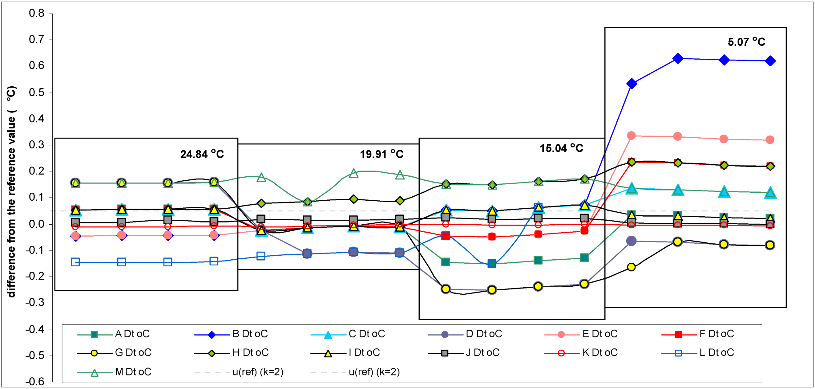
Scheme 3.
Differences between temperature readings of the participant instruments and the reference values. The estimated uncertainties of the temperature reference values are ±0.05 °C (k = 2).
Scheme 3.
Differences between temperature readings of the participant instruments and the reference values. The estimated uncertainties of the temperature reference values are ±0.05 °C (k = 2).
Scheme 4.
Differences between DO readings of the participant instruments and the reference values (reduced scale: +0.80 to −0.80 mg/L).
Scheme 4.
Differences between DO readings of the participant instruments and the reference values (reduced scale: +0.80 to −0.80 mg/L).
The mean values and standard deviations of the thirteen participating laboratories under five different sets of conditions are presented in
Table 4.
Single factor (one-way) analysis of variance (ANOVA) was applied for the data set for calculating the within-laboratory and the between-laboratory standard deviations
sw and
sb.
sw describes the repeatability of measurements, while
sb describes the reproducibility of measurements. In this proficiency test the reproducibility (
sb) was on an average two to 31 times higher than the repeatability (
sw). If the outliers were rejected, the ratio
sb/sw remained mainly below 10, being highest for samples SAT25 and SAT20 for DO measurement and T25 for temperature measurement. For the robust measurements the ratio
sb/sw should not exceed three [
24]. High values were observed mainly due to very low within-laboratory standard deviation. In this type of intercomparison, the above mentioned criterion is actually not applicable, since for the estimation of the within-laboratory standard deviation, successive measurements should be carried out in such a way that the sensor probe is taken out of the reference medium, allowed to settle to the room temperature, immersed again and then allowed to stabilize before the measurement result is recorded. However, this would have been very difficult to carry out in the setup used in our intercomparison.
Table 4.
The mean values of the participating laboratories and their absolute and relative standard deviations.
Table 4.
The mean values of the participating laboratories and their absolute and relative standard deviations.
| Medium a | DO concentration | Temperature |
| mean b | st. dev. c | % st. dev. c | mean b | st. dev. c |
| mg/L | mg/L | % | °C | °C |
| SAT25 | 8.15 | 0.75 | 9 | 24.88 | 0.09 |
| SAT20 | 8.97 | 0.99 | 11 | 19.91 | 0.07 |
| SAT15 | 9.81 | 1.23 | 13 | 15.02 | 0.13 |
| SAT5 | 12.34 | 1.14 | 9 | 5.20 | 0.20 |
| TAPW | 7.88 | 1.65 | 21 | 19.86 | 0.08 |
3.1. Assessing the Agreement between the Participant Values and the Reference Values according to the En Approach
To assess the agreement between the values of the participants and the reference values using the
En numbers [
25], uncertainty data of the participant values are needed. The uncertainties of measurement values were estimated by the participants themselves. The expanded uncertainties are presented in
Table 5.
Table 5.
The self-declared expanded uncertainties a of the participant values.
Table 5.
The self-declared expanded uncertainties a of the participant values.
| Participant | DO concentrations | Temperatures |
| SAT25 | SAT20 | SAT15 | SAT5 | TAPW | ZERO | SAT25 | SAT20 | SAT15 | SAT5 |
| mg/L | mg/L | mg/L | mg/L | mg/L | °C | °C | °C | °C | °C |
| A | 0.20 | 0.20 | 0.20 | 0.20 | – | – | 0.20 | 0.20 | 0.20 | 0.20 |
| B | – | – | – | – | – | – | – | – | – | – |
| C | – | – | – | – | – | – | – | – | – | – |
| D | 0.20 | 0.20 | 0.20 | 0.20 | – | – | 0.20 | 0.20 | 0.20 | 0.30 |
| E | 0.00 | 0.00 | 0.00 | 0.00 | 0.00 | 0.00 | 0.00 | 0.00 | 0.00 | 0.00 |
| F | – | – | – | – | – | – | – | – | – | – |
| G | – | – | – | – | – | – | – | – | – | – |
| H | – | – | – | – | – | – | – | – | – | – |
| I | 0.13 | 0.09 | 0.38 | 0.32 | 0.00 | 1.00 | 0.40 | 0.60 | 0.30 | 0.60 |
| J | 0.44 | 0.47 | 0.52 | 0.65 | 0.47 | 0.26 | 0.10 | 0.10 | 0.10 | 0.10 |
| K | 0.30 | 0.30 | 0.30 | 0.30 | 0.30 | 0.30 | 0.01 | 0.01 | 0.01 | 0.01 |
| L | – | – | – | – | – | – | – | – | – | – |
| M | 0.16 | 0.16 | 0.17 | 0.30 | 0.16 | 0.13 | 0.30 | 0.30 | 0.30 | 0.30 |
It can be seen from
Table 1,
Table 3,
Table 5 that the deviations of the participant often result from the fact that the reference values are significantly higher than the expanded uncertainties of the participants, which means that the uncertainties are in many cases underestimated. We have currently no information about the methods that were used by the participants for estimating measurement uncertainties.
The
En numbers for DO concentration are found as follows [
25]:
where
Clab is the participant DO value,
Cref is the reference value of DO concentration,
Ulab is the expanded uncertainty of the participant value and
Uref is the expanded uncertainty of the reference value.
The
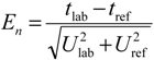
En numbers for temperature:
where
tlab is the participant temperature value,
tref is the reference temperature value,
Ulab is the expanded uncertainty of the participant value and
Uref is the expanded uncertainty of the reference value.
Criteria for laboratory performance based on the En numbers:- (a)
-
|E
n| ≤ 1:
![Water 05 00420 i009]()
(the result and reference value are accordant);
- (b)
-
|E
n| > 1:
![Water 05 00420 i010]()
(the result and reference value are not accordant).
The
En number is strongly dependent on the uncertainty of the participant value. Therefore, a close to zero
En value does not directly indicate a high quality of the participant value but only the agreement between it and the reference value (which, of course, is an important component of the quality of the result). The |
En| numbers of the participants for DO measurement under four sets of conditions (saturation concentration under four temperatures) are given in
Table 6. The |
En| numbers of the participants for temperature measurement under four sets of conditions (saturation concentration under four temperatures) are given in
Table 7.
Table 6.
The |En| numbers of the participants for DO measurement a.
Table 6.
The |En| numbers of the participants for DO measurement a.
| Medium | A | B | C | D | E | F | G | H | I | J | K | L | M |
|---|
| SAT25 | 7.1 | 0.9 | 10.4 | 1.8 | 3.6 | 0.3 | 1.6 | 4.8 | 0.1 | 0.3 | 0.1 | 0.3 | 0.1 |
| SAT20 | 9.7 | 1.1 | 14.1 | 1.7 | 3.8 | 0.9 | 1.1 | 6.1 | 0.6 | 0.5 | 0.3 | 0.4 | 0.1 |
| SAT15 | 8.5 | 1.7 | 23.7 | 2.2 | 4.3 | 1.7 | 1.0 | 5.8 | 0.5 | 0.4 | 0.5 | 0.4 | 0.0 |
| SAT5 | 5.7 | 5.2 | 19.4 | 4.1 | 6.9 | 3.1 | 0.9 | 9.5 | 1.8 | 0.4 | 1.2 | | 0.2 |
| ZERO | 20.0 | 0.7 | 1.1 | 1.3 | 0.7 | 0.0 | 0.0 | 0.3 | 0.0 | 0.0 | 0.1 | | 0.2 |
Table 7.
The |En| numbers of the participants for temperature measurement a.
Table 7.
The |En| numbers of the participants for temperature measurement a.
| Medium | A | B | C | D | E | F | G | H | I | J | K | L | M |
|---|
| SAT25 | 0.3 | 0.9 | 1.1 | 0.8 | 0.9 | 1.1 | 3.1 | 1.1 | 0.1 | 0.1 | 0.1 | 2.9 | 0.5 |
| SAT20 | 0.1 | 0.3 | 0.3 | 0.4 | 0.3 | 0.3 | 0.3 | 1.7 | 0.0 | 0.2 | 0.2 | 2.3 | 0.5 |
| SAT15 | 0.7 | 1.2 | 1.2 | 1.2 | 0.8 | 0.8 | 4.8 | 3.2 | 0.2 | 0.2 | 0.2 | 0.8 | 0.5 |
| SAT5 | 0.1 | 12.1 | 2.6 | 0.2 | 6.6 | 4.6 | 1.9 | 4.6 | 0.0 | 0.0 | 0.0 | | 0.4 |
3.2. Assessing the Agreement between the Participant Values and the Consensus Values According to the Z-Score Approach
Participant results were also evaluated according to the z-score approach [
25,
26]. The z-score for a participant value is calculated according to the following equation:
where
x is the participant’s value,
xc is the consensus value and
s is the target standard deviation. The consensus values and target standard deviations for the respective measurement conditions were found using the Algorithm A as described in the ISO 13528:2005 standard [
26]. This algorithm gives the so-called robust estimates of the consensus value and standard deviation of participants. Absolute (
i.e., unsigned) values of
z-scores (|
z| values) are used for assessing the acceptability of the DO and temperature results as described in
Table 8.
Table 8.
Criteria for laboratory performance based on the z-scores assessment.
The |
z| scores of the participants for DO measurement under six sets of conditions for DO and four for temperature measurement are presented in
Table 9,
Table 10, respectively, as well as in
Scheme 5.
Table 9.
The |z| values of the participants for DO measurement a.
Table 9.
The |z| values of the participants for DO measurement a.
| Medium | A | B | C | D | E | F | G | H | I | J | K | L | M |
|---|
| SAT25 | 4.3 | 0.0 | 3.2 | 1.3 | 0.9 | 0.2 | 0.3 | 1.3 | 0.2 | 0.0 | 0.2 | 0.4 | 0.3 |
| SAT20 | 5.1 | 0.0 | 3.9 | 1.1 | 0.8 | 0.5 | 0.0 | 1.5 | 0.1 | 0.2 | 0.1 | 0.4 | 0.3 |
| SAT15 | 4.1 | 0.2 | 6.1 | 1.3 | 0.9 | 0.7 | 0.0 | 1.3 | 0.1 | 0.1 | 0.0 | 0.4 | 0.3 |
| SAT5 | 1.4 | 0.2 | 1.7 | 1.2 | 0.4 | 0.7 | 0.3 | 0.7 | 0.1 | 0.2 | 0.1 | – | 0.4 |
| TAPW | 8.2 | 0.2 | 2.3 | 1.1 | 0.3 | 0.5 | 0.1 | 0.0 | 0.4 | 0.3 | 0.7 | – | 0.4 |
| ZERO | 34.3 | 0.3 | 1.1 | 1.5 | 0.3 | 0.8 | 0.8 | 0.3 | 0.4 | 0.8 | 0.5 | – | 0.4 |
Table 10.
The |z| values of the participants for temperature measurement a.
Table 10.
The |z| values of the participants for temperature measurement a.
| Medium | A | B | C | D | E | F | G | H | I | J | K | L | M |
|---|
| SAT25 | 0.1 | 1.0 | 0.1 | 1.2 | 1.0 | 0.1 | 1.2 | 0.1 | 0.1 | 0.4 | 0.6 | 2.1 | 1.2 |
| SAT20 | 0.2 | 0.2 | 0.2 | 1.3 | 0.2 | 0.2 | 0.2 | 1.3 | 0.2 | 0.3 | 0.1 | 1.6 | 2.4 |
| SAT15 | 0.9 | 0.5 | 0.5 | 1.6 | 0.2 | 0.2 | 1.6 | 1.2 | 0.5 | 0.3 | 0.1 | 0.2 | 1.2 |
| SAT5 | 0.3 | 2.7 | 0.2 | 0.8 | 1.3 | 0.7 | 0.9 | 0.7 | 0.3 | 0.4 | 0.5 | – | 0.2 |
Scheme 5.
The z-scores of the participants for DO and temperature measurements.
Scheme 5.
The z-scores of the participants for DO and temperature measurements.
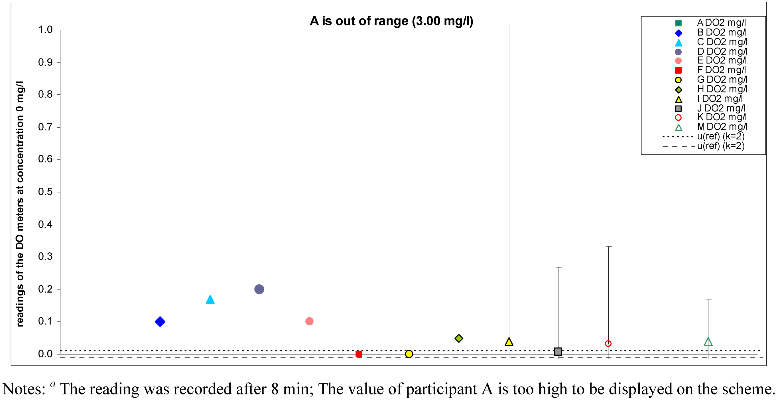
3.3. DO Measurements in an Oxygen-Free Solution
The oxygen-free solution was prepared according to the standard ISO 5814:2012 [
18] by adding saturated sodium sulfite containing a catalytic amount of cobalt chloride solution to the water. This measurement was first of all meant to check the zero values of the participant instruments. Ideally the so-called “zero value” in the zero-oxygen medium should be zero. There are no predefined criteria available for the evaluation the closeness to zero. Therefore we use criteria based on our earlier experience presented in
Table 11.
Table 11.
Criteria for laboratory performance in the zero value assessment.
Scheme 6.
Readings of participant instruments at DO concentration 0 mg/L a.
Scheme 6.
Readings of participant instruments at DO concentration 0 mg/L a.
Table 12.
Readings of participant instruments at DO concentration 0 mg/L a.
Table 12.
Readings of participant instruments at DO concentration 0 mg/L a.
| Medium | A | B | C | D | E | F | G | H | I | J | K | L | M |
| mg/L | mg/L | mg/L | mg/L | mg/L | mg/L | mg/L | mg/L | mg/L | mg/L | mg/L | mg/L | mg/L |
| ZERO | 3.00 | 0.10 | 0.17 | 0.20 | 0.10 | 0.00 | 0.00 | 0.05 | 0.04 | 0.01 | 0.03 | | 0.04 |
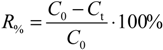
Besides the reading itself, the response time also gives useful information. A short response time means that the sensor has been designed well and is in good working order. A long response time means that the sensor is ill-designed or, in the case of amperometric sensors, the internal electrolyte needs to be replaced and the cathode/anode cleaning or replacing. Response time is usually evaluated using the so-called response factor
R%, which is defined as the percentage of reading change (from the final reading change) that occurs during a given time when the medium where the sensor is immersed changes to another:
where
C0 is the initial reading in the tap water medium,
Ct is the reading 3 min after adding the concentrated Na
2SO
3 solution.
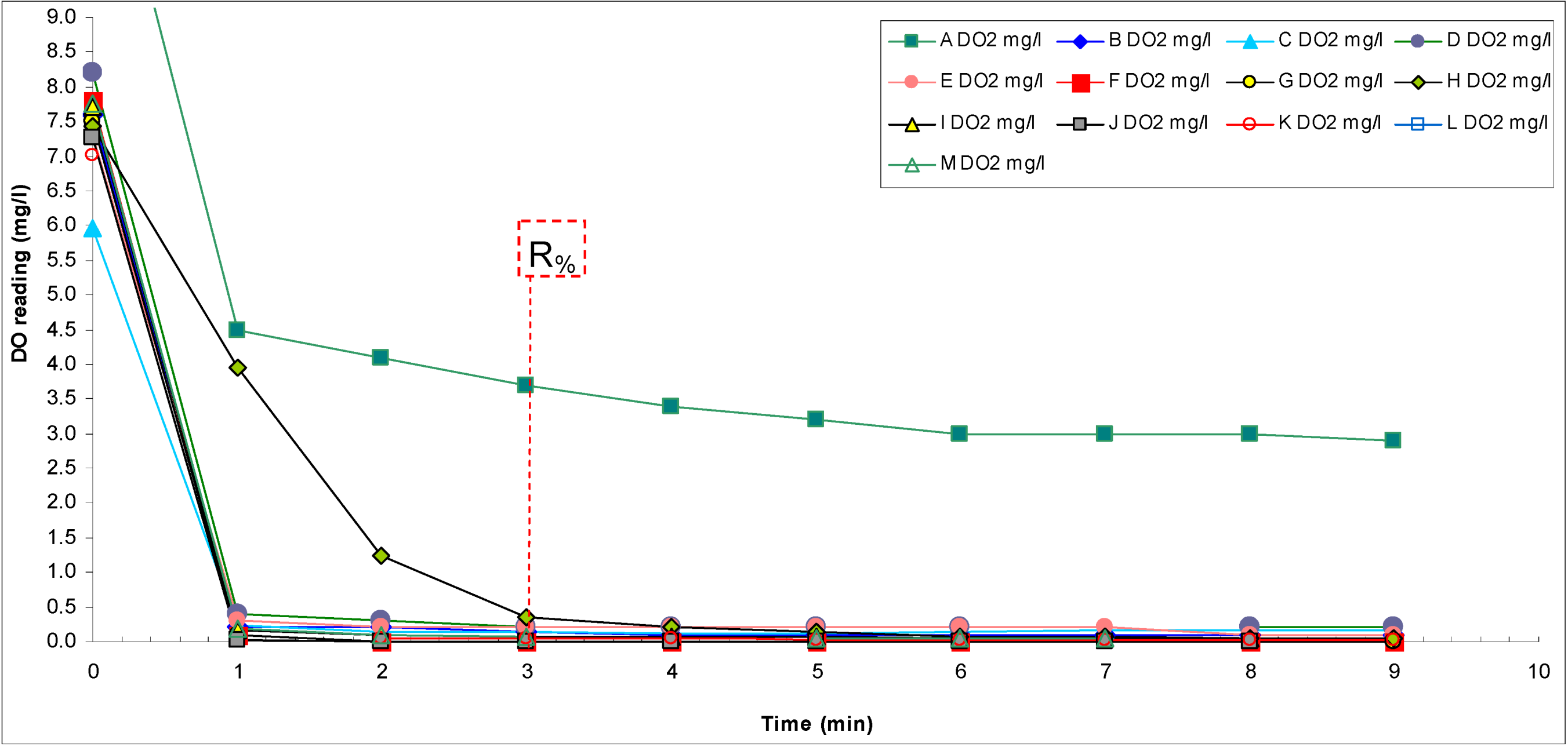
In our case the sensor was initially immersed in tap water with a DO concentration around 8 mg L
−1 and then the DO concentration was brought to zero. The readings were taken after 3 min. The criteria used for assessment of the response time are presented in
Table 13.
Table 13.
Criteria for laboratory performance based on response factor assessment.
The reading changes and response factors (R
%) are presented in
Scheme 7 and
Table 14, respectively.
Scheme 7.
Dynamics of changes in the readings of participant instruments [tap water (TAPW) → ZERO].
Scheme 7.
Dynamics of changes in the readings of participant instruments [tap water (TAPW) → ZERO].
Table 14.
The R% values of the participants.
3.4. Comparing Different Analytical Methods
DO measurement results were grouped according to sensor type used. Most of the participants used sensors based on amperometric measurement (participants A–I). Four of participating laboratories used sensors based on optical measurement. The F-test was applied to find out if there was any significant difference between variances of the DO results obtained from the two different sensor types. If outliers were not rejected, the F-test resulted in unequal variances for all sample mediums. If outliers were rejected, the F-Test resulted in unequal variances only for samples SAT25, SAT15 and SAT5. Unequal variances resulted mainly from the large distribution of the DO results obtained with amperometric sensors. The low number of observations (n = 4) with the optical sensors also made the comparison of these two measurement methods difficult. Reasons for the high scattering of the results are discussed in more detail in Chapter 4.
Two-sample t-test (two-tailed; significance level 0.05) was applied to investigate possible significant differences between averages of the results obtained by the two different sensor types. No significant differences were observed for the averages independent of whether the outliers were rejected or not.
4. Conclusions of DO Intercomparison Results
DO measurements by sensors are often deemed easy measurements by routine laboratories. In reality, the physical and chemical processes underlying the measurements are complex and these measurements are not at all as robust as often considered [
8,
16]. The results of this intercomparison fully support this statement: Out of altogether 63 measurement results obtained by the participants, 33, which corresponds to 52%, were unacceptable according to the
En numbers. According to the z-score approach, the picture is better, but still 11% of the results are unacceptable. The good performance in terms of
z-scores is largely also due to the high spread of the participant results.
Assessment of participant performance was carried out in four ways: According to
En and
z-scores, the zero value and the response factor approach (
R%). The
En approach needs both an independent reference value and uncertainty estimates from the participants. If a participant has not presented uncertainties for the results or the presented uncertainties are too optimistic then the absolute values of the
En scores are automatically inflated and may be above one even if the difference of the result from the reference value is not large. The
z-score approach uses statistical criteria only and with the small number of laboratories it is usually very mild. The last two ways are specifically meant to assess whether the sensor is in good working order.
Table 15 summarizes the findings of the organizers as recommendations for the laboratories.
According to the En numbers participants using optical sensor performed better than participants using amperometric sensor. In part this may be caused by the optical sensors being more robust in routine use than the amperometric sensors. The latter need careful and skilled maintenance and more frequent calibration in order to perform well. It is clearly seen that in many cases the amperometric sensors were not maintained and calibrated often enough. Measurement with amperometric sensors also needs more skill. However, this was not a factor in this intercomparison, because the sensors of the participants were kept immersed in the constantly stirred solution throughout the intercomparison.
Table 15.
Comments and recommendations of the organizer to the participants.
Table 15.
Comments and recommendations of the organizer to the participants.
| Participant | Sensor type | Organizer comment |
|---|
| A | amperometric | The sensor most probably is at the end of its lifetime (very high zero current and slow response). As a minimum, the electrolyte and membrane (or the whole sensing element) should be replaced. Then new calibration should be performed. Introducing a control chart for monitoring the instrument would be highly advisable. |
| B | amperometric | There is possibly a problem with the temperature measurement and/or compensation in the instrument. Uncertainty evaluation is needed. |
| C | amperometric | It is possible that the sensor is at the end of its lifetime (high zero current). The electrolyte and membrane (or the whole sensing element) should be replaced. More frequent calibration is needed. Uncertainty evaluation is needed. Introducing a control chart for monitoring the instrument would be highly advisable. |
| D | amperometric | It is possible that the sensor is at the end of its lifetime (high zero current). The electrolyte and membrane (or the whole sensing element) should be replaced. New calibration would be advisable. Introducing a control chart for monitoring the instrument would be highly advisable. |
| E | amperometric | More frequent calibration is needed. Uncertainty evaluation is needed. Introducing a control chart for monitoring the instrument would be highly advisable. |
| F | amperometric | There is possibly a problem with the temperature compensation in the instrument. Uncertainty evaluation is needed. Introducing a control chart for monitoring the instrument would be highly advisable. |
| G | amperometric | More frequent calibration is needed. Uncertainty evaluation is needed. Introducing a control chart for monitoring the instrument would be highly advisable. |
| H | amperometric | It is possible that the sensor is at the end of its lifetime (slow response). Calibration is needed. Uncertainty evaluation is needed. Introducing a control chart for monitoring the instrument would be highly advisable. |
| I | amperometric | There is possibly a problem with the temperature compensation in the instrument. Introducing a control chart for monitoring the instrument would be highly advisable. |
| J | optical | – |
| K | optical | – |
| L | optical | Participated in too few measurements to give an overall assessment. Uncertainty evaluation is needed. |
| M | optical | – |
6. Discussion and Future Plans
The current intercomparison revealed that a number of participants did not report uncertainties for their results, even though most of them are accredited according to the ISO/IEC 17025 [
30], which states that competent laboratories must evaluate their measurement uncertainties (unless the nature of the measurements precludes this). Use of “in-house” reference material and routine sample replicate results together with control charts enable laboratories to estimate measurement uncertainty of the DO measurement with the Nordtest approach [
13] more easily and more reliably than before. Näykki
et al. recently published a paper presenting software support for the measurement of uncertainty evaluation based on the Nordtest approach [
15]. In addition setting up control charts and participating in interlaboratory comparison tests may be exploited to check if the self-declared uncertainty estimate is realistic [
31].
Even though we managed to arrange the
in situ intercomparison for DO and we may even have, in a controlled way, produced “in-house” reference material for dissolved oxygen measurement, the reference medium in both cases is deionized water, which may be far from the real sample matrix. The needs of the oceanographic community to compare their Seabird-type sensors—designed for use in the sea—are important to note. It was not possible during the ESTDO-2012 to include the Seabird-type sensors, because of the limited size of the setup used. More intercomparisons with real natural water sample matrix are needed, and one such
in situ comparison is planned to be arranged in 2014 for DO measurements in the Baltic Sea area in Finland in the framework of the European Metrology Research Programme project ENV05 “Metrology for ocean salinity and acidity” [
32]. In this study, the DO measurements will be carried out directly on a ship with the “real sample”—low salinity seawater.
It remains first of all to the laboratories themselves to find out what their problems in particular cases are. However, the organizers hope that the present intercomparison will help them find the right direction.


