Soil Erosion and Surface Water Quality Impacts of Natural Gas Development in East Texas, USA

Abstract

Due to greater demands for hydrocarbons and improvements in drilling technology, development of oil and natural gas in some regions of the United States has increased dramatically. A 1.4 ha natural gas well pad was constructed in an intermittent stream channel at the Alto Experimental Watersheds in East Texas, USA (F1), while another 1.1 ha well pad was offset about 15 m from a nearby intermittent stream (F2). V-notch weirs were constructed downstream of these well pads and stream sedimentation and water quality was measured. For the 2009 water year, about 11.76 cm, or almost 222% more runoff resulted from F1 than F2. Sediment yield was significantly greater at F1, with 13,972 kg ha⁻¹ yr⁻¹ versus 714 kg ha⁻¹yr⁻¹ at F2 on a per unit area disturbance basis for the 2009 water year. These losses were greater than was observed following forest clearcutting with best management practices (111–224 kg ha⁻¹). Significantly greater nitrogen and phosphorus losses were measured at F1 than F2. While oil and gas development can degrade surface water quality, appropriate conservation practices like retaining streamside buffers can mitigate these impacts.

1. Introduction

Recent advances in drilling technology have resulted in a dramatic expansion in exploration for and development of oil and natural gas. Historically, single vertical wells were drilled into hydrocarbon traps in permeable rock formations where gas and oil had migrated to. Starting in the 1940s, water, sand, and other additives under high pressure were used to fracture low permeability hydrocarbon source rocks like shales. Due to the high cost of these operations relative to the value of the oil and gas recovered, this practice had only limited applicability. Recent advances in horizontal drilling technology coupled with higher prices for oil and natural gas have resulted in a significant increase in hydraulic fracturing or fracking. In addition, CO₂ emissions from natural gas combustion are 30%–40% lower than coal, NOx emissions are 80% lower for natural gas, and emissions are almost 100% lower for SO₂, particulates, and mercury compared with coal [1]. Therefore, natural gas is seen as an acceptable bridge fuel until more sustainable energy sources become viable. This will likely result in greater development of natural gas resources in the future.

One area of very active drilling in the United States is East Texas, southwestern Arkansas, and western Louisiana. The Haynesville, Cotton Valley, Travis Peak, and other formations underlie this region and have been very productive, with a drilling success rate of over 99%. The Haynesville shale has been the most productive formation and is between 3.1 and 4.3 km deep and about 91 m in thickness [2]. It is estimated to contain about 7 trillion m³ of natural gas [3]. Drilling increased by over 300% in the Haynesville region from 2008 to 2012.

There are numerous concerns associated with oil and gas development and water resources. These include firstly, the large amount of water used in fracking. In the Barnett shale, fracking water use in 2010 was 308 Mm³, or about 9% of the total water used by the city of Dallas, Texas [4]. In addition, concerns exist about the possibility of fracking fluids contaminating aquifers. With regards to surface waters, leaking pipelines, reserve pits, and producer water spills are a significant hazard [5]. Finally, concerns exist about the erosion and sedimentation that can result from natural gas development. Sedimentation is among the greatest contributors to stream impairment in the United States [6].

In the Barnett shale region of north Texas, sediment yields from natural gas sites in Denton County were 54 t ha⁻¹ yr⁻¹, much greater than the 1.1 t ha⁻¹ yr⁻¹ measured from undisturbed rangelands in this region [7]. The United States Environmental Protection Agency (USEPA) regulates small construction sites (0.4 ha or greater) for stormwater discharge and sediment movement. In the state of Texas, gas wells are not regulated by the state environmental agency as small construction sites and are not subject to the same regulations. In addition, little regulatory oversight is given to how the placement of well pads may impact surface water resources.

Best management practices (BMPs) to control stormwater discharge and nonpoint pollution for other industries like agriculture and forestry have been widely adopted in the USA. For example, over 95% of forestry operations in Texas employ these BMPs [8], and these BMPs have been proven to be very effective in reducing sedimentation from clearcutting and site-preparation [9]. Similarly, it is estimated that sedimentation from natural gas well sites could be reduced by as much as 93% by using BMPs [10].

The purpose of this study was to quantify the stormwater concentrations and losses of sediment, nutrients, and metals from a natural gas well site. Comparisons were made between a gas well site constructed in the stream channel and a site offset from the stream channel by 15 m to determine the extent to which well location may affect sediment loss and water quality. Comparisons were also made between these water quality impacts and impacts from other land uses in the watersheds.

2. Materials and Methods

2.1. Study Area

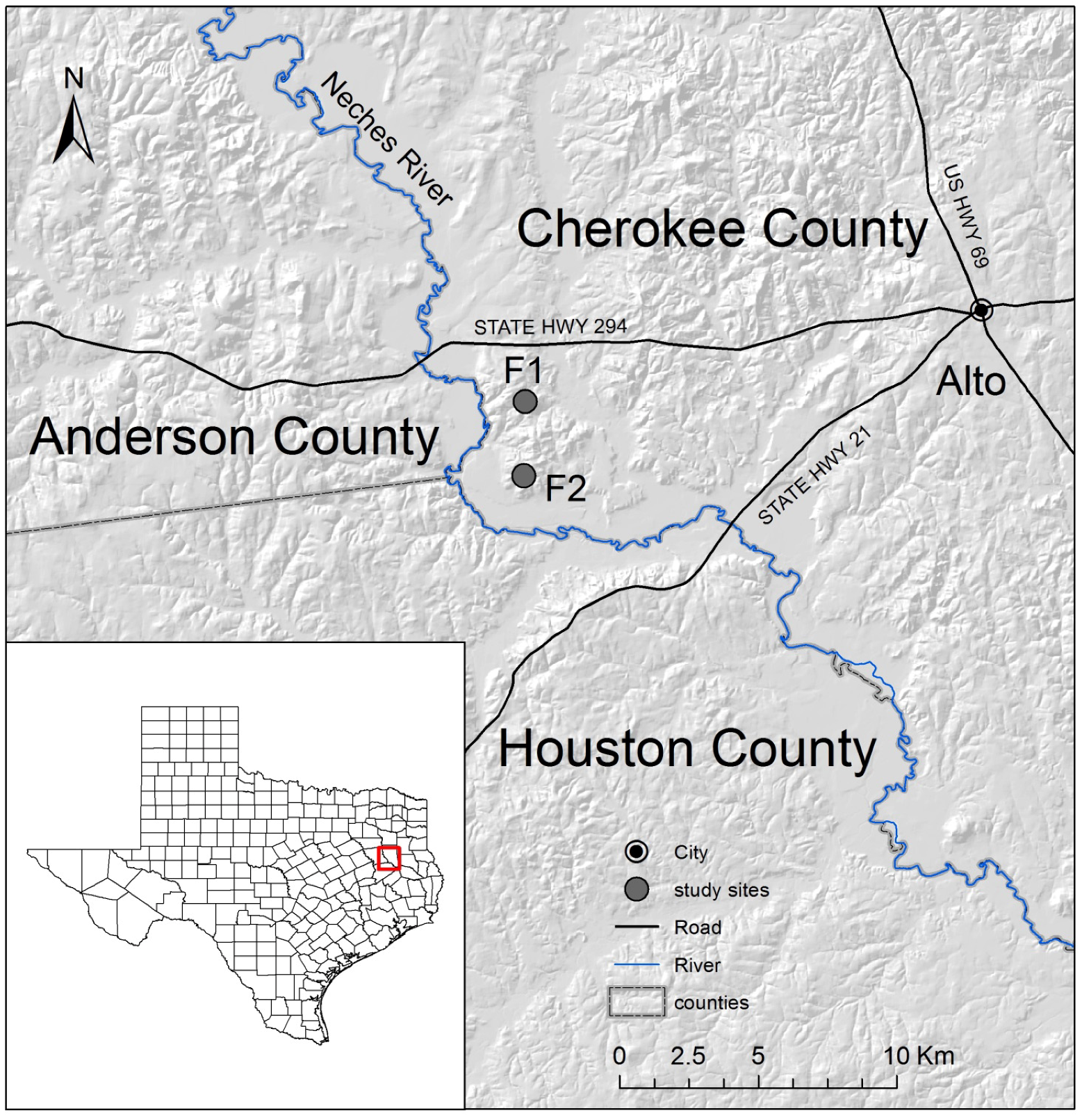
The study was conducted at the Alto Experimental Watersheds in the Neches River basin approximately 16 km west of the town of Alto in Cherokee County, Texas, USA (Figure 1). The study area is in the Gulf Coastal Plain and has a humid subtropical climate. Average summer temperatures are 27.2 °C and average winter temperatures are 9.5 °C, with a mean annual temperature of 18.7 °C. Annual rainfall in the region is 117 cm. The rain is distributed fairly evenly throughout the year with an average of 89 rain days a year, with April and May receiving the largest amount of rainfall [11].

Figure 1. Location of study watersheds (F1 = no riparian buffer, F2 = 15 m riparian buffer) at the Alto Experimental Watersheds in Cherokee County, Texas, USA.

Figure 1. Location of study watersheds (F1 = no riparian buffer, F2 = 15 m riparian buffer) at the Alto Experimental Watersheds in Cherokee County, Texas, USA.

The soils at the Alto Experimental Watersheds formed in Eocene sediments. The dominant surface formations are members of the Claiborne Group and are Sparta Sand and the Cook Mountain Formation [12]. These soils developed under mixed loblolly pine (Pinus taeda) and hardwood forests, have low inherent fertility and are most commonly classified as Alfisols and Ultisols. The most prevalent soil found in the watersheds is the Sacul Series (fine, mixed, active, thermic Aquic Hapludults) followed by the Tenaha Series (loamy, siliceous, semiactive, thermic Arenic Hapludults). Both soils are Ultisols with an argillic horizon and less than 35% base saturation. Teneha soils are well drained and runoff is negligible to medium with increasing slope [13]. Sacul soils are slowly permeable soils that formed in acidic, loamy and clayey marine sediments. They are moderately well drained with medium to very high runoff potential, and have a seasonally high water table that is within 61 to 122 cm of the soil surface in late winter and spring most years [13].

2.2. Treatments

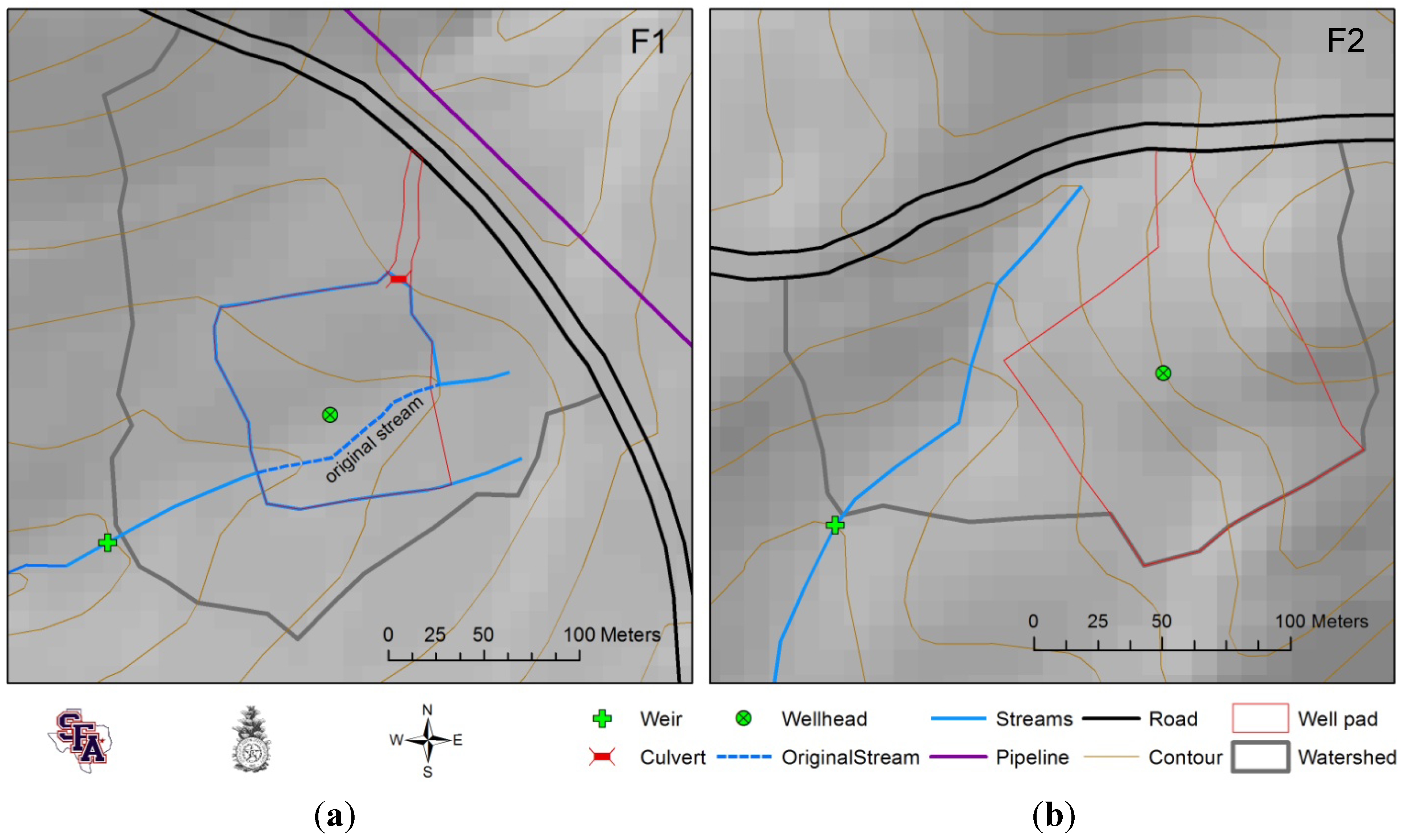
In the spring of 2008, two natural gas wells were drilled. At the first site (F1), the well pad was constructed directly in the channel of an intermittent stream and has a watershed area of 13.7 ha with the pad comprising 1.4 ha (Figure 2a). The stream was rechanneled around the north side of the pad following construction. At the second site (F2), the pad was offset from the creek channel by about 15 meters; this site has a watershed that consists of 4.5 ha with the well pad occupying 1.1 ha (Figure 2b).

In the process of constructing the well pad at F-1, fill material had to be brought in from an undisclosed location. The fill material consisted of 55.5% sand and 44.5% clay. Once this fill material had been brought in and the site leveled, iron ore gravel (16–150 mm diameter) was hauled in and spread over the majority of the pad with the exception of approximately one-quarter of the western end of the pad, which was used for a drilling fluid reserve pit. After drilling was completed, the reserve pit was filled with soil that was 40.2% sand, 14.1% silt, and 45.7% clay. This area was then seeded with ryegrass (Lolium spp.) While some of the seeds germinated, most did not grow or were carried away by surface runoff, resulting in bare soil.

The well pad at F2 required no fill material for pad construction due to the topography of the site. F2 was placed on the southern face of a large hill. Earth-moving equipment was used to modify the hill from a steep slope to a 1.1 hectare terrace suitable for operating large drilling equipment on. This soil was 65.1% sand, 9.5% silt, and 25.3% clay. After the terrace was constructed, iron ore gravel was spread similar to the method employed at F1. The back, southern portion used as a reserve pit for drilling fluids. The soil used to fill in the reserve pit was 21.7% sand, 32.1% silt, and 46.2% clay.

Both sub-watersheds where the gas well sites were constructed were dominated by loblolly pine. The northern portion of the F1 watershed was mixed hardwoods and pine; this area comprised approximately 3.5 hectares. The rest of the F1 watershed was 10–15 year old loblolly pine plantation. Approximately 2 hectares of the F2 watershed was 10–15 year old loblolly pine plantation while the rest was a mixed hardwood and pine stand. The portion of the watershed that was mixed hardwood and pine was composed of fairly large (≈50–100 cm) timber. These larger diameter trees consisted primarily of white and red oaks (Quercus spp.) and loblolly pine. This area of large mixed timber at both watersheds was the result of timber harvests in compliance with Texas BMPs, leaving the riparian forest as a contiguous buffer known as a streamside management zone (SMZ). The understory of both watersheds consists mostly of species such as dogwood (Cornus florida), sweetgum (Liquidambar styraciflua), various magnolias (Magnolia spp.), various hickories (Carya spp.), yaupon (Ilex vomitoria), sassafras (Sassafras albidum), and American beautyberry (Calicarpa americana).

Figure 2. F1 (a) and F2 (b) natural gas well pad layout at the Alto Experimental Watersheds, Texas, USA.

Figure 2. F1 (a) and F2 (b) natural gas well pad layout at the Alto Experimental Watersheds, Texas, USA.

2.3. Water Quantity and Quality

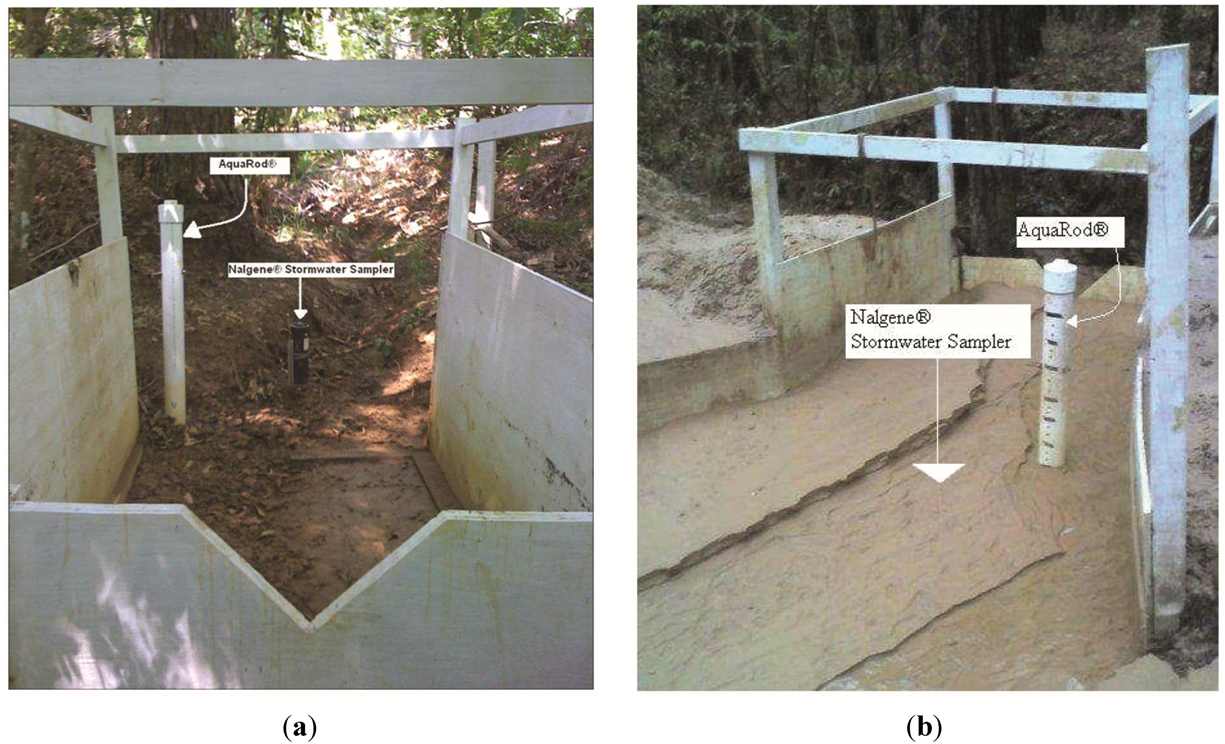
In both streams, a v-notch weir was constructed approximately 80 m downstream from the pad (Figure 3).

In each weir, an AquaRod^® water level monitor was installed in the mouth of the flume. Unfortunately, stage data obtained from the AquaRods^® were unreliable due the unexpectedly high sediment loads deposited in the weirs burying the capacitance rods. Streamflow was therefore estimated using the ArcAPEX model from precipitation measured at the sites [14]. ArcAPEX was calibrated and validated for these watersheds in earlier studies [15]. Rain gauges were located throughout the watershed and after each storm event precipitation data were collected.

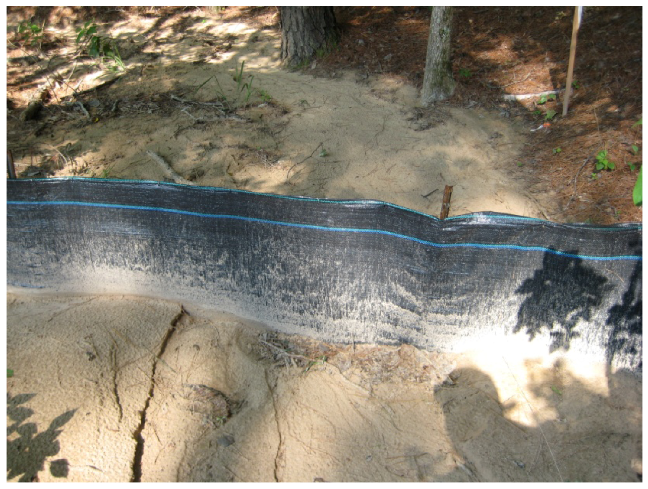
As a result of the streamflow being ponded by the front plate of the weir, the coarse sediments were deposited in the drop box section on the floor of the weir. After each rain event this sediment was removed and weighed to determine the amount of sedimentation occurring in the stream channel (Figure 4). Dry mass was determined from a sub-sample of this sediment. The amount of sediment deposited in the drop box was later added to the amount of suspended sediment losses in stormflow. These losses were quantified using the flow estimated by ArcAPEX multiplied times the total suspended sediment (TSS) values that were obtained from stormwater samples. Sampling occurred from September 2008 to March 2010.

Water samples were collected from each weir using one of two techniques. The first technique utilized a Nalgene^® Storm Water Sampler (Figure 3). Within 24 h of each storm runoff event the sample bottle was removed and a clean, acid rinsed bottle was placed in the cylinder. These samplers were frequently buried by the large volumes of sediment. When this occurred, the second method was used, the grab sample method, in which a 1 L sample bottle was placed in the flow of the stream and a water sample was taken. Grab samples typically represented the recession phase of the hydrograph. Once the samples were collected from the field they were brought to the laboratory for analysis. The samples in the lab were analyzed using a Hach^® DR/890 Datalogging Colorimeter and a Hach^® sensION 156 Portable pH/Conductivity Meter according to approved United States Environmental Protection Agency (USEPA) methods [16]. Parameters analyzed included total suspended solids (TSS), total dissolved solids (TDS), pH, conductivity (EC), total nitrogen (TN), ammonia (NH₄⁺), nitrate nitrogen (NO₃⁻), nitrite nitrogen (NO₂⁻), total phosphorus (TP), ortho-phosphate (PO₄⁺) sulfate (SO₄⁺), iron (Fe), turbidity, color, salinity, calcium hardness and magnesium hardness. A paired T-test was employed to determine if mean water quality values were different by site at = 0.05.

Figure 3. In-channel instrumentation for measuring total runoff (V-notch weir), stream level (Aquarod^®), water quality (Nalgene^® Stormwater Sampler), and sediment (drop box) on the F2 sub-watershed before a storm event (a) and after a 6.3 cm rain event in April, 2009 at F1 (b); at the Alto Experimental Watersheds in Texas, USA.

Figure 3. In-channel instrumentation for measuring total runoff (V-notch weir), stream level (Aquarod^®), water quality (Nalgene^® Stormwater Sampler), and sediment (drop box) on the F2 sub-watershed before a storm event (a) and after a 6.3 cm rain event in April, 2009 at F1 (b); at the Alto Experimental Watersheds in Texas, USA.

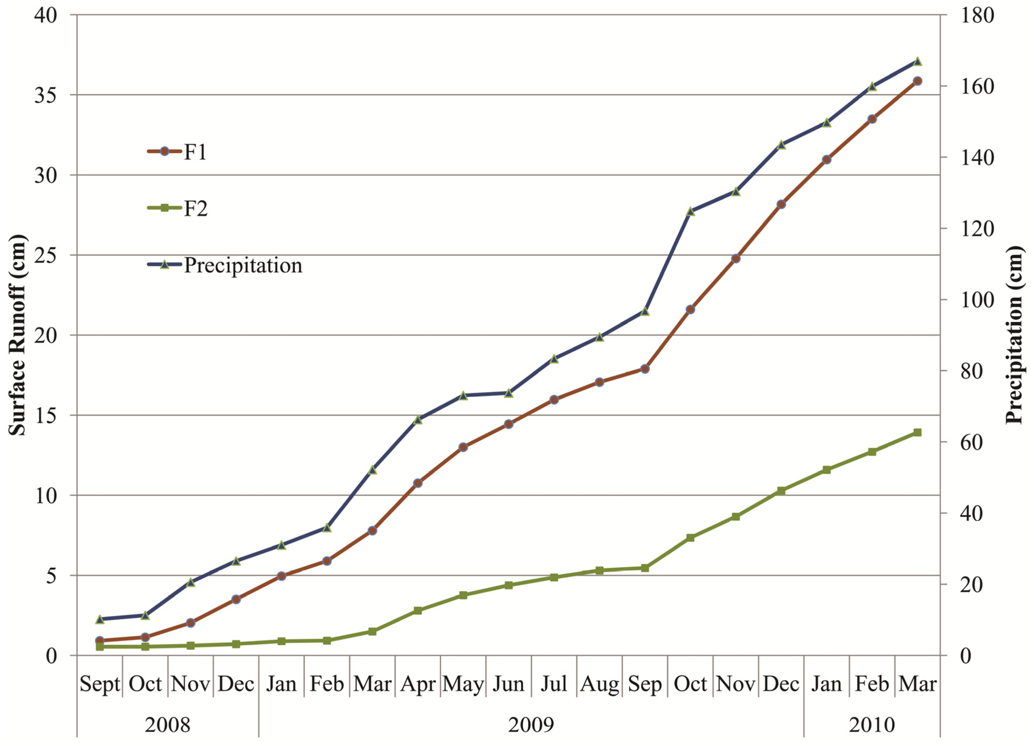
Figure 4. Cumulative ArcApex simulated water yield and rainfall for two natural gas well locations, one placed directly in the stream channel (F1) and the other offset from the channel by a 15 m buffer (F2) at the Alto Experimental Watersheds, Texas, USA.

Figure 4. Cumulative ArcApex simulated water yield and rainfall for two natural gas well locations, one placed directly in the stream channel (F1) and the other offset from the channel by a 15 m buffer (F2) at the Alto Experimental Watersheds, Texas, USA.

3. Results

In the small forested watersheds of East Texas, stream flow in headwater streams is typically intermittent and is mostly a product of storm runoff. The simulated water yield at F1 was significantly greater (p < 0.0001) than the water yield at F2 (Figure 4). In the first month of data collection (September 2008) the water yield at F1 was 0.915 cm and 0.545 cm at F2. Due to lower than average precipitation in the month of October, there was a decrease in storm runoff, but this decrease was most pronounced at F2, with 0.216 cm and 0.001 cm at F1 and F2 respectively. This trend continued throughout the study period, regardless of season. Percent runoff efficiency (runoff divided by precipitation) was different for two watersheds, 33.0% at F1 and 12.3% at F2.

Soil compaction of the well pad was much greater than in the rest of the watershed. The mean bulk density of the well pad at F1 was 2.04 g cm⁻³. Mean bulk density measurements taken in the surrounding watershed were 1.3, 1.19, and 0.99 g cm⁻³ for logging sets, skid trails, and undisturbed forest floor respectively.

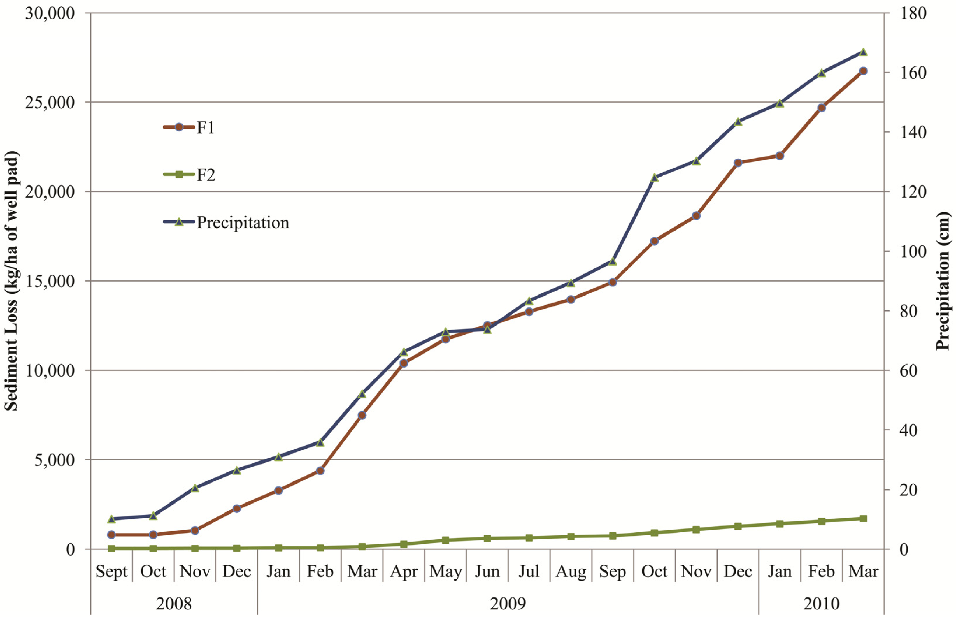
Sediment yield was also significantly greater (p < 0.001) from F1 that F2 (Figure 5). Starting in September 2008, the sediment yield was 83 kg ha⁻¹ at F1 versus 10 kg ha⁻¹ at F2. Continuing through the winter of 2009, the total yield continued to increase at F1 over F2. The total sediment yield for the 2009 water year (September 2008–August 2009) was 19,561 kg versus 785 kg at the F1 and F2 watersheds, respectively. However, this does not take into account the differences in the percent of the watershed that was actually disturbed by the well site. The well site occupied about 24% of the total watershed area at F2 versus about 10% at F1. Therefore, it is also useful to compare the sediment yields per unit area disturbed by natural gas development in order to make meaningful comparisons with the clearcut watersheds. On this basis, the equivalent sediment losses for F1 and F2 were 13,972.1 and 714 kg ha⁻¹yr ⁻¹ for the 2009 water year respectively, or 16,896 and 1,087 kg ha⁻¹yr ⁻¹ for F1 and F2, respectively, annualized for the entire 19 month (September 2008–March 2010) study period. About 56% of the sediment loss recorded at F1 was deposited in the flume, with less than 44% moving in the suspended form. However, at F2, 98% of the sediment moved in the suspended form over the study period, with only 2% being deposited in the flume. Since sediment filled the flume on F1 for several runoff events, it is possible that these loss values underestimate the amount of coarse sediments actually eroded from the pad.

Figure 5. Cumulative sediment yield and rainfall for two natural gas well locations, one placed directly in the stream channel (F1) and the other offset from the channel by a 15 m buffer (F2) at the Alto Experimental Watersheds, Texas, USA.

Figure 5. Cumulative sediment yield and rainfall for two natural gas well locations, one placed directly in the stream channel (F1) and the other offset from the channel by a 15 m buffer (F2) at the Alto Experimental Watersheds, Texas, USA.

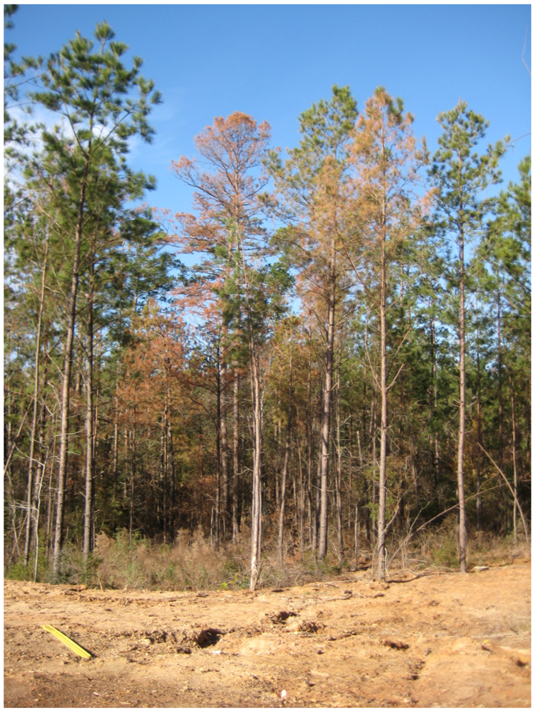
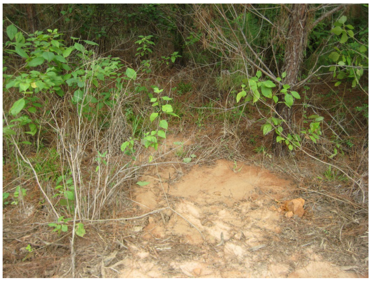
In terms of concentrations of other water quality parameters, differences between F1 and F2 were less pronounced (Table 1). For nutrients, only PO₄⁺ was significant, with the mean value being significantly greater at F2 than at F1. At F1, pH was also significantly greater, though these values were well below the Texas water quality standard minimum value of 6.0. Color was significantly greater at F1 than F2, probably associated with the higher amounts of sediment eroded from the pad at F1. However, there were no significant differences in either TSS or TDS. Salinity was significantly greater at F1 than F2, and this could have been attributed to an accidental spill of saline producer water that occurred in October 2008, but more sampling would have been required to establish this. The volume and chemical properties of this salt water was spilled was not tested. However, this spill did result in the death of several loblolly pine trees and understory vegetation down gradient of the well pad (Figure 6).

When nutrient and metal concentrations were converted to mass losses per hectare, all of the losses were greater from F1 than F2, with TDS, TN, NO₃⁻, PO₄⁺, SO₄⁺, and Fe being significantly greater (α < 0.05) using the T-test (Table 2). Since streamflow was significantly greater at F1 throughout the study period (Figure 4), it would be expected that mass losses would also be greater.

Table 1. Mean concentrations for water quality parameters measured below two natural gas well sites (F1 and F2) from October 2008–March 2010 at the Alto Experimental watersheds in East Texas, USA.

Water quality parameter	Mean1		T-test p-value
	F1	F2
Total Nitrogen (TN, mg L−1)	2.78	2.50	0.26
Ammonia (NH4+, mg L−1)	1.55	0.57	0.27
Nitrate (NO3−, mg L−1)	2.78	0.74	0.15
Nitrite (NO2−, mg L−1)	0.02	0.03	0.50
Total Phosphorus (TP, mg L−1)	0.57	0.72	0.59
Ortho-Phosphate (PO4+, mg L−1)	0.16	0.30	0.01
Total Suspended Solids (TSS, mg L−1)	335.72	288.33	0.40
Total Dissolved Solids (TSD, mg L−1)	281.43	415.44	0.13
pH	4.90	4.53	0.04
Conductivity (μS cm−1)	461.06	554.65	0.30
Color (CU)	1231.28	576.58	0.04
Calcium Hardness (mg L−1)	1.23	0.75	0.23
Magnesium Hardness (mg L−1)	2.81	2.95	0.87
Iron (Fe, mg L−1)	5.55	4.36	0.18
Salinity (mg L−1)	0.24	0.41	0.02
Sulfate (SO4+, mg L−1)	6.43	5.30	0.23

Note: ¹ Bold underlined values were significantly greater based on the paired t-test at α = 0.05.

Table 1. Mean concentrations for water quality parameters measured below two natural gas well sites (F1 and F2) from October 2008–March 2010 at the Alto Experimental watersheds in East Texas, USA.

Water quality parameter	Mean1		T-test p-value
	F1	F2
Total Nitrogen (TN, mg L−1)	2.78	2.50	0.26
Ammonia (NH4+, mg L−1)	1.55	0.57	0.27
Nitrate (NO3−, mg L−1)	2.78	0.74	0.15
Nitrite (NO2−, mg L−1)	0.02	0.03	0.50
Total Phosphorus (TP, mg L−1)	0.57	0.72	0.59
Ortho-Phosphate (PO4+, mg L−1)	0.16	0.30	0.01
Total Suspended Solids (TSS, mg L−1)	335.72	288.33	0.40
Total Dissolved Solids (TSD, mg L−1)	281.43	415.44	0.13
pH	4.90	4.53	0.04
Conductivity (μS cm−1)	461.06	554.65	0.30
Color (CU)	1231.28	576.58	0.04
Calcium Hardness (mg L−1)	1.23	0.75	0.23
Magnesium Hardness (mg L−1)	2.81	2.95	0.87
Iron (Fe, mg L−1)	5.55	4.36	0.18
Salinity (mg L−1)	0.24	0.41	0.02
Sulfate (SO4+, mg L−1)	6.43	5.30	0.23

Note: ¹ Bold underlined values were significantly greater based on the paired t-test at α = 0.05.

Table 2. Total values for mass losses (kg ha⁻¹) for water quality parameters measured below two natural gas well sites (F1 and F2) from October 2008–March 2010 at the Alto Experimental Watersheds in East Texas, USA.

Water quality parameter	Sum1		T-test p-value
	F1	F2
Total Nitrogen (TN)	10.84	3.08	0.00
Ammonia (NH4+)	4.55	0.67	0.112
Nitrate (NO3−)	11.84	0.84	0.035
Nitrite (NO2−)	0.10	0.05	0.217
Total Phosphorus (TP)	2.53	1.42	0.059
Ortho-Phosphate (PO4+)	0.72	0.47	0.042
Total Suspended Solids (TSS)	1,196	418	0.000
Total Dissolved Solids (TDS)	969	559	0.032
Iron (Fe)	19.2	5.54	0.001
Sulfate (SO4+)	21.53	6.43	0.000

Note: ¹ Bold underlined total values were significantly greater based on the paired t-test at α = 0.05.

Table 2. Total values for mass losses (kg ha⁻¹) for water quality parameters measured below two natural gas well sites (F1 and F2) from October 2008–March 2010 at the Alto Experimental Watersheds in East Texas, USA.

Water quality parameter	Sum1		T-test p-value
	F1	F2
Total Nitrogen (TN)	10.84	3.08	0.00
Ammonia (NH4+)	4.55	0.67	0.112
Nitrate (NO3−)	11.84	0.84	0.035
Nitrite (NO2−)	0.10	0.05	0.217
Total Phosphorus (TP)	2.53	1.42	0.059
Ortho-Phosphate (PO4+)	0.72	0.47	0.042
Total Suspended Solids (TSS)	1,196	418	0.000
Total Dissolved Solids (TDS)	969	559	0.032
Iron (Fe)	19.2	5.54	0.001
Sulfate (SO4+)	21.53	6.43	0.000

Note: ¹ Bold underlined total values were significantly greater based on the paired t-test at α = 0.05.

Figure 6. Mortality of loblolly pine overstory trees (red/brown needles) and understory vegetation at F2 at the edge of the streamside buffer strip following an accidental spill in October 2008 of saline water produced during natural gas extraction at the Alto Experimental Watersheds in Texas, USA.

Figure 6. Mortality of loblolly pine overstory trees (red/brown needles) and understory vegetation at F2 at the edge of the streamside buffer strip following an accidental spill in October 2008 of saline water produced during natural gas extraction at the Alto Experimental Watersheds in Texas, USA.

4. Discussion

4.1. Storm Runoff

Total runoff from these two natural gas well locations was much greater than would be expected from undisturbed areas in this region. In the undisturbed forested areas, direct surface runoff is uncommon. However, due to the significant increase in bare, compacted soils surface runoff was much more frequent. In addition, the significantly higher bulk density on the well locations resulted in less infiltration. McBroom et al. [17] found that for nearby undisturbed forests, annual runoff ranged between 0.64 and 10.32 cm, depending on rainfall. Following clearcutting of the watersheds reported by McBroom et al. [17], annual runoff ranged between 7.82 and 9.79 cm. This was comparable to runoff measured at F2 in the 2009 water year of 9.58 cm. However, the clearcut reported by McBroom et al. [17] covered an average of 75% of the total watershed area, where the well location at F2 only occupied about 10% of the total watershed area. Even when the gas well pad was offset by 15 m from the stream, it still had a proportionally greater impact on runoff than forest management. For the well pad directly in the stream channel, the effects on runoff were much greater, with 24.67 cm of runoff in the 2009 water year. In addition, runoff efficiency following clearcutting on adjacent watersheds increased from 1% pre-harvest to 9% post harvest, compared with 33% and 12% on F1 and F2, respectively.

4.2. Sediment Losses

In terms of total sediment yield, results from this study are much greater than reported from proximate watershed studies, indicating the greater relative impact of natural gas development. For undisturbed forestlands, sediment yield averaged about 42 kg ha⁻¹ [17]. Following clearcut harvesting and site preparation in 2003, losses increased from 111 to 224 kg ha⁻¹ yr⁻¹, though these differences were not found to be statistically significant [17]. In that study, a streamside management zone (SMZ) with a minimum total width of 30 m was retained around all stream channels. In 1981 these same watersheds were clearcut harvested and no SMZ was retained, and the following site preparation, sediment losses averaged 2917 kg ha⁻¹ first year after harvest [18]. Losses returned to levels measured in undisturbed forests by the second year after harvest in both 1981 [18] and in 2003 [15]. While large sediment plumes were observed to have eroded from both gas well locations, at F2 lobes of coarser sediments were trapped by the riparian vegetation and surface cover before reaching the stream channel. On F1, the 13,972 kg ha⁻¹ of disturbance for 2009 largely resulted from sediment moving from the fill slope on the back side of the pad directly into the stream channel (Figure 7).

Construction of a natural gas well location in Denton, Texas resulted in 54,000 kg ha⁻¹ yr⁻¹ of erosion [7]. This represents sediment that eroded from the pad, but may not have necessarily entered the stream channel. Using the RUSLE 2.0 model, Waschal et al. [10] concluded that good sediment control practices and BMPs can reduce sediment yields from natural gas well pads by 52%–93%. Similarly in the current study, the 94% difference in sediment between F1 and F2 can be attributed in part to the 15 m riparian buffer on F2 and better stormwater management.

One area of continued concern on F1 is that no efforts at site stabilization or revegetation were attempted following the initial failed attempt at seeding with rye grass. Significant rill and small gully erosion resulted from storm runoff flowing off the compacted pad area and down onto the sloping fill material where the reserve pit had been. Unlike results reported by Williams et al [7], after four years, the F1 well pad continued to erode with little evidence of natural stabilization, and natural vegetation remained sparse due to the poor condition of this fill material as a plant growing medium.

Similar to what was found with natural gas wells in the Fernow Experimental Forest in West Virginia, silt fences were inadequate at stopping these large sediment volumes [19]. Silt fences were installed down-gradient of the well location during construction, but they were installed about 0.25 m above the old stream channel on F1 and were overwhelmed by the large sediment loads, making silt fence ineffective at controlling these large volumes of sediment (Figure 8). Like with the wells constructed in the Fernow [19], improper installation resulted in the ineffectiveness of silt fence as a stormwater BMP. Silt fences functioned as intended on F2 due to proper installation and a lower overall sediment load that did not overwhelm their design capacity.

Figure 7. Sediment plume below the F2 natural gas well location trapped by riparian forest vegetation before entering the stream channel at the Alto Experimental Watersheds in Texas, USA.

Figure 7. Sediment plume below the F2 natural gas well location trapped by riparian forest vegetation before entering the stream channel at the Alto Experimental Watersheds in Texas, USA.

Figure 8. Silt fence installed below the natural gas well pad at F1 illustrating the ineffectiveness of this sediment control technique due to poor installation and large sediment volumes eroded at the Alto Experimental Watersheds in Texas, USA.

Figure 8. Silt fence installed below the natural gas well pad at F1 illustrating the ineffectiveness of this sediment control technique due to poor installation and large sediment volumes eroded at the Alto Experimental Watersheds in Texas, USA.

Beyond the continued erosion of the well pad, another significant concern that exists is that this deposited sediment will have long term consequences for the aquatic ecosystem. The original stream channel below the well on F1 was buried by about 0.5 m of sediment and the original pool, riffle, and glide aquatic habitats were obliterated. Sediment loading of this magnitude can have dramatic effects on lotic food webs [20]. For streams in the southeastern United States, hundreds of years if not millennia may be required to naturally purge large volumes of sediments out of regional stream and river networks [21]. This represents a localized legacy sediment issue comparable to what occurred in this region due to poor agricultural practices in the 19th Century. Effective and systematic implementation of soil conservation practices is needed to ensure that significant land use alterations do not impair surface waters in regions with extensive natural gas development.

4.3. Water Quality

The effects of natural gas development on water quality parameters were less significant than with sedimentation. Concentrations of most parameters were not significantly different between F2 an F1. However, overall runoff volumes were greater at F1 than F2, so when concentrations were converted to mass losses, the most of the water quality parameters were significantly greater at F1 than F2. The larger runoff volumes from F1 may have diluted the concentrations, but the overall mass export was significantly greater. This indicates that reducing the export of nutrients and metals from natural gas well pads is dependent on effective stormwater management. At F1, there was no buffering between the well pad and the stream, meaning that direct contributions of contaminants occurred without the benefits of filtration provided by riparian buffer strips.

As noted in the Results section, a producer water spill at F2 did result in the death of several trees along the stream channel, and this may account for the significantly higher salinity values at F2 (Figure 6). Differences in water quality were not observed with other parameters. Ground water was pumped into the stream channel immediately after the spill for several days in order to dilute the effects of the spill. While the water quality of the spilled water was not characterized, this remediation measure may have been adequate to reduce the impacts on water quality parameters that could be directly measured. However, the death of the riparian trees immediately in the flow area of the spill indicates that the direct ecological effects may require different remediation strategies.

5. Summary and Conclusions

Natural gas development is important for maintain economic prosperity and for providing a necessary energy source until renewable energy sources become more viable [22]. However, significant impacts on surface water resources were measured in this study when a gas well pad was constructed with little attention given to surface drainage patterns. Unfortunately, this was not an isolated incident on this lease area, with a pad being constructed in a perennial stream a few km north from F1 and another pad platted and surveyed over another intermittent stream nearby. Erosion rates that result from this practice are orders of magnitude greater than other land uses in this region. The 13,972 kg ha⁻¹ yr⁻¹ per unit disturbance area recorded at F1 for the 2009 water year compared with the 714 kg ha⁻¹ yr⁻¹ recorded at F2 indicates that natural gas wells can be constructed without significant water quality degradation when necessary erosion control measures are implemented. However, once stream channels are filled in and obliterated, remediative BMPs like silt fence and revegetation are unlikely to have a significant effect in reducing erosion and minimizing aquatic habitat degradation. The stormwater generated by even relatively small rain events washed pollutants directly off the pad into the stream, with no opportunity for deposition and filtration.

Since construction of gas well pads in the state of Texas is not currently regulated like other construction sites, the responsibility for ending the practice of stream channel obliteration for gas well pad construction falls on the industry to self-regulate this practice. There is a precedent for effective industrial self-regulation in Texas, where forest practices like clearcutting along intermittent and perennial streams are not regulated by state or federal environmental agencies. After research demonstrated that clearcutting could have significant impacts on water resources [23], voluntary BMPs that restrict forest harvesting along streams were adopted by the forest industry in Texas by the mid-1980s. After an extensive education and outreach campaign, 98% of forestry activities in Texas voluntarily retained streamside buffers by 2011 [8]. Like the production of wood and fiber, development of natural gas resources is necessary for society. However, this must be conducted with effective and systematic implementation of soil and water conservation practices that ensure these land use changes will not impair surface waters in regions where extensive natural gas development will occur.