A Non-Stationary and Directional Probabilistic Analysis of Coastal Storms in the Greek Seas

Abstract

The variability of coastal storms over the years and direction is considered in a unified, innovative approach, providing crucial information for a wide variety of coastal engineering studies and wave energy applications under the impact of climatic change. Specifically, an alternative easy-to-apply technique is presented and applied to consider the storms’ direction as a covariate. This technique enables the probabilistic representation of coastal storms in every direction over the directional domain and is efficiently incorporated into a non-stationary directional extreme value analysis. The developed methodology is applied to six locations in the Greek Seas. Based on the derived results, the most likely and most extreme significant wave height estimates present, in general, a bimodal behavior with pronounced maxima. In particular, the first peak is observed before the twenty-first century, while the second peak is likely to occur around the middle of the twenty-first century. Furthermore, coastal storms coming from directions of large fetches are the most severe storms, presenting though a drop in their intensity at the end of the twenty-first century. On the contrary, coastal storms of fetch-limited directions may present minor variations in their probability distributions over the years.

1. Introduction

The climate change effects on coastal areas are mainly related to mean sea level (MSL) increases in combination with considerable variations in the severity, frequency of occurrence, and direction of storm events [1,2,3]. The coastal environment, human society, and infrastructure (e.g., [4]) can be highly vulnerable to extreme storms and climate change, especially when they are exposed to severe flooding and damage. Thus, the long-term forecasting of the intensity of storms in the coming decades will contribute to the immediate decision-making to mitigate or deal with these phenomena.

In particular, the long-term variations and trends in MSLs [5,6,7,8,9] received the most outstanding scientific interest until recently. Additionally, the climate change effects on extreme wave events and storm surges have also started to gain considerable attention in the last years [10,11,12,13,14,15,16,17].

These studies usually use a non-stationary extreme value analysis (NS-EVA) that is an extension of the more conventional stationary extreme value analysis (EVA). The EVA and NS-EVA are widely applied (e.g., [18,19,20,21]) and provide useful tools for numerous applications, such as the design and reliability and resilience assessment of marine and coastal structures (e.g., [22,23,24,25]), storm-induced coastal flooding (e.g., [26,27]), and coastal erosion (e.g., [28,29]), as well as the design of wave energy facilities (e.g., [30]). It is noted that an EVA assumes that the underlying probability distribution of the data remains constant over time [31]. On the other hand, an NS-EVA allows the distribution to vary over time, considering seasonal or long-term trends and changes in the wave climate.

Although a significant number of scientific studies (e.g., [15,32,33]) have focused on long-term variations in storm characteristics, namely the significant wave height, peak wave period, and storm surge, the storms’ directionality is most times ignored, and in such cases a unidirectional analysis is applied. Sometimes the wave directionality is considered in a stationary extreme value analysis (e.g., [30,34]), or in a few recent studies it was incorporated in a combined analysis of the significant wave height of storms with covariates such as the direction and season (e.g., [35]). The fact that these two kinds of variations (time (years) and direction) are rarely both considered in the same analysis is attributed to the different mathematical procedures and models involved and the use of some non-automated methods applied for the incorporation of the two components, namely the directional and non-stationary methods.

Nevertheless, the incorporation of wave directionality into a non-stationary extreme value analysis is a gap in the current practice that needs to be filled. This is mainly because such an achievement would be significantly useful in the context of coastal engineering and oceanography, where the analysis of extreme wave events is of major importance. For instance, the design and performance of coastal and port structures is remarkably affected by their orientation with respect to the extreme events’ direction. Additionally, the extreme events’ regime is often subject to long-term variations regarding their magnitude and the storms’ characteristics due to climate change. Therefore, these types of structures might require enhancement or even redesign in the case of a remarkable alteration of the extreme events’ intensity and directionality.

Being motivated by this gap in the current literature, the main research goal of the present paper is the consideration of this directional component in a non-stationary extreme value analysis of the historical, present, and future wave climates. To accomplish this, an integrated analysis is developed based on the current literature—an alternative technique to consider a storm’s direction as a covariate, with some simplifications. This integrated analysis could be called the non-stationary directional extreme value analysis (NS-DEVA), as it is a statistical technique that is implemented to analyze and represent non-stationary time series, such as the extreme significant wave height, which varies over time and is directional in nature.

The adopted methodology is applied to wave climate data from six coastal locations in Greece, near Athos, Mykonos, Heraklion, Rhodes, the Saronic Gulf, and Pylos. Then, the results of the storms’ peak $H_{\mathrm{m}0}$ probability distribution and its return values are presented as a function of the time (expressed in years) and direction, and a comparative analysis is performed between the coastal extreme wave climates in the six locations. In this manner, the effect of climate change on the coastal storm intensity and direction in Greece is investigated.

2. Materials and Methods

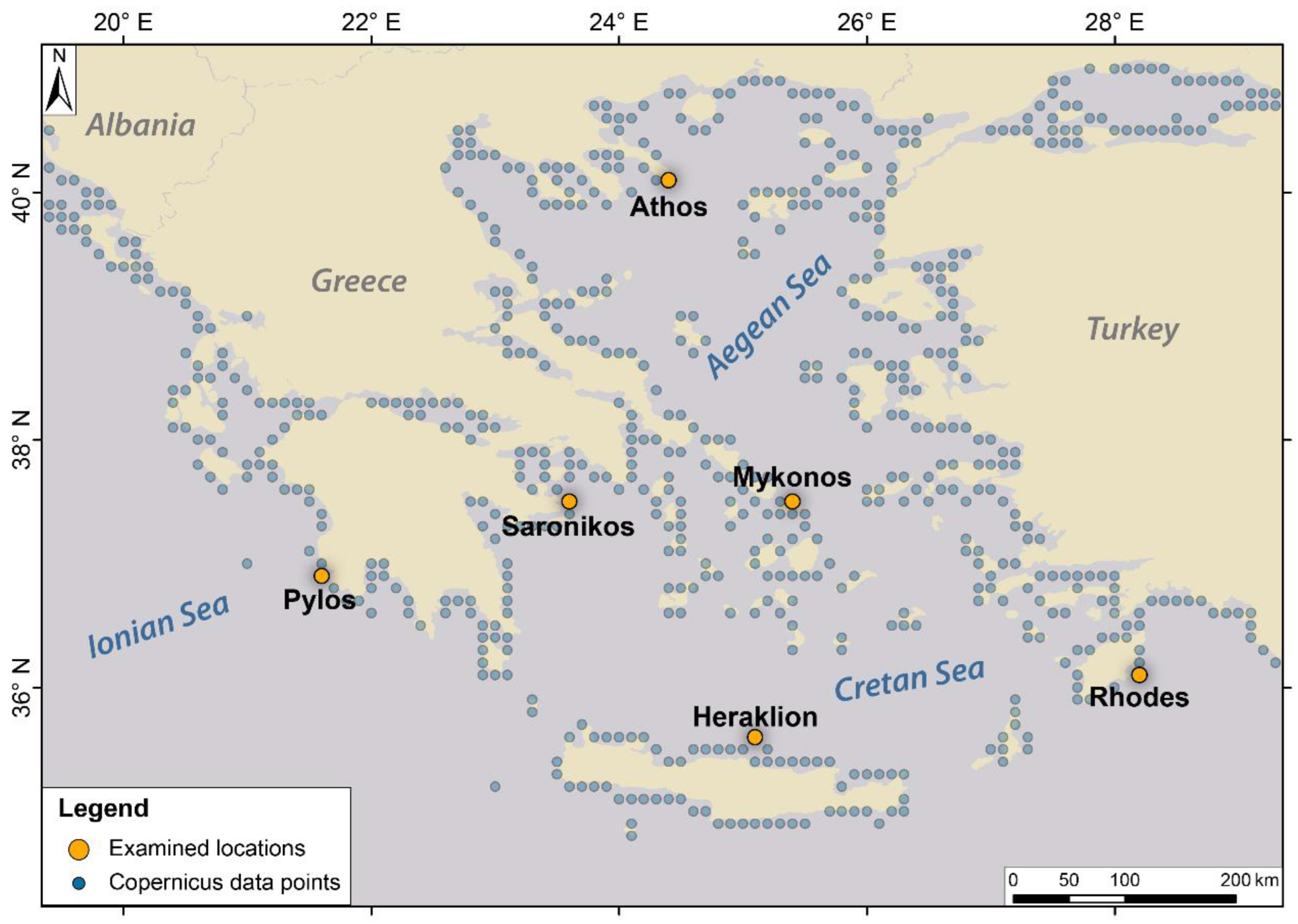
2.1. Case Studies

In the present work, ocean surface wave time series were extracted from the Climate Copernicus Database for 6 locations (see

Table 1. Examined area names and geographical locations.

s/n	Area	Latitude, Longitude (°)	Water Depth (m)
1	Athos	40.1 N, 24.4 E	840
2	Mykonos	37.5 N, 25.4 E	32
4	Heraklion	35.6 N, 25.1 E	650
4	Rhodes	36.1 N, 28.2 E	1080
5	Saronikos	37.5 N, 23.6 E	135
6	Pylos	36.9 N, 21.6 E	710

, Figure 1) in the Greek Seas. The first case study is near the peninsula of Athos in the northern Aegean; the second location is on the northern side of Mykonos island in the central Aegean, and the third one is near Heraklion in the Cretan Sea. The fourth interest point is located in the southeastern side of Rhodes in the southeastern Aegean, the fifth location is at the southern limit of the Saronic bay, and the sixth case study is near Pylos in the Ionian Sea. The six case studies are referred to from now on according to their nearby areas’ names: Athos, Mykonos, Heraklion, Rhodes, Saronikos, and Pylos. These six examined locations were selected because they cover a wide area of the Greek Seas. Additionally, their geographical locations near coastal areas make them suitable for coastal applications and engineering studies, such as the design of ports and coastal structures and the coastal areas’ protection against storm-induced erosion or flooding. Furthermore, the different orientations of the six examined locations capture all possible storms affecting the Greek coasts.

2.2. Wave Climate Description

For the needs of the present paper, time series of the significant wave height and mean wave direction were extracted from the Copernicus database at the six locations mentioned above (see orange points in Figure 1). The Copernicus data are computed using the ECMWF’s wave model (SAW) forced by surface wind data and also considering the ice coverage at polar latitudes. In order to assess the impact of climate change on the ocean’s surface wave field, the SAW model is run for the current climate scenario (also termed historical) covering the 1976–2005 era, the recent historical wave climate for the years 2001–2017 (computed using ERA5 reanalysis wind forcing), and the RCP 4.5 scenario for the years 2041–2100. The wave climate in the RCP 4.5 scenario is simulated using wind forcing from the HIRHAM5 regional climate model downscaled from the global climate model EC-EARTH [36].

The RCP 4.5 scenario was chosen as the future climate projection scenario in this paper. The RCPs (representative concentration pathways) include four pathways developed for long-term climate modeling, spanning the range of radiative forcing values from 2.6 to 8.5 W/m² [37]. RCP 4.5 is considered to be the intermediate scenario among the four scenarios. It includes long-term global emissions of greenhouse gases, short-lived species, and land use–land cover data, and stabilizes radiative forcing at 4.5 W m⁻² in the year 2100 without ever exceeding that value [38]. It is a moderate climate projection scenario and the most probable baseline scenario (no climate policies) for climate modeling regarding declining emissions and radiative forcing stabilization, taking into account the exhaustible character of non-renewable fuels (e.g., [39,40]); thus, it is used in the present paper.

The time resolution period is 1 h, while data are provided for the European coastline along the 20 m bathymetric contour and the offshore spatial coverage is 30 km. Furthermore, it is worth mentioning that since these climate scenario projections are based on a single unification of the global and regional climate models, this could lead to an underestimation to some degree of the inherent uncertainty of this dataset [36].

It is clarified here that there is a gap in the data in the used time series between the years 2017 and 2041. Additionally, in the overlapping period of the historical and recent historical datasets between 2001 and 2005, the recent historical data were used in the present paper as our focus was on the recent and future climates, and in these periods the data should be derived from an analysis that is as similar as possible.

A preliminary analysis is applied first to the extracted wave data at the six points of interest, resulting in the derivation of some basic linear statistics for $H_{\mathrm{m}0}$ and some circular statistics for $MWD$, considering its discontinuity at 360 degrees [41] (see

Table 2. Basic linear statistics for significant wave height values and circular statistics for mean wave direction values for the six examined locations.

s/n	Location	Mean ${\mathit{H}}_{\mathbf{m}0}$ (m)	Median ${\mathit{H}}_{\mathbf{m}0}$ (m)	Max. ${\mathit{H}}_{\mathbf{m}0}$ (m)	Stand. Dev. ${\mathit{H}}_{\mathbf{m}0}$ (m)	Mean $\mathit{M}\mathit{W}\mathit{D}$ (deg.)	Stand. Dev. $\mathit{M}\mathit{W}\mathit{D}$ (deg.)
1	Athos	0.69	0.46	6.94	0.68	77.35	80.81
2	Mykonos	0.95	0.76	9.03	0.74	355.57	74.36
4	Heraklion	0.94	0.77	8.44	0.70	328.05	55.54
4	Rhodes	0.58	0.43	6.37	0.52	236.90	83.71
5	Saronikos	0.49	0.35	5.44	0.46	26.89	97.66
6	Pylos	0.88	0.63	9.03	0.75	280.29	55.80

) and the wave rose diagrams (Figure 2). At Athos Point, the prevailing wave directions range from 45 to 120 degrees from north, while in Mykonos the case study is from −15 degrees to 45 degrees from north, justified by the different wind fetches and wave regimes at the two locations. Additionally, Heraklion is characterized by an extreme wave climate from directions ranging between −75 degrees and 45 degrees from north. Rhodes’s interest point presents coastal storms with directions falling between 105 degrees and 225 degrees from north.

Furthermore, the location of Saronikos is characterized by lower extreme waves compared to the other examined locations due to the limited fetch length over a wide directional sector. Notably, the 2.5 m significant wave height corresponds to the 99.5 percentile of data for Saronikos Point, while in all the other examined locations this value corresponds to a lower percentile. For instance, in the Pylos case study, the 2.5 m $H_{\mathrm{m}0}$ value corresponds to the 95.5 percentile, where extreme waves usually come from the west and northwest directions. The highest maximum values $H_{\mathrm{m}0}$ (9.03 m) are encountered at Pylos and Mykonos, although they are combined with different directions, namely 232 degrees and 356 degrees from north, respectively. The lowest $H_{\mathrm{m}0}$, mean, median, and maximum values correspond to the Saronikos case study among the rest of the examined locations.

2.3. Methodology

2.3.1. Summary

A moving time window analysis, in combination with an independent directional sector analysis and also a directional extreme value model, are applied in the present paper. The independent directional sector analysis is applied first and is also utilized to validate the results of the directional model, following Karathanasi et al. [30]. The directional model is applied to storm data at each time step, and its incorporation into the non-stationary directional extreme value analysis (NS-DEVA) enables the probabilistic representation of coastal storms concerning the time and direction by neglecting their short-term and insignificant variability (see Figure 3).

The final results are the return values of the storm’s peak $H_{m0}$ as a function of the storm’s $MWD$ and time (expressed in years). The return values will also be presented with their bounds for 95% confidence intervals.

2.3.2. Non-Stationary Directional Extreme Value Analysis (NS-DEVA)

In this study, the adopted methodology is based on running statistics using a moving time window analysis to estimate the long-term statistics as a function of time. A moving time window $W_t$ of 30 years length was applied in this study, shifted by one year every time step, as this is a reasonable time period for observing significant variations in climate (e.g., [42,43]).

Following Bender et al. [44], the time window length should satisfy two fundamental conditions: (1) it should be adequately short for the assumption of stationarity to be quite sound; (2) it should also be large enough so that the fitted probability distribution can represent the data properly and reliably. The stationarity of all moving windows was checked via the Mann–Kendall trend test [45] and the Cox–Stuart trend test [46] at a 5% significance level. In the present study, very few datasets did not pass the tests, and these cases were singles ones, implying that the stationarity requirement was met for all moving windows.

Each $W_t$ corresponds to the center of its length regarding its time step and has a length of 30 years, except for the time windows near the limits of the dataset period that have a smaller length than 30 years. However, it is recommended here that their lengths be no less than 15 years to reduce the statistical uncertainty of the results at the corresponding time steps. Then, for each $W_t$, a directional analysis is performed based on a preliminary analysis applied to 8 successive independent directional sectors, at 45 degrees in width (e.g., [30,34]). In particular, the directional sectors’ limits are 0–45 degrees, 45–90 degrees, etc., while each sector is represented by its central value.

Focusing here on the independent sector analysis, storms are identified for each directional sector and at each time step. It is widely accepted that the identification of coastal storms is achieved through the use of three different thresholds: (a) the first one corresponding to the significant wave height; (b) the second one to the minimum storm duration; (c) the third one to the calm period between successive events (e.g., [47,48]). Following [20,21], the threshold of the significant wave height is defined as the 0.95 quantile of the significant wave height at each specific location, whereas the other two thresholds are determined based on the regional characteristics.

It is noted that the identification of coastal storms is accomplished in this study following the above technique, albeit this is applied independently for each directional sector. This means that the 0.95 quantiles of the significant wave height at each specific location vary among the different time windows and also among the different directional sectors. The variable threshold value between the directional sectors enables a directional extreme value analysis (DEVA) to be performed, even in sectors that present milder sea conditions than other sectors but present some extreme events compared to the data belonging to these sectors. Additionally, the minimum calm period is selected to be 12 h (following [20,21]), while the minimum duration is selected to be 6 h (e.g., [15]). This variable threshold technique could be in accordance with the variable threshold parameter value of the generalized Pareto probability distribution often applied to a DEVA (see [34,35]).

Regarding the GP distribution’s threshold parameter estimation, this can be made through several statistical techniques. These techniques could be categorized [49] as graphical techniques that search for the GP parameters’ linear behavior within a range of thresholds, namely the parameter stability plot [31] and the mean residual life plot (e.g., [50,51]); goodness-of-fit-tests that detect the lowest threshold for which the GP distribution best follows the empirical distribution; and non-parametric methods that determine the appropriate threshold value (e.g., [52,53]). The non-parametric techniques are known for their simplicity, which are chosen sometimes without adequate justification, whereas the more complicated ones are non-automated methods that are usually not recommended for multiple locations analyses [30].

From a theoretical point of view, the threshold choice is a critical step in the GP distribution fitting process that is commonly applied in the peak over threshold (POT) approach. The selection of a threshold should accomplish a balance between bias and variation [54], meaning that a threshold being too low could violate the asymptotic basis of the model, leading to bias, whilst a threshold being too high would limit the number of threshold excesses, leading to a variance increase in the estimators (e.g., [31,50,55]). Despite several methods having been proposed for this crucial issue of threshold selection, none of them have been proven to produce better results than others [54]. This is attributed to the fact that researching users these approaches studied the sensitivity of the GP parameter estimates with regard to the threshold and concluded that the parameter estimations are very sensitive to the selected threshold. However, according to the analysis by Benito et al. [54], the quantiles of the GP distribution are not altered significantly when the threshold changes, in contrast to the GP parameters, especially for the high quantiles (95th, 96th, 97th, 98th, and 99th) that are important in return values and risk estimations.

Therefore, in the present paper, the GP threshold parameter for each directional sector and time window is selected to be estimated by the easy-to-apply and automated 0.95 quantile method, which has been proven to provide adequate, reliable results for risk assessments [54], including the estimation of return values. The 0.95 quantile GP threshold value applied here is also in accordance with Eastoe and Tawn [52], who used the same threshold value for river flow data. This implies that the same threshold is applied for coastal storm identification for each directional sector with the corresponding threshold for the GP distribution. This non-parametric technique is used here for simplicity reasons and so that there are as many coastal storms as possible to be represented by the GP distribution. Moreover, this approach is strengthened by the fact that the greater the amount of data, the more feasible and reliable the probabilistic representation to a broader range of values of the variable [56,57].

The other GP distribution parameters (the shape and scale) for the independent directional sector analysis are computed in this study using the maximum likelihood (ML) method among a variety of other methods (e.g., [58,59,60]). The ML method is a widely applied method for estimating a plethora of probability distributions (e.g., [31]).

The preliminary independent directional sector analysis is followed by the non-stationary directional EVA model, aiming to estimate the GP distribution as a function of the direction, given a specific time step $t$ (in years). Given the two datasets of storm peak significant wave heights ${{\rm Y}}_i$ and the concurrent mean wave directions ${\Theta }_i$ occurring in a time window $W_t$ at time step $t$, it is assumed that for any direction $\theta$ and time step $t$, the probability distribution of extreme wave heights $Y|\left(\Theta =\theta ,t,Y>u(\theta ,t)\right)$ above a sufficiently large threshold $u(\theta ,t)$ can be described using the GP distribution with the probability density function as below:

$$f_{GP}\left(y|u\left(\theta ,t\right),\sigma (\theta ,t\right),\xi (\theta ,t))=\left\{\begin{array}{cc}{\frac{1}{\sigma (\theta ,t)}\left[1+\xi (\theta ,t)\left(\frac{y-u\left(\theta ,t\right)}{\sigma (\theta ,t)}\right)\right]}^{-1-1/\xi (\theta ,t)},& \xi \left(\theta ,t\right)\ne 0\\ \frac{1}{\sigma (\theta ,t)}\exp \left(-\left(\frac{y-u\left(\theta ,t\right)}{\sigma (\theta ,t)}\right)\right),& \xi \left(\theta ,t\right)=0\end{array}\right.$$

(1)

where $\sigma \left(\theta ,t\right)>0$ and $\xi (\theta ,t)$ are the scale and shape parameters, respectively, which vary systematically with the covariates of the direction $\theta$ and time $t$. For large samples, the limitation for the ML estimator for the GP distribution to ensure consistency is that $\xi >-0.5$, referred to as the regular case [58]. The case of $\xi \ge 0.5$ is considered as non-regular, and when $\xi >1$ the ML estimators do not exist [30].

At this point, if we assume that the mean rate of the storm events’ occurrence is $\frac{n_{u(\theta ,t)}}{n_y}$, where $n_{u(\theta ,t)}$ is the number of storm events that occurred in $n_y$ years of observations for direction $\theta$ at time step $t$, then the return level for a given return period $T$ can be estimated by:

$$x_T=\left\{\begin{array}{cc}u\left(\theta ,t\right)+\frac{\sigma (\theta ,t)}{\xi (\theta ,t)}\left[{\left(\frac{n_{u(\theta ,t)}T}{n_y}\right)}^{\xi (\theta ,t)}-1\right],& \xi \left(\theta ,t\right)\ne 0\\ u\left(\theta ,t\right)+\sigma \left(\theta ,t\right)\ln \left(\frac{n_{u(\theta ,t)}T}{n_y}\right),& \xi \left(\theta ,t\right)=0\end{array}\right.$$

(2)

2.3.3. Incorporating a Directional Model into the Extreme Value Analysis (DEVA)

As noted by Robinson and Tawn [61], the GP parameters $\sigma \left(\theta \right)$ and $\xi \left(\theta \right)$ are expected to vary smoothly with the direction. Hence, a Fourier series expansion is often used to describe this (angular) dependence, which enables the periodic and smooth behavior of the parameters’ estimates regarding the direction. In many studies, the directional dependence of the two GP parameters is captured by utilizing a roughness-penalized ML estimation [34,62]. The penalized negative log likelihood of the sample is maximized by incorporating a roughness term to assure that the two parameters are smooth and continuous functions of direction.

In this work, an alternative technique is utilized for the same purpose, avoiding the use of a roughness-penalized ML estimation for simplification. Specifically, the three GP parameters, $u\left(\theta \right)$, $\sigma \left(\theta \right)$, and $\xi \left(\theta \right)$, are represented through periodic functions of direction $\theta$, which are approximated by a series of simple harmonic (cosine and sine) functions. The simplified approach is described below.

In general, for a waveform $f\left(x\right)$ over $[0,2\pi ]$, its usual Fourier series expansion of $m$^th order is written as below:

$$f\left(x\right)=\frac{a_0}{2}+{\sum }_{n=1}^m\left[a_n\cos \left(nx\right)+b_n\sin \left(nx\right)\right]$$

(3)

where the corresponding Fourier coefficients are estimated via the following equations:

$$a_0=\frac{1}{\pi }\underset{0}{\overset{2\pi }{\int }}f\left(x\right)dx$$

(4)

$$a_n=\frac{1}{\pi }\underset{0}{\overset{2\pi }{\int }}f\left(x\right)\cos \left(nx\right)dx$$

(5)

$$b_n=\frac{1}{\pi }\underset{0}{\overset{2\pi }{\int }}f\left(x\right)\sin \left(nx\right)dx$$

(6)

and $n=\mathrm{1,2},3,\dots ,m$, where $m$ is the order of the Fourier series expansion.

First, an assumption is made based on the approximation that the function $f\left(x\right)$ is equal to the values of the independent directional sector analysis within the range of the 45 degree intervals. Therefore, $f\left(x\right)$ is supposed to be known and constant within the range of the 45 degree intervals. Then, the Fourier coefficients are estimated through Equations (3)–(6). The proper order $m$ of the Fourier series is determined based on the directional dependence of the storm data in hand, as mentioned by Jonathan and Ewans [63]. Following their statement, a more complex directional dependence of the data implies a higher order of the Fourier series. Here, the model’s order is selected so that an acceptable accuracy can be accomplished. This accuracy is measured by the mean absolute error between the location parameter $u$ and parameters $\sigma$ and $\xi$ derived from the directional model and those estimated from the independent fits, as below:

$$MAE=\frac{1}{N_s}\left[\left({\sigma }_m-{\sigma }_i\right)+\left({\xi }_m-{\xi }_i\right)+\left(u_m-u_i\right)\right]$$

(7)

where $N_s$ is the number of directional sectors; the parameters with the subscript $m$ denote those estimated by the directional model, while those with subscript $i$ denote the parameters derived from the independent sector analysis.

The above parameters’ approximation (through Equations (3)–(6)) serves as an initial solution in an optimization process (see Figure 4), according to which Equation (7) is minimized, given the order of the Fourier series expansion. The implementation of this optimization process has been proven in the present paper to reduce by 3–4 times the order of the MAE, significantly improving the accuracy of the directional model. In this way, the GP parameters can be expressed as functions of the storm mean wave direction (MWD).

The overall accuracy of the directional model ${MAE}_d$ is estimated as the mean value of the mean absolute errors from all examined time windows as follows:

$${MAE}_d=\frac{1}{N_w}{\sum }_{i=1}^{N_w}{MAE}_i$$

(8)

where ${MAE}_i$ is the mean absolute error of the directional model applied to the i-th time window $W_t$ via Equation (7) and $N_w$ is the number of examined time windows.

Incorporating the directional model into the extreme value analysis makes the probabilistic representation of coastal storms and consequently of their return values at every direction over $[0,2\pi ]$ feasible, since the GP parameters are expressed as functions of the direction (see Figure 5).

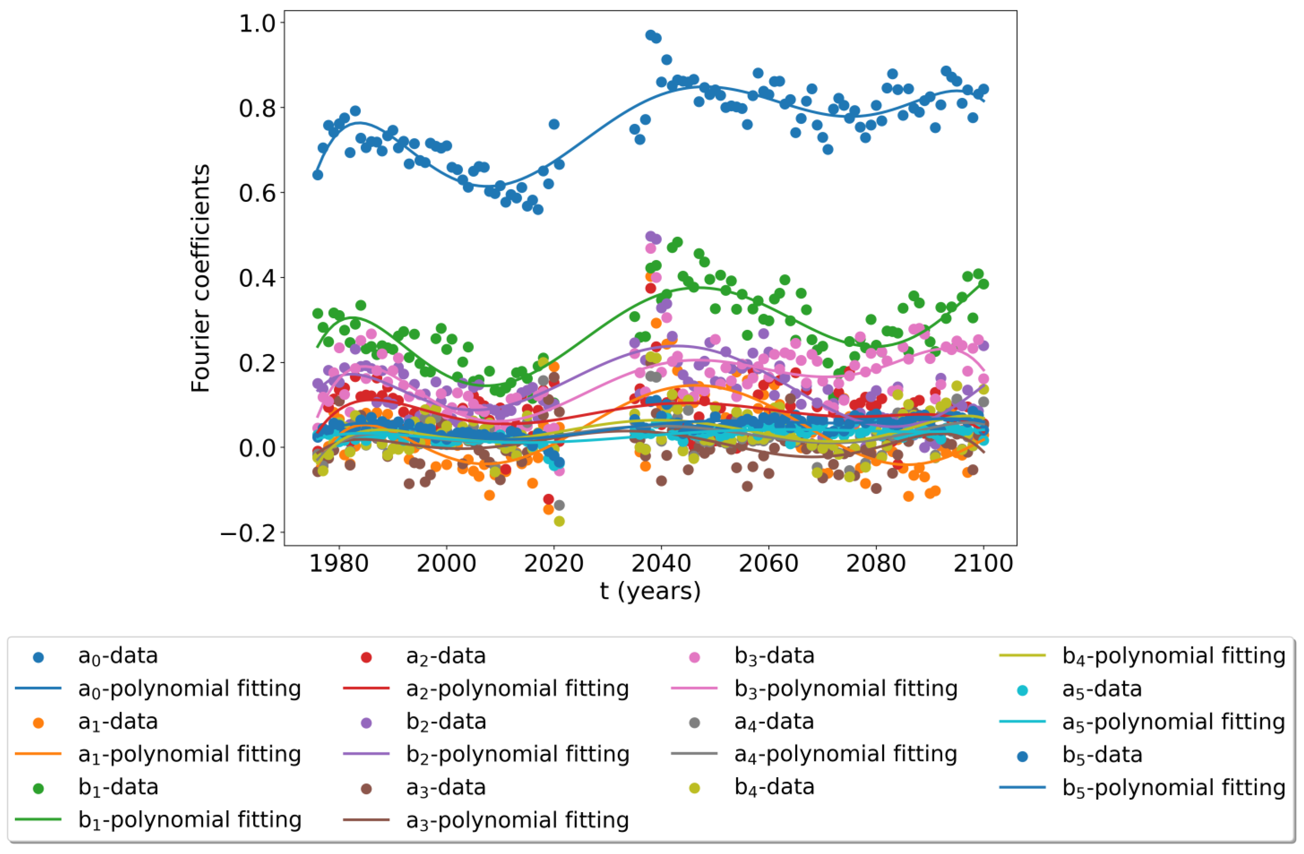
2.3.4. Trend Analysis in the NS-DEVA

As noted above, the directional model and its Fourier coefficients are estimated based on the data belonging to each time window $W_t$ at time step $t$. This process is followed by the polynomial fitting of a specific order to each Fourier coefficient of the GP location, scale, and shape parameter regarding the time. The polynomial order reveals the degree of data variability over time, so that a high polynomial order (usually more than 3) is needed to describe data presenting high variability over time. The polynomial trends are assessed through the ordinary least squares method, and the statistical significance of the polynomial terms has been examined using a t-test [64]. An analysis of variance (ANOVA) was then used to identify the simplest trend model among those with statistically significant terms (5% significance level) to provide an adequate description of the inherent trend in the Fourier series parameters. A similar approach was applied by Galiatsatou et al. [15], who used the t-test and an ANOVA to describe the inherent trend in the generalized extreme value distribution parameters for annual maximum values of $H_{m0}$.

It is worth mentioning that this step (see Figure 6) is performed to remove the short-term variability of the Fourier coefficients; consequently, the extreme wave climate patterns may lack statistical significance and should not be considered. Moreover, despite the gap in the data between the years 2017 and 2041, this is filled in the produced results through the polynomial fitting to the Fourier coefficient data, enabling their description via continuous functions of time.

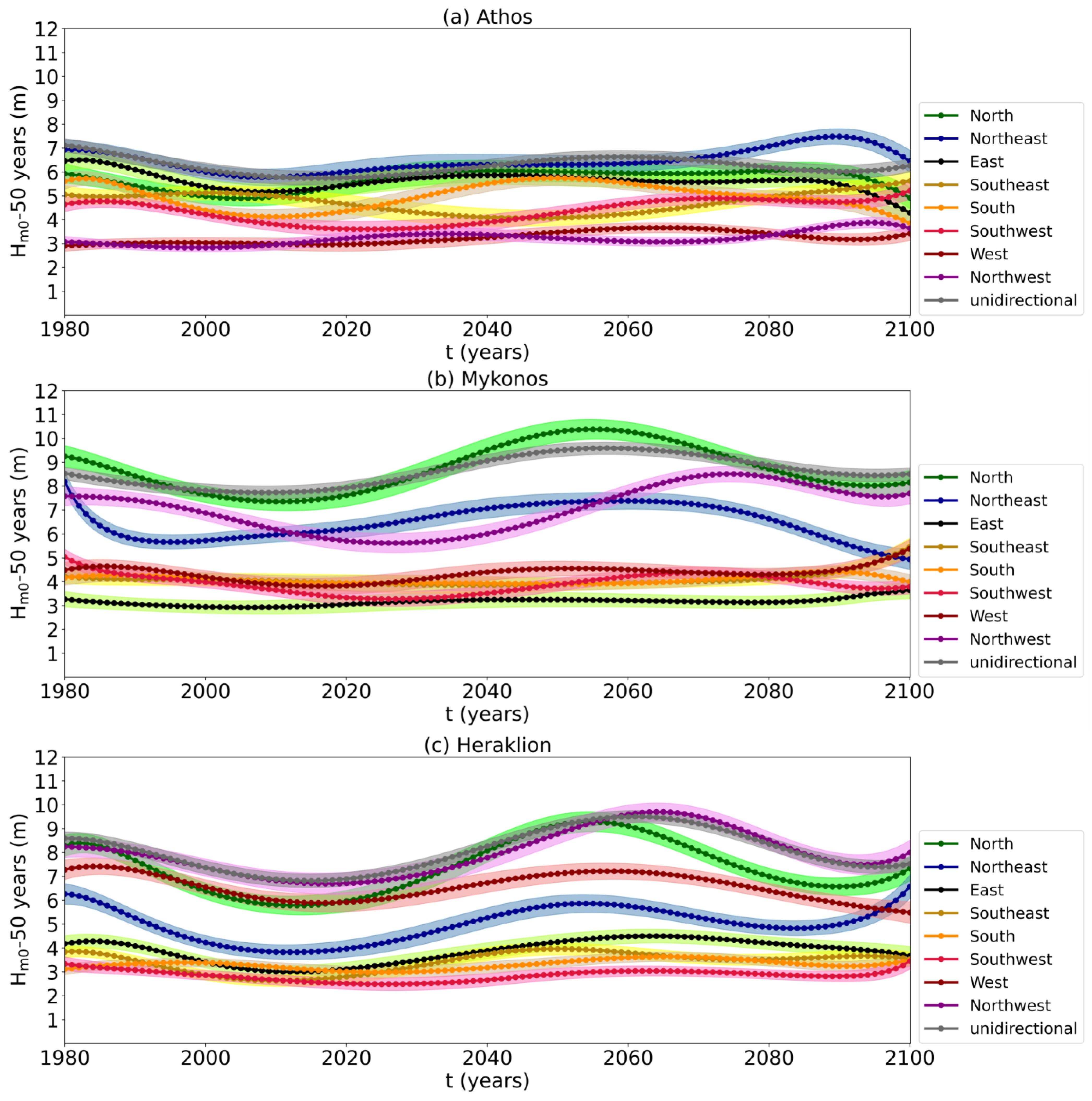
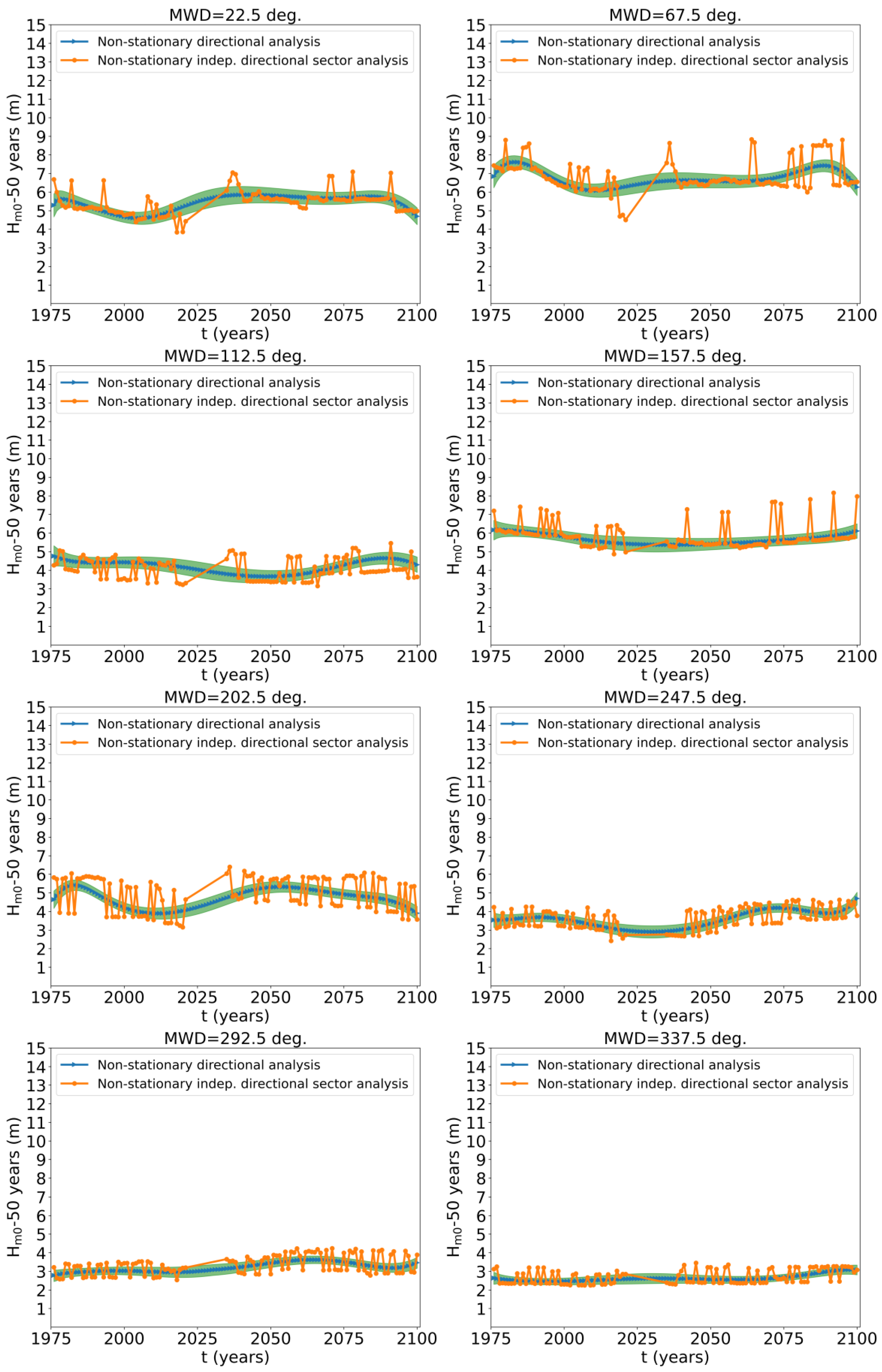
3. Results and Validation

A storm’s peak spectral significant wave height $H_{m0}$ corresponding to the return period of 50 years ($H_{m0}-50 \mathrm{y}\mathrm{e}\mathrm{a}\mathrm{r}\mathrm{s})$ is an indicative design return value for many marine and coastal applications. Thus, the sequences of $H_{m0}-50 \mathrm{y}\mathrm{e}\mathrm{a}\mathrm{r}\mathrm{s}$ associated to specific directions with respect to time (in years) we estimated (see Figure 7 and Figure 8) referring to the period from 1980 to 2100. Furthermore, the sequence of $H_{m0}-50 \mathrm{y}\mathrm{e}\mathrm{a}\mathrm{r}\mathrm{s}$ with respect to time in the unidirectional case, i.e., by ignoring the storms’ direction, was also estimated (see Figure 7 and Figure 8) in order to be compared with the directional results. It is also noted that the time-dependent $H_{m0}-50 \mathrm{y}\mathrm{e}\mathrm{a}\mathrm{r}\mathrm{s}$ estimates for all six areas were derived from the combination of a moving time window analysis, a directional model, and a trend analysis of the Fourier coefficients of the GP location, shape, and scale parameters of the directional model.

The Athos study area is mostly exposed to northeastern and eastern winds and wave storms, based on Figure 2 and Figure 7a, due to the geographical location of the Athos Peninsula and its coast orientation. All storms seem to have mild variations (i.e., up to ±12%) during the examined period ranging between 1980 and 2100. Nevertheless, the coastal storm patterns near Athos reveal a mild rise in northeastern extreme waves after the first half of the 21st century, notwithstanding a drop observed in $H_{\mathrm{m}0}$ extremes after 2090.

The time-dependent directional estimate of $H_{m0}-50 \mathrm{y}\mathrm{e}\mathrm{a}\mathrm{r}\mathrm{s}$ for the Mykonos case study reveals two prevailing directions of extreme coastal storms. These directions are northern and northeastern (see Figure 7b). Milder sea conditions correspond to other directions due to the shorter fetch lengths that result in less frequent and less intense coastal wave events. Coastal storms coming from north present a double peak during the period from 1980 to 2100. One peak can be observed around 1990, and the next one is likely to be observed around 2050. Moreover, the coastal storms from the northeastern direction are less intense over the examined period compared to those from the northern direction. The wave events from the other directions are likely to remain less severe with lower variation (up to ±10%) over the years compared to those from the north and northeast.

Referring to the Heraklion case study, although the location is in the southern Aegean, it is characterized by a similar northern $H_{m0}-50 \mathrm{y}\mathrm{e}\mathrm{a}\mathrm{r}\mathrm{s}$ profile to the Mykonos case study, since it has two peaks around 1990 and 2060 (see Figure 7c). Coastal storms coming from the northwest are also intense and are likely to be more severe than those from the north from 2080 to 2100. The extreme events coming from the other directions present milder variation among the years. Furthermore, a noticeable rise in $H_{m0}$ extremes from all examined directions can be observed in the [2020, 2070] time interval. Therefore, an increasing trend of coastal storm magnitudes can be observed in the middle of the 21st century.

The most intense coastal storms at the Rhodes interest point correspond to the eastern, southeastern, and southern directions, presenting low variations of up to ±10% (see Figure 8a). The severity of storms coming from southeastern and southern directions seems to stabilize after 2040, while the storms from the east show a drop from 2060 to 2090. After this period, the severity seems to intensify. The $H_{m0}$ extremes of the other directions are characterized by milder sea conditions compared to those of the eastern, southeastern, and southern directions.

Regarding the case study of Saronikos, three characteristic time periods can be observed for storms from the northern, northeastern, southeastern, southwestern, and northwestern directions (Figure 8b). The first period starts before than 1980 and ends in 2020, presenting a decreasing trend in terms of the storms’ magnitude. The second one ranges from 2020 to 2050, being characterized by an increasing trend, while the third one starts in 2050 and ends in 2100, presenting a decreasing trend. The coastal storms from the east, south, and west seem to intensify after 2090, notwithstanding the approximately similar pattern of $H_{m0}$ extremes for the other directions from 1980 to 2090.

The Pylos case study presents a wide range of storm severity values among the storms from different directions. This is attributed to the significantly different fetches for Pylos and the absence of islands from 160 degrees to 250 degrees from north, resulting in less wave diffraction. Hence, the most severe coastal storms are associated with the western, southwestern, and southern storm directions, presenting a decreasing trend from 1980 to 2020. An increasing trend is likely to appear between 2020 and 2040 for the western direction and between 2020 and 2070 for the southwestern and southern directions. This second peak is then followed by a severe decrease in the $H_{m0}-50 \mathrm{y}\mathrm{e}\mathrm{a}\mathrm{r} \mathrm{v}\mathrm{a}\mathrm{l}\mathrm{u}\mathrm{e}\mathrm{s}$ of up to 30% until 2100 for the western direction, while the storm profiles for southwestern and southern directions seem to stabilize. Additionally, the $H_{m0}$ extremes from the other directions have lower variation rates of up to 12% and appear milder than those corresponding to the western, southwestern, and southern directions (see Figure 8c).

The time-dependent directional results were validated by comparing them with those derived from the non-stationary independent sector analysis. Through these comparisons, it can be observed that the results follow the trends of the preliminary independent directional sector analysis by removing insignificant short-term variations of $H_{m0}-50 \mathrm{y}\mathrm{e}\mathrm{a}\mathrm{r} \mathrm{v}\mathrm{a}\mathrm{l}\mathrm{u}\mathrm{e}\mathrm{s}$. This was also confirmed by the application of the t-test [64] to the time sequences of $H_{m0}-50 \mathrm{y}\mathrm{e}\mathrm{a}\mathrm{r}\mathrm{s}$.

The validation process is presented for Athos (Figure 9) but was also applied for the five other case studies, although the results are not presented here for brevity.

4. Discussion

The time-dependent directional estimates of $H_{m0}$ extremes for the six examined locations were derived from a combination of a moving time window analysis, a simplified directional model, and a trend analysis of the Fourier coefficients of the GP location, shape, and scale parameters of the directional model.

The storms identification and representation process for each directional sector through the implementation of the three thresholds (see, e.g., [47,48]), namely the 0.95 quantile for $H_{m0}$, 6 h for the storm duration, and 12 h for the calm period between consecutive storms, as well as the use of the easy-to-apply automated $H_{m0}$ 0.95 quantile for the GP threshold, provides an adequate number of storms data for each directional sector. These adopted values for the three thresholds, when aiming to identify storm events, are in line with several research studies, such as [15,20,21]. Additionally, the non-parametric percentile or quantile method for $H_{m0}$ used here for the GP threshold value (e.g., [52,53]) can be applied to multiple datasets and locations [30].

Nevertheless, many research studies use either on a stationary or non-stationary unidirectional analysis, i.e., without considering the storm’s directionality as a covariate. On the contrary, in the present investigation, the identification and probabilistic representation of coastal storms were performed for each directional sector and incorporated into a time-dependent directional analysis. In the adopted approach, it was observed that in directional sectors with short fetch lengths, the mean rate of storm events was 1–3 per year, while in sectors with larger fetch lengths, this range was between 3 and 9 storms per year. Therefore, there was an adequate number of storm events for each directional sector and time window, so that the GP distribution represented them with satisfactory accuracy.

As for the directional dependence of the three GP parameters, this is often captured by means of a roughness-penalized ML estimation [30,34,62]. In this work, an alternative technique was utilized for the same purpose based on the basic theory of Fourier series expansion, avoiding the use of a roughness-penalized ML estimation for simplification. The adequate accuracy of this directional model was assured by using a simplified Fourier series expansion of the GP location, shape, and scale parameters and an optimization technique. The resulting overall accuracy of the directional model estimated by Equation (8) was satisfactory to a great degree for the six case studies (as seen in

Table 3. The overall accuracy of the directional model, estimated via Equation (8), associated with each examined interest point.

Interest Point	${\mathit{M}\mathit{A}\mathit{E}}_{\mathit{d}}$
Athos	0.0006 ± 0.0003
Mykonos	0.0007 ± 0.0005
Heraklion	0.0004 ± 0.0002
Rhodes	0.0002 ± 0.0001
Saronikos	0.0004 ± 0.0001
Pylos	0.0006 ± 0.0004

).

In addition, to remove the short-term and insignificant variability of the Fourier coefficients, a trend analysis was applied to these coefficients. As mentioned above, the polynomial trends were assessed through the ordinary least squares method. The statistical significance of the polynomial terms has been examined by using a t-test [64], in accordance with Galiatsatou et al. [15], who used a t-test and an ANOVA to describe the inherent trend in generalized extreme value distribution parameters for annual maximum values of $H_{m0}$. The selected polynomials ranged between 3 and 6 in all cases and for each Fourier coefficient.

Referring here to the results derived from the adopted non-stationary directional extreme value analysis (NS-DEVA), it was observed that in the Northern (Athos), Central (Mykonos), and Southern Aegean (Heraklion) and Ionian (Pylos) Seas, a considerable increase was detected in the extreme wave climate magnitude in the first half of the twenty-first century. In particular, this rise was most pronounced for the most severe storms that usually come from specific directions. Such storms are likely to be attenuated to some degree at the end of the twenty-first century. This finding is in line with [13,14,16,65], who studied the climate change effects on metocean conditions (storm surge and spectral wave characteristics) in selected areas of the eastern–central Mediterranean, Aegean, and Ionian Seas. Furthermore, for the second half of the twenty-first century, storminess attenuation was detected in directional sectors corresponding to the most severe storms, corroborating the climate change patterns of earlier studies [14,15,16,65].

The storminess attenuation at the end of twenty-first century derived from our results is also strengthened by several research studies. Specifically, according to Lionello et al. [10], milder wave storms were detected for 2071–2100 in the future A2 and B2 emission scenarios than for the present storms, except for the summer period in the central Mediterranean under the A2 scenario. Additionally, referring to the Italian coast and Adriatic Sea, Martucci et al. [11] and Benetazzo et al. [12] estimated a generally milder wave climate during the 2070–2099 future period, albeit with an estimated probable local intensification of coastal storms.

Regarding the examined unidirectional case (see Figure 7 and Figure 8), it was observed that the unidirectional estimates of $H_{m0}$ return values were more consistent with the directional estimates of higher storm intensity values as compared to the other directional sectors. Therefore, it is concluded that the unidirectional case could lead to an overestimation of a storm’s intensity to a significant directional range.

It can also be deduced from the present paper that coastal storms coming from directions of short fetches may present minor variations in their probability distributions over the years. Moreover, these storms are probably of a lower intensity than those coming from less fetch-limited directions, due to the greater wave diffraction effects in the first case. This was confirmed by similar findings such as those derived by Casas-Prat and Sierra [66], who investigated the present and future extreme wave climates of the Northwestern Mediterranean Sea. Furthermore, especially in the South Aegean Sea, based on [15], despite the Aeolian patterns after the first half of the twenty-first century being slightly intensified due to the complex dense insular nature of the Cyclades, the waves are prone to diffraction, leading to a slight decrease in $H_{m0}$ extremes.

5. Conclusions

In the present paper, a non-stationary directional extreme value analysis (NS-DEVA) was performed based on a moving time window analysis combined with an independent directional sector analysis and a directional extreme value model. The independent directional sector analysis was applied first and utilized to validate the results of the directional model. The directional model was applied to storm data at each time step. Its incorporation into the non-stationary directional extreme value analysis (NS-DEVA) enabled the probabilistic representation of coastal storms with respect to the time and direction by neglecting their short-term and insignificant variability.

Moreover, an alternative technique was utilized for the mathematical description of the directional model without using a roughness-penalized ML estimation. This technique is based on the basic theory of the Fourier series expansion, with some simplifications and an optimization process that improves the accuracy of the generalized Pareto parameter estimates.

The derived time-dependent directional results were validated by comparing them with those produced through the non-stationary independent sector analysis. The results followed the trends of the preliminary independent directional sector analysis by removing insignificant short-term variation in the storms’ significant wave heights.

Moreover, the results of this study seem to align with several studies focusing on the present and future extreme wave climates in the Eastern and Central Mediterranean. The most noteworthy results are as follows. The most likely and most extreme significant wave height estimates present a bimodal behavior with pronounced maxima. The first peak can be observed before the twenty-first century, i.e., around 1990, while the second peak is likely to occur around the middle of the twenty-first century for five of the examined locations, namely Mykonos, Heraklion, Rhodes, Saronikos, and Pylos. Storms coming from the northeast in the location of Athos seem to have their second peak around 2090, possibly because of the different location and orientation, and consequently this point is exposed to different wind and wave regimes compared to the rest of study areas. Moreover, coastal storms coming from directions of large fetches are the most severe storms, presenting a drop in their intensity at the end of the twenty-first century. On the contrary, coastal storms from fetch-limited directions may present minor variations in their probability distributions over the years.

In general, this paper presents an alternative technique for considering the storm direction as a covariate. Thus, coastal storms can be probabilistically represented from every direction over the directional domain, since their distribution (e.g., the generalized Pareto) parameters are expressed as functions of the direction via a simplified and easy-to-apply process. In addition, the coastal storms’ variability over the years and directions are considered in a unified, innovative approach, providing crucial information for various coastal engineering studies and wave energy applications. Furthermore, the adopted approach was applied to six characteristic locations in the Greek Seas in this paper but can be effectively implemented in every offshore and coastal location.

References

1. Solomon, S.; Qin, D.; Manning, M.; Chen, Z.; Marquis, M.; Averyt, K.B.; Tignor, M.; Miller, H.L. Intergovernmental Panel on Climate Change (IPCC). Climate change 2007: The scientifc basis. In Contribution of Working Group I to the Fourth Assessment Report of the Intergovernmental Panel on Climate Change; Cambridge University Press: New York, NY, USA, 2007. [Google Scholar]
2. Field, C.B.; Barros, V.; Stocker, T.F.; Dahe, Q.; Intergovernmental Panel on Climate Change (IPCC). Managing the risks of extreme events and disasters to advance climate change adaptation. In A Special Report of Working Groups I and II of the Inter-Governmental Panel on Climate Change; Cambridge University Press: Cambridge, UK, 2012. [Google Scholar]
3. Field, C.B.; Barros, V.R.; Dokken, D.J.; Mach, K.J.; Mastrandrea, M.D.; Intergovernmental Panel on Climate Change (IPCC). Climate change 2014: Impacts, adaptation and vulnerability. In Contribution of Working Group II to the Fifth Assessment Report of the Intergovernmental Panel on Climate Change; Cambridge University Press: Cambridge, UK, 2014. [Google Scholar]
4. Daneshfaraz, R.; Norouzi, R.; Ebadzadeh, P.; Di Francesco, S.; Abraham, J.P. Experimental Study of Geometric Shape and Size of Sill Effects on the Hydraulic Performance of Sluice Gates. Water 2023, 15, 314. [Google Scholar] [CrossRef]
5. Marcos, M.; Tsimplis, M.N. Coastal sea level trends in Southern Europe. Geophys. J. Int. 2008, 175, 70–82. [Google Scholar] [CrossRef] [Green Version]
6. Somot, S.; Sevault, F.; Déqué, M.; Crépon, M. 21st century climate change scenario for the Mediterranean using a coupled atmosphere-ocean regional climate model. Glob. Planet. Change 2008, 63, 112–126. [Google Scholar] [CrossRef] [Green Version]
7. Carillo, A.; Sannino, G.; Artale, V.; Ruti, P.M.; Calmanti, S.; Dell’Aquila, A. Steric sea level rise over the Mediterranean Sea: Present climate and scenario simulations. Clim. Dyn. 2012, 39, 2167–2184. [Google Scholar] [CrossRef]
8. Tsimplis, M.N.; Calafat, F.M.; Marcos, M.; Jordà, G.; Gomis, D.; Fenoglio-Marc, L.; Struglia, M.V.; Josey, S.A.; Chambers, D.P. The effect of the NAO on sea level and on mass changes in the Mediterranean Sea. J. Geophys. Res. Ocean. 2013, 118, 944–952. [Google Scholar] [CrossRef] [Green Version]
9. Adloff, F.; Somot, S.; Sevault, F.; Jordà, G.; Aznar, R.; Déqué, M.; Herrmann, M.; Marcos, M.; Dubois, C.; Padorno, E.; et al. Mediterranean Sea response to climate change in an ensemble of twenty first century scenarios. Clim. Dyn. 2015, 45, 2775–2802. [Google Scholar] [CrossRef]
10. Lionello, P.; Cogo, S.; Galati, M.B.; Sanna, A. The Mediterranean surface wave climate inferred from future scenario simulations. Glob. Planet. Change 2008, 63, 152–162. [Google Scholar] [CrossRef]
11. Martucci, G.; Carniel, S.; Chiggiato, J.; Sclavo, M.; Lionello, P.; Galati, M.B. Statistical trend analysis and extreme distribution of significant wave height from 1958 to 1999—An application to the Italian Seas. Ocean Sci. 2010, 6, 525–538. [Google Scholar] [CrossRef] [Green Version]
12. Benetazzo, A.; Fedele, F.; Carniel, S.; Ricchi, A.; Bucchignani, E.; Sclavo, M. Wave climate of the Adriatic Sea: A future scenario simulation. Nat. Hazards Earth Syst. Sci. 2012, 12, 2065–2076. [Google Scholar] [CrossRef] [Green Version]
13. Androulidakis, Y.S.; Kombiadou, K.D.; Makris, C.V.; Baltikas, V.N.; Krestenitis, Y.N. Storm surges in the Mediterranean Sea: Variability and trends under future climatic conditions. Dyn. Atmos. Ocean. 2015, 71, 56–82. [Google Scholar] [CrossRef]
14. Galiatsatou, P.; Anagnostopoulou, C.; Prinos, P. Modeling nonstationary extreme wave heights in present and future climates of Greek Seas. Water Sci. Eng. 2016, 9, 21–32. [Google Scholar] [CrossRef] [Green Version]
15. Galiatsatou, P.; Makris, C.; Prinos, P.; Kokkinos, D. Nonstationary joint probability analysis of extreme marine variables to assess design water levels at the shoreline in a changing climate. Nat. Hazards 2019, 98, 1051–1089. [Google Scholar] [CrossRef]
16. Makris, C.; Galiatsatou, P.; Tolika, K.; Anagnostopoulou, C.; Kombiadou, K.; Prinos, P.; Velikou, K.; Kapelonis, Z.; Tragou, E.; Androulidakis, Y.; et al. Climate change effects on the marine characteristics of the Aegean and Ionian Seas. Ocean Dyn. 2016, 66, 1603–1635. [Google Scholar] [CrossRef]
17. Makris, C.V.; Tolika, K.; Baltikas, V.N.; Velikou, K.; Krestenitis, Y.N. The impact of climate change on the storm surges of the Mediterranean Sea: Coastal sea level responses to deep depression atmospheric systems. Ocean Model. 2023, 181, 102149. [Google Scholar] [CrossRef]
18. Mazas, F.; Hamm, L. A multi-distribution approach to POT methods for determining extreme wave heights. Coast. Eng. 2011, 58, 385–394. [Google Scholar] [CrossRef]
19. Mazas, F. Extreme events: A framework for assessing natural hazards. Nat. Hazards 2019, 98, 823–848. [Google Scholar] [CrossRef]
20. Martzikos, N.T.; Prinos, P.E.; Memos, C.D.; Tsoukala, V.K. Statistical analysis of Mediterranean coastal storms. Oceanologia 2021, 63, 133–148. [Google Scholar] [CrossRef]
21. Martzikos, N.; Malliouri, D.; Tsoukala, V. Shape investigation and probabilistic representation of coastal storms. Applications to Mykonos and Barcelona. Appl. Ocean Res. 2023, 135, 103563. [Google Scholar] [CrossRef]
22. Malliouri, D.I.; Memos, C.D.; Soukissian, T.H.; Tsoukala, V.K. Assessing failure probability of coastal structures based on probabilistic representation of sea conditions at the structures’ location. Appl. Math. Model. 2021, 89, 710–730. [Google Scholar] [CrossRef]
23. Radfar, S.; Galiatsatou, P. Influence of nonstationarity and dependence of extreme wave parameters on the reliability assessment of coastal structures—A case study. Ocean Eng. 2023, 273, 113862. [Google Scholar] [CrossRef]
24. Radfar, S.; Shafieefar, M.; Akbari, H.; Galiatsatou, P.A.; Mazyak, A.R. Design of a rubble mound breakwater under the combined effect of wave heights and water levels, under present and future climate conditions. Appl. Ocean Res. 2021, 112, 102711. [Google Scholar] [CrossRef]
25. Malliouri, D.; Martzikos, N.; Tsoukala, V. Fully probabilistic reliability and resilience analysis of coastal structures based on damage evolution simulation. In Proceedings of the 39th IAHR World Congress, International Association for Hydro-Environment Engineering and Research (IAHR), Granada, Spain, 19–24 June 2022; pp. 5908–5916. [Google Scholar]
26. Tsoukala, V.K.; Chondros, M.; Kapelonis, Z.G.; Martzikos, N.; Lykou, A.; Belibassakis, K.; Makropoulos, C. An integrated wave modelling framework for extreme and rare events for climate change in coastal areas—The case of Rethymno, Crete. Oceanologia 2016, 58, 71–89. [Google Scholar] [CrossRef] [Green Version]
27. Gad, F.-K.; Chatzinaki, M.; Vandarakis, D.; Kyriakidou, C.; Kapsimalis, V. Assessment of Wave Storm-Induced Flood Vulnerability in Rhodes Island, Greece. Water 2020, 12, 2978. [Google Scholar] [CrossRef]
28. Dissanayake, P.; Brown, J.; Wisse, P.; Karunarathna, H. Effects of storm clustering on beach/dune evolution. Mar. Geol. 2015, 370, 63–75. [Google Scholar] [CrossRef]
29. Dissanayake, P.; Brown, J.; Sibbertsen, P.; Winter, C. Using a two-step framework for the investigation of storm impacted beach/dune erosion. Coast. Eng. 2021, 168, 103939. [Google Scholar] [CrossRef]
30. Karathanasi, F.; Soukissian, T.; Belibassakis, K. Directional Extreme Value Models in Wave Energy Applications. Atmosphere 2020, 11, 274. [Google Scholar] [CrossRef] [Green Version]
31. Coles, S.G. An Introduction to Statistical Modeling of Extreme Values; Springer: London, UK, 2001. [Google Scholar]
32. Mentaschi, L.; Vousdoukas, M.; Voukouvalas, E.; Sartini, L.; Feyen, L.; Besio, G.; Alfieri, L. The transformed-stationary approach: A generic and simplified methodology for non-stationary extreme value analysis. Hydrol. Earth Syst. Sci. 2016, 20, 3527–3547. [Google Scholar] [CrossRef] [Green Version]
33. Galiatsatou, P.; Makris, C.; Krestenitis, Y.; Prinos, P. Nonstationary Extreme Value Analysis of Nearshore Sea-State Parameters under the Effects of Climate Change: Application to the Greek Coastal Zone and Port Structures. J. Mar. Sci. Eng. 2021, 9, 817. [Google Scholar] [CrossRef]
34. Ewans, K.; Jonathan, P. The Effect of Directionality on Northern North Sea Extreme Wave Design Criteria. J. Offshore Mech. Arct. Eng. 2008, 130. [Google Scholar] [CrossRef]
35. Barlow, A.M.; Mackay, E.; Eastoe, E.; Jonathan, P. A penalised piecewise-linear model for non-stationary extreme value analysis of peaks over threshold. Ocean Eng. 2023, 267, 113265. [Google Scholar] [CrossRef]
36. Caires, S.; Yan, K. Ocean Surface Wave Time Series for the European Coast from 1976 to 2100 Derived from Climate Projections. Available online: https://cds.climate.copernicus.eu/cdsapp#!/dataset/sis-ocean-wave-timeseries?tab=overview (accessed on 1 January 2023).
37. Van Vuuren, D.P.; Edmonds, J.; Kainuma, M.; Riahi, K.; Thomson, A.; Hibbard, K.; Hurtt, G.C.; Kram, T.; Krey, V.; Lamarque, J.-F.; et al. The representative concentration pathways: An overview. Clim. Change 2011, 109, 5–31. [Google Scholar] [CrossRef]
38. Thomson, A.M.; Calvin, K.V.; Smith, S.J.; Kyle, G.P.; Volke, A.; Patel, P.; Delgado-Arias, S.; Bond-Lamberty, B.; Wise, M.A.; Clarke, L.E.; et al. RCP4.5: A pathway for stabilization of radiative forcing by 2100. Clim. Change 2011, 109, 77–94. [Google Scholar] [CrossRef] [Green Version]
39. Pielke, R., Jr.; Burgess, M.G.; Ritchie, J. Plausible 2005–2050 emissions scenarios project between 2 °C and 3 °C of warming by 2100. Environ. Res. Lett. 2022, 17, 024027. [Google Scholar] [CrossRef]
40. Höök, M.; Sivertsson, A.; Aleklett, K. Validity of the Fossil Fuel Production Outlooks in the IPCC Emission Scenarios. Nat. Resour. Res. 2010, 19, 63–81. [Google Scholar] [CrossRef] [Green Version]
41. Fisher, N.I. Statistical Analysis of Circular Data; Cambridge University Press: Cambridge, UK, 1995. [Google Scholar]
42. Arguez, A.; Vose, R.S. The Definition of the Standard WMO Climate Normal: The Key to Deriving Alternative Climate Normals. Bull. Am. Meteorol. Soc. 2011, 92, 699–704. [Google Scholar] [CrossRef] [Green Version]
43. Hirabayashi, Y.; Mahendran, R.; Koirala, S.; Konoshima, L.; Yamazaki, D.; Watanabe, S.; Kim, H.; Kanae, S. Global flood risk under climate change. Nat. Clim. Change 2013, 3, 816–821. [Google Scholar] [CrossRef]
44. Bender, J.; Wahl, T.; Jensen, J. Multivariate design in the presence of non-stationarity. J. Hydrol. 2014, 514, 123–130. [Google Scholar] [CrossRef]
45. Hipel, K.; McLeod, A. Time Series Modelling of Water Resources and Environmental Systems; Electronic Reprint of Our Book Originally Published in 1994; Elsevier: Amsterdam, The Netherlands, 2005. [Google Scholar]
46. Rutkowska, A. Properties of the Cox–Stuart Test for Trend in Application to Hydrological Series: The Simulation Study. Commun. Stat. Simul. Comput. 2015, 44, 565–579. [Google Scholar] [CrossRef]
47. Sanuy, M.; Duo, E.; Jäger, W.S.; Ciavola, P.; Jiménez, J.A. Linking source with consequences of coastal storm impacts for climate change and risk reduction scenarios for Mediterranean sandy beaches. Nat. Hazards Earth Syst. Sci. 2018, 18, 1825–1847. [Google Scholar] [CrossRef] [Green Version]
48. Duo, E.; Sanuy, M.; Jiménez, J.A.; Ciavola, P. How good are symmetric triangular synthetic storms to represent real events for coastal hazard modelling. Coast. Eng. 2020, 159, 103728. [Google Scholar] [CrossRef]
49. Langousis, A.; Mamalakis, A.; Puliga, M.; Deidda, R. Threshold detection for the generalized Pareto distribution: Review of representative methods and application to the NOAA NCDC daily rainfall database. Water Resour. Res. 2016, 52, 2659–2681. [Google Scholar] [CrossRef] [Green Version]
50. Davison, A.C.; Smith, R.L. Models for Exceedances Over High Thresholds. J. R. Stat. Soc. Ser. B 1990, 52, 393–425. [Google Scholar] [CrossRef]
51. Hall, W.; Weller, J. Mean residual life. In Statistics and Related Topics; Csorgo, M., Dawson, D.A., Rao, J.N.K., Saleh, A.K.M.E., Eds.; Norrh-Holland Publishing Company: Amsterdam, The Netherlands, 1981; pp. 169–184. [Google Scholar]
52. Eastoe, E.F.; Tawn, J.A. Modelling the distribution of the cluster maxima of exceedances of subasymptotic thresholds. Biometrika 2012, 99, 43–55. [Google Scholar] [CrossRef]
53. Grabemann, I.; Weisse, R. Climate change impact on extreme wave conditions in the North Sea: An ensemble study. Ocean Dyn. 2008, 58, 199–212. [Google Scholar] [CrossRef] [Green Version]
54. Benito, S.; López-Martín, C.; Navarro, M.Á. Assessing the importance of the choice threshold in quantifying market risk under the POT approach (EVT). Risk Manag. 2023, 25, 6. [Google Scholar] [CrossRef]
55. Papalexiou, S.M.; Koutsoyiannis, D.; Makropoulos, C. How extreme is extreme? An assessment of daily rainfall distribution tails. Hydrol. Earth Syst. Sci. 2013, 17, 851–862. [Google Scholar] [CrossRef] [Green Version]
56. Ochi, M.K. Ocean Waves—The Stochastic Approach; Cambridge University Press: Cambridge, UK, 1998. [Google Scholar]
57. Malliouri, D.I.; Memos, C.D.; Tampalis, N.D.; Soukissian, T.H.; Tsoukala, V.K. Integrating short- and long-term statistics for short-crested waves in deep and intermediate waters. Appl. Ocean Res. 2019, 82, 346–361. [Google Scholar] [CrossRef]
58. Hosking, J.R.M.; Wallis, J.R. Parameter and Quantile Estimation for the Generalized Pareto Distribution. Technometrics 1987, 29, 339–349. [Google Scholar] [CrossRef]
59. Moharram, S.H.; Gosain, A.K.; Kapoor, P.N. A comparative study for the estimators of the Generalized Pareto distribution. J. Hydrol. 1993, 150, 169–185. [Google Scholar] [CrossRef]
60. Castillo, E.; Hadi, A.S. Fitting the Generalized Pareto Distribution to Data. J. Am. Stat. Assoc. 1997, 92, 1609–1620. [Google Scholar] [CrossRef]
61. Robinson, M.E.; Tawn, J.A. Statistics for Extreme Sea Currents. J. R. Stat. Soc. Ser. C Appl. Stat. 1997, 46, 183–205. [Google Scholar] [CrossRef]
62. Green, P.J.; Silverman, B.W. Nonparametric Regression and Generalized Linear Models; Chapman and Hall/CRC: New York, NY, USA, 1993; ISBN 9780429161056. [Google Scholar]
63. Jonathan, P.; Ewans, K. The effect of directionality on extreme wave design criteria. Ocean Eng. 2007, 34, 1977–1994. [Google Scholar] [CrossRef]
64. Chambers, J. Chapter 4 of statistical models in S. In Linear Models; Chambers, J., Hastie, T., Eds.; Wadsworth & Brooks/Cole: Nashville, TN, USA, 1992. [Google Scholar]
65. Galiatsatou, P.; Prinos, P. Joint probability analysis of extreme wave heights and storm surges in the Aegean Sea in a changing climate. E3S Web Conf. 2016, 7, 02002. [Google Scholar] [CrossRef]
66. Casas-Prat, M.; Sierra, J.P. Projected future wave climate in the NW Mediterranean Sea. J. Geophys. Res. Ocean. 2013, 118, 3548–3568. [Google Scholar] [CrossRef]
Figure 1. Locations in the Eastern Mediterranean where wave climate data can be extracted from the Copernicus database (blue points) and the six examined locations (orange points).
Water 15 02455 g001
Figure 2. Rose diagrams of significant wave height and mean wave direction values.
Water 15 02455 g002
Figure 3. Brief description of the adopted NS-DEVA methodology.
Water 15 02455 g003
Figure 4. An example of the (5th Fourier order) directional model applied to the GP scale, shape, and location parameters with and without the use of the optimization technique, presented with respect to the storm MWD.
Water 15 02455 g004
Figure 5. Return values of H m 0 50   y e a r s (m) as a function of the storm MWD for the years 1990, 2000, 2075, and 2100, derived from the directional model.
Water 15 02455 g005
Figure 6. Polynomial fitting to the time-dependent Fourier coefficients of the GP scale parameter to remove short-term climate variability. Circles and lines of the same color refer to data and polynomial fitting of the same Fourier coefficient.
Water 15 02455 g006
Figure 7. Time-dependent directional estimates of H m 0 50   y e a r s and the unidirectional case for the Athos, Mykonos, and Heraklion case studies.
Water 15 02455 g007
Figure 8. Time-dependent directional estimates of H m 0 50   y e a r s and the directional case for the Rhodes, Saronikos, and Pylos case studies.
Water 15 02455 g008
Figure 9. Comparison and validation of the adopted methodology’s (NS-DEVA) results with those derived from the non-stationary independent sector directional analysis.
Water 15 02455 g009