Modeling Spatial Soil Water Dynamics in a Tropical Floodplain, East Africa

Abstract

Analyzing the spatial and temporal distribution of soil moisture is critical for ecohydrological processes and for sustainable water management studies in wetlands. The characterization of soil moisture dynamics and its influencing factors in agriculturally used wetlands pose a challenge in data-scarce regions such as East Africa. High resolution and good-quality time series soil moisture data are rarely available and gaps are frequent due to measurement constraints and device malfunctioning. Soil water models that integrate meteorological conditions and soil water storage may significantly overcome limitations due to data gaps at a point scale. The purpose of this study was to evaluate if the Hydrus-1D model would adequately simulate soil water dynamics at different hydrological zones of a tropical floodplain in Tanzania, to determine controlling factors for wet and dry periods and to assess soil water availability. The zones of the Kilombero floodplain were segmented as riparian, middle, and fringe along a defined transect. The model was satisfactorily calibrated (coefficient of determination; R² = 0.54–0.92, root mean square error; RMSE = 0.02–0.11) on a plot scale using measured soil moisture content at soil depths of 10, 20, 30, and 40 cm. Satisfying statistical measures (R² = 0.36–0.89, RMSE = 0.03–0.13) were obtained when calibrations for one plot were validated with measured soil moisture for another plot within the same hydrological zone. Results show the transferability of the calibrated Hydrus-1D model to predict soil moisture for other plots with similar hydrological conditions. Soil water storage increased towards the riparian zone, at 262.8 mm/a while actual evapotranspiration was highest (1043.9 mm/a) at the fringe. Overbank flow, precipitation, and groundwater control soil moisture dynamics at the riparian and middle zone, while at the fringe zone, rainfall and lateral flow from mountains control soil moisture during the long rainy seasons. In the dry and short rainy seasons, rainfall, soil properties, and atmospheric demands control soil moisture dynamics at the riparian and middle zone. In addition to these factors, depths to groundwater level control soil moisture variability at the fringe zone. Our results support a better understanding of groundwater-soil water interaction, and provide references for wetland conservation and sustainable agricultural water management.

1. Introduction

Analyzing the spatial and temporal distribution of soil moisture content is essential for understanding ecohydrological wetland processes and for the development of sustainable agricultural water management wetland studies [1,2]. Soil moisture content is an important variable in regulating and predicting a range of hydrological processes like flooding [3], plant water availability [4,5,6], and soil water-groundwater interaction [7]. Soil moisture content is equally crucial in the hydrological cycle for the estimation of the plot-catchment scale water balance [8]. Therefore, a better spatial and temporal assessment of soil moisture content yields valuable insights into hydrological processes and supports weather forecasting as well as climate projections [1,9,10].

Wetlands rely on water, whether derived from precipitation, surface, or sub-surface water, to fulfill their ecosystem functions such as nutrient retention, flood mitigation, and food provisioning through agricultural support [11,12]. Indeed, knowledge of hydrology is indispensable for wetland conservation and agricultural production [13,14,15]. In East Africa, floodplain wetlands are increasingly being utilized for agricultural production development projects, as a key intervention to synergistically achieve food security in the region [16]. This is due to their relatively large size, high soil nutrient stocks, and prolonged periods of soil water availability [17,18,19]. This is also evident for the floodplain wetland in the catchment of Kilombero river, the most important tributary of the Rufiji river basin, representing one of the largest basins of Tanzania. The catchment is, however, increasingly used for agricultural production, especially during periods of inundation in the long rainy season. According to References [20,21], rain-fed rice production has recently increased in the Kilombero floodplain. In fact, the wetland supplies about 9% of all rice produced in Tanzania. It is noteworthy that the Kilombero river catchment is also targeted for agricultural expansion through the project Southern Agricultural Growth Corridor Of Tanzania (SAGCOT) [22], a large-scale agricultural intensification project. In this context, assessment and an improved understanding of the amount and spatial dynamics of soil moisture is fundamental for crop growth, land use planning, and the evaluation of the potential impacts of agricultural management interventions on the hydrology and other ecosystem services of the floodplain.

Spatial and temporal soil moisture dynamics in floodplain wetlands are influenced by a range of factors; thus, assessing these factors through field observations is difficult and time-consuming. Soil moisture exhibits tremendous spatial heterogeneity even over small catchments, resulting from the interplay of hydrological, biological, and meteorological processes [23]. In order to better understand the spatial pattern of soil moisture for wetland conservation and land use planning, good-quality time series data is required. However, there is a paucity of reliable field-scale measured data, and the remotely sensed soil moisture data is too coarse in the spatial resolution and refers to 5-cm depth soil moisture [24]. Often, data gaps for the available soil moisture time series exist due to measurement constraints, device malfunctioning, or site inaccessibility during flooding periods. Moreover, during dry conditions, soil cracking affects the measuring moisture sensors and, therefore, data quality [25]. Statistical and data-driven methods are an option for filling in missing values in distributed soil moisture datasets. Alternatively, models that integrate meteorological conditions, soil water storage, land use, and depth to groundwater table [26] may significantly overcome data gaps at a point scale, which are inevitable under field conditions. Once these models are well calibrated and validated, assessment of the impacts of agricultural management on the ecosystem functioning of wetlands is feasible.

In this study, a widely used soil water model, Hydrus-1D [27], which simulates one-dimensional water, heat, and solute transport in variably saturated and unsaturated media, was applied to simulate the spatial soil moisture dynamics in the Kilombero floodplain. Models such as MODular Hydrologic Modelling System (MODHMS) [28], European Hydrological System (MIKE SHE) [29], and Hydrus-2D and -3D [30] can be adopted to simulate soil water dynamics. However, they are data demanding, require large computer resources, and are difficult to adapt to the investigated study area because of complex boundary conditions. Hydrus-1D, in comparison, is less data demanding and can easily be adopted at the local scale as well as at the East African regional scale, and has also been proven to be an effective tool for evaluating various water and solute fluxes in agricultural fields with different crops and various irrigation schemes [31,32]. Hydrus-1D has been successfully applied in numerous studies for predicting soil moisture content and movement under different conditions [33,34,35,36]. In spite of these previous efforts, there is still limited research on the assessment of the spatial soil moisture dynamics at the different hydrological zones of a tropical wetland using Hydrus-1D, especially for data-scarce tropical regions such as East Africa. Most of these studies [31,34,35,36] have been conducted in temperate regions, yet tropical regions continue to face data scarcity and quality challenges, especially in the recently degrading wetland ecosystems. The similarity of this study to previous works is the type of data (soil moisture content, depth to groundwater level, soil physical properties, leaf area index, and climatic data) used for model calibration and simulation of soil water dynamic and vertical fluxes. Many studies have described and explained the factors that influence soil water dynamics [6,37,38] and soil moisture retention [16,39,40] at the wetland-catchment scale in East Africa. However, these studies are tailored to inland valley wetlands, yet floodplain wetlands exhibit different hydrological behavior compared to the inland valley wetlands. Therefore, there is paucity of sufficient scientific information for proper floodplain wetland agricultural management planning in the region. This calls for more research on these floodplains to improve the scientific knowledge base for decision-making. The purpose of the study is to conduct a thorough study of the soil water dynamic based on field measurements so as to evaluate the agricultural usability of the different hydrological zones of the tropical floodplain wetland. This contributes to soil and land management as it provides the required scientific basis for decision-making and agricultural planning. Accordingly, the study has the following objectives (i) to test the applicability of the Hydrus-1D model for simulating spatial soil moisture content dynamics along different hydrological zones of the floodplain; (ii) to determine factors controlling soil moisture content dynamics at each hydrological zone during drying and wetting periods; and (iii) to assess soil water availability for each hydrological zone. In addition, a sensitivity analysis on selected water flux parameters, with varying depth to groundwater levels, was conducted for each hydrological zone. This was performed to understand how changes in groundwater levels, which may be caused by water extraction and catchment scale processes, will influence local water availability and water fluxes.

2. Materials and Methods

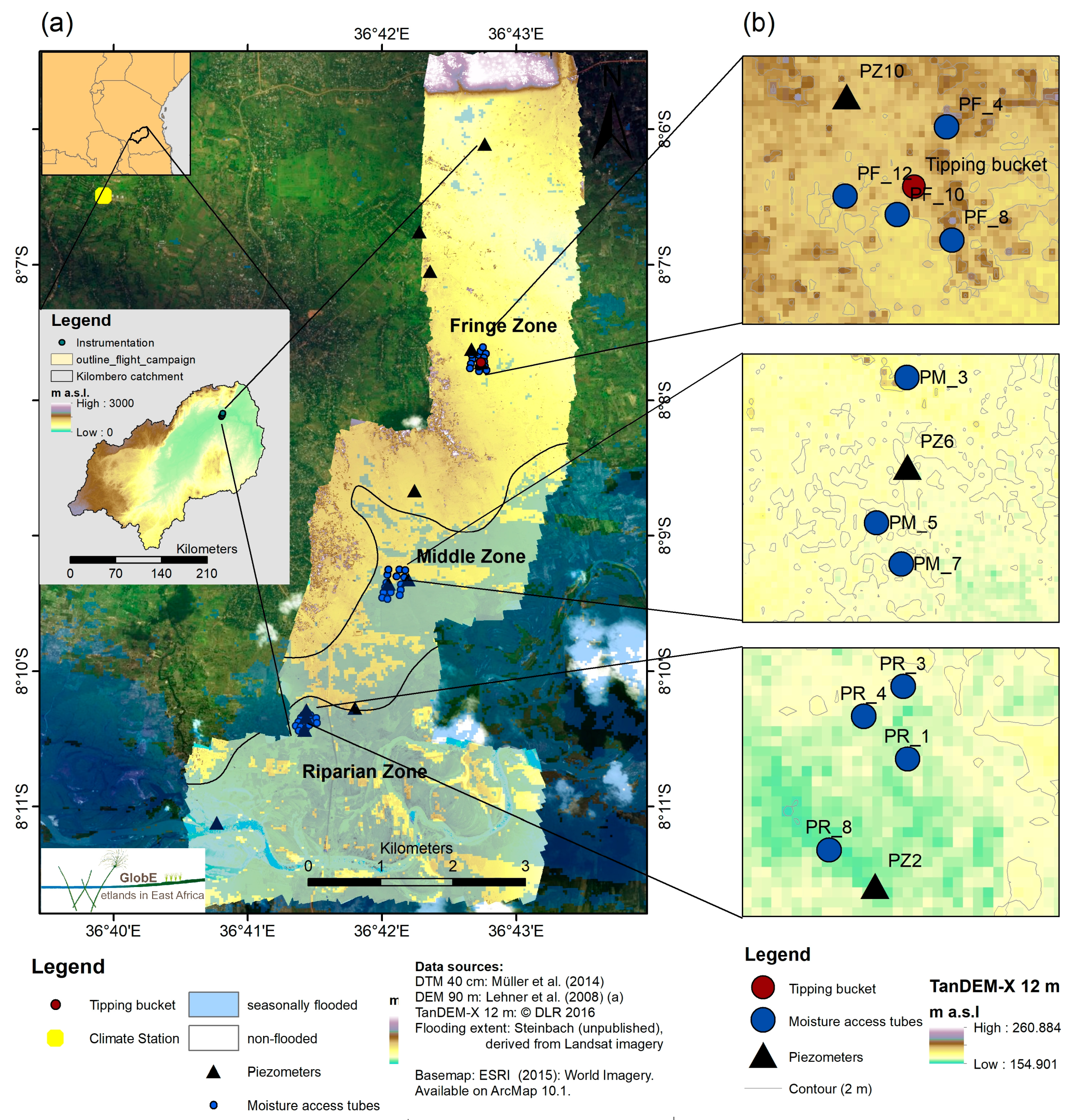
2.1. Study Area

The Kilombero floodplain wetland is part of the Rufiji basin and is situated in Kilombero and Ulanga districts, Morogoro region, southern Tanzania. The floodplain lies between latitudes 7.654° and 10.023° S and longitudes 34.563° and 37.797° E (Figure 1a), with elevation ranging from 250 to 300 m above sea level (a.s.l). The Kilombero catchment covers an area of 40,240 km², including the broad floodplain of the main Kilombero river with a spatial extent of about 7967 km² [41], in which the study area of about 96 km² is found (Figure 1). The floodplain is seasonally flooded and drained by the Kilombero river. The Kilombero river is an important tributary catchment of the Rufiji river basin, contributing 62% of the total annual average basin water flow [42]. A number of perennial and seasonal streams drain into the Kilombero River from the Udzungwa Mountains in the northwest and the Mahenge Mbarika escarpment in the southeast with elevation ranging from 200 to 2500 m a.s.l. [41,43].

The Kilombero floodplain is part of the Southern Agricultural Growth Corridor Of Tanzania (SAGCOT) [22], an area earmarked for future investments in agricultural development. The area forms a large triangle of some 500 km² that is bordered by three national parks. Besides a range of agro-industrial uses (mainly sugar cane), the cropped portion is dominated by rain-fed rice (wet season) and several irrigation schemes allowing for year-round irrigated rice production. In fact, the wetland supplies about 9% of all rice produced in Tanzania compared to the Mkomazi floodplain in the sub-humid lowlands west of Usambara Mountains. The area is characterized by diverse land uses, land use intensity gradients, and interactions between large- and small-scale crop farmers, landless herders, and urban populations.

The climate is sub-humid tropical with annual rainfall ranging from 1200 to 1400 mm and a mean annual temperature of about 23–25 °C [44]. The rainfall is distributed in a bi-modal structure. The long rainy season is from March to May, while the short rainy season spans from October to December [41]. The flood peaks are experienced mainly during the long rainy season, though they can also happen as early as January.

The geological substrate in the floodplain includes mainly a sedimentary basin, forming a seasonal alluvial floodplain dominated by Fluvisols soils [45]. However, according to Reference [46], sediments constitute alluvial fans, river deposits, and colluvial materials. The alluvial fans mark the transition between the floodplain and the fringes, with high infiltration rates and high soil moisture variability [46]. The soils tend to crack upon drying and experience ponding once the soil is swollen and cracks are closed. Within the study area, groundwater flow is directed from north to south towards Kilombero river throughout the year [46]. Groundwater recharge mainly occurs due to rainwater infiltration in the study area and the mountainous areas in the northern catchment.

The valley is predominantly characterized by Miombo woodlands, mainly Brachystegia species and grasses such as reed (Phragmites mauritianus), guinea grass (Panicum maximum), and elephant grass (Penisetum purpureum) [21]. Agriculture is the main economic activity in the valley. Agricultural production is practiced at both subsistence and commercial scales. Lowland rain-fed rice is the dominating food and cash crop cultivated in the valley; however, other crops such as maize and peas are grown, especially during the short rainy season.

2.2. Study Design

The valley was subdivided into three hydrological zones (riparian, middle, and fringe, see Figure 1a) based on the origin of flooding water, its extent, and duration. In total, 462 Landsat 7 Enhanced Thematic Mapper Plus (ETM+) and eight Operational Land Imager (OLI) surface reflectance images [47,48] across six tiles from the years 2013 to 2015 with a cloud coverage <80% were processed. Their multi-temporal statistical values were classified in a Random Forest approach to delineate riverine flooded areas and generate inundation extents for seasonally flooded zones during the long rainy season (Figure 1a). The non-flooded zone was defined as fringe, characterized by precipitation- and groundwater table-induced flooding [49]. The middle zone is partially flooded, whereas the riparian zone is nearly completely flooded during the long rainy season. Further spatial differentiation of the hydrological zones included the application of the TerraSAR-X digital elevation model with a resolution of 12 m (TanDEM-X-12 m) to derive the absolute height and the distance from the river [50]. The lower parts of the transect are flooded longer and with a higher water depth, thus the riparian zone was close to the river with a lower absolute height altitude (Figure 1a).

2.3. Hydrological Data Monitoring

Hydrological data variables were monitored for a period of 17 months (March 2015–June 2016).

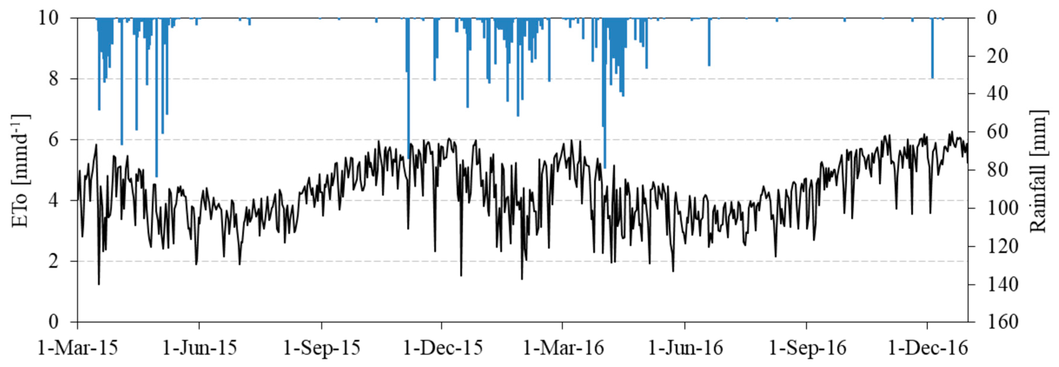
2.3.1. Meteorological Data

Daily rainfall values were measured in a tipping bucket rain gauge with a 0.2-mm resolution [51], installed at the fringe zone of the floodplain (Figure 1). Temperature, relative humidity, wind speed, and solar radiation were obtained from an automatic weather station situated close to the study area (Figure 1a).

2.3.2. Soil Moisture and Groundwater Level Monitoring

Soil moisture measurements were conducted at the three defined hydrological zones. At each hydrological zone, at least four soil moisture access tubes (Figure 1b) were installed for a Frequency-Domain-Reflectometry (FDR) profile probe type PR2 [52] to measure soil moisture content every two days. Other moisture measurement devices such as soil Hydra probe sensors [51], decagon 5TE soil moisture sensors [53], Theta probes, and tensiometers can be adopted for field soil moisture measurements. In this study, the profile probe used was a portable device which takes simultaneous measurements at depths of 10, 20, 30, and 40 cm within the access tube. The FDR profile probe type PR2 was used to measure the profile soil moisture up to soil depths of 40 cm and 100 cm, consisting of a sealed polycarbonate rod with a diameter of about 25 mm, electronic sensors arranged at fixed intervals along its length, and presenting a measurement accuracy of ±0.06 m³/m³ at 0 to 40 °C under generalized soil calibration in normal soils [52]. FDR is based on a unique relation between the volumetric water content and the dielectric constant of mineral soils. According to References [25,54,55], a Delta-T profile probe shows measurement difficulties in high clay soils; however, results are improved with site-specific calibration. In this study, site-specific calibrations were not conducted since the calibration of FDR sensors to tropical wetland soil conditions have been established by Reference [37], who approved their applicability with an error of 0.07 m³/m³. Therefore, the measured moisture results from the probes are reliable for tropical wetland conditions. Soil moisture readings were manually recorded with a handheld (HH2) moisture meter connected to a profile probe sensor [56].

To monitor the depth to groundwater level in the study area, three 10-cm-diameter piezometer pipes were installed, one at each hydrological zone (Figure 1b). The depth to groundwater level was measured hourly using pressure data loggers [57] installed in the piezometers.

2.3.3. Soil Properties Sampling

Soil physical properties were characterized at each installed access tube. Composite soil samples were collected at depths of 10, 20, 30, and 40 cm using a soil auger to analyze the soil particle size distribution and soil organic carbon (SOC). Soil particle size distribution was measured using the laser method [58], while SOC was determined using the modified Blackley Walkley wet method [59]. Three undisturbed soil samples (250 cm³) for each sampled soil depth were taken at each site for saturated hydraulic conductivity (K_sat) measurements using the constant head method with a laboratory permeameter [60]. Bulk density was determined with the core method using the same samples as those employed for the saturated hydraulic conductivity. These soil properties were used to drive the model setup and calibration.

2.4. Simulation of Soil Water Dynamics

2.4.1. Model Description

Simulations of soil water dynamics were performed using the Windows-based one-dimensional Hydrus-1D v4.09 software package [27] developed by PC-Progress s.r.o in Czech Republic. The model simulates variably saturated-unsaturated water flow by numerically solving Richard’s equation [61]:

$$\frac{\partial \theta }{\partial t}=\frac{\partial }{\partial x}\left[K\left(h\right)\left(\frac{\partial h}{\partial x}+1\right)\right]-S\left(h\right)$$

(1)

where θ is the volumetric soil water content (L³/L³), t is time (T), x is the vertical space coordinate (L), K is the hydraulic conductivity, h is the water pressure head (L), and S (h) is a water sink term accounting for root water uptake (L³/(L³·T)). Unsaturated soil hydraulic properties were represented by the parameterization given by [62]:

$$\theta \left(h\right)=\{\begin{array}{c}{\theta }_r+\frac{{\theta }_s-{\theta }_r}{{\left[1+{|\alpha h|}^n\right]}^m}h<0\\ {\theta }_{s}h\ge 0\end{array}$$

(2)

$$K\left(h\right)=K_{s }{S}_e{}^l{\left[{\left(1-S_e{}^{1/m}\right)}^m\right]}^2$$

(3)

$$S_e=\frac{\theta -{\theta }_r}{{\theta }_s-{\theta }_r}$$

(4)

where θ_r and θ_s are residual and saturated water contents (L³/L³), respectively, K_s is the saturated hydraulic conductivity (L/T¹), S_e is the effective saturation, α (L⁻¹), and l and n represent empirical shape parameters (the inverse air–entry point, pore connectivity, and pore-size distribution parameter, respectively), m = 1 − 1/n.

The sink term S (h) in Equation (1) is defined as the volume of water derived from a unit volume of soil per unit time by plant roots. It accounts for actual root water uptake equivalent to actual transpiration, calculated by the model using Feddes equation [63]:

$$S\left(h\right)=\alpha \left(h\right)S_p$$

(5)

where α (h) is the root water uptake stress response function, and S_p is a potential root water uptake rate (T⁻¹). Root water uptake is assumed to be zero close to saturation (i.e., wetter than the “anaerobiosis point”, h₁), and dryer than the wilting point pressure head (h₄). Root water uptake is considered to be at optimum between pressure heads h₂ and h₃, while root water uptake increases (or decreases) linearly with h when the pressure heads are between h₃ and the wilting point (or between h₂). Potential root water uptake is equal to root water uptake rate during periods of no water stress (when α (h) = 1).

2.4.2. Initial and Boundary Conditions

The initial conditions in the model were set to pressure heads in equilibrium with the measured depth to groundwater level, which was taken as a lower boundary condition. When the water table was above the soil surface, the pressure head was fixed to full saturation to facilitate modeling. The upper boundary condition was specified as an atmospheric boundary condition with a surface layer (to permit water build-up due to flooding) using daily rainfall, potential evapotranspiration, and leaf area index (LAI). Potential evapotranspiration (ET_p) was calculated by the Food and Agriculture Organization (FAO) Penman-Monteith equation [64]. A number of methods, for example, the water balance method [65], the Priestley-Taylor method [66], the Bowen-ratio method [67], and the Hargreaves equation [68], can be used for the calculation of potential evapotranspiration. According to Reference [64], the FAO Penman-Monteith method is physically based and can be used to predict ET_p in a wide range of locations and climates, even in data-scarce situations like Sub-Saharan Africa. The method uses meteorological data such as maximum and minimum temperature, relative humidity, wind speed, and solar radiation. These data were obtained from the automatic weather station located within the study site. Time series for meteorological conditions used for the simulation period are depicted in Figure 2. Actual evaporation and transpiration were directly computed by the model based on the given soil moisture conditions and root water uptake functions.

Leaf area index (LAI) values were measured at different growth stages of rain-fed lowland rice using a LI-COR area meter, an indirect method. Direct methods like the planimetrical approach and the gravimetric procedure can be used, but are time-consuming and destructive [69]. The LI-COR area meter is fast and uses a fisheye lens to project a nearly hemispheric image of the canopy and sky onto a ringed detector. This enables quick measurement of the leaf area index and foliage orientation over a large area [69]. In this study, LAI values were linearly interpolated between the measurement dates to obtain time series values.

2.4.3. Model Calibration and Validation

The model was calibrated for one year (March 2015 to March 2016), by comparing the simulated and field-measured daily soil moisture content at the different soil depths (10, 20, 30, and 40 cm), and different plots for each hydrological zone. Plots PR_1, PR_3, PR_4, and PR_8 for the riparian zone, PM_3, PM_5, and PM_7 for the middle zone, and PF_4, PF_8, PF_10, and PF_12 for fringe zone were used for calibration (Figure 1b). The one-year period included the drying and wetting conditions, allowing us to fit the model at a wide range of soil moisture conditions in the floodplain. The soil material layer/horizon was defined in accordance with depth intervals used for monitoring soil moisture content in a profile of 200 cm. A profile of 200 cm was defined because the observed groundwater table is within this range.

Hydrus-1D was calibrated using site-specific boundary conditions and field-measured soil moisture content. Van Genuchten hydraulic parameters, which describe the soil retention and unsaturated hydraulic conductivity functions, were optimized through inverse modeling with no hysteresis. In the Hydrus-1D model, inverse parameter estimation employs a relatively simple, gradient-based, local optimization algorithm based on the Marquardt-Levenberg method [27]. The aim of this method is to determine the best estimate of the hydraulic model parameters [61]. Hydraulic parameters estimated via the Rosetta pedotransfer functions [70] using measured soil particle size distribution (percentage clay, silt, and sand) and bulk density were used as initial estimates, in addition to the measured saturated hydraulic conductivity (

Table 1. Measured soil physical properties at the three hydrological zones of the floodplain.

Hydrological Zone	Soil Depth	BD	Ksat	SOC	Clay	Silt	Sand	Texture Class
	cm	(g/cm3)	(cm/d)	%
Riparian	10	1.03	114.50	1.88	35.02	56.18	8.80	Silty clay loam
	20	1.21	38.00	1.43	36.44	48.06	15.50	Silty clay loam
	30	1.27	17.13	0.83	34.27	37.87	27.86	Clay loam
	40	1.28	19.38	0.59	29.50	35.84	34.66	Clay loam
Middle	10	1.43	116.94	1.36	18.84	58.27	22.89	Silt loam
	20	1.33	120.57	1.56	21.58	61.92	16.50	Silt loam
	30	1.39	33.91	1.11	20.9	56.21	22.89	Silt loam
	40	1.38	27.62	0.91	29.4	56.17	14.43	Silty clay loam
Fringe	10	1.27	174.05	1.42	13.89	57.25	28.86	Silt loam
	20	1.36	180.93	1.39	14.20	59.07	26.73	Silt loam
	30	1.36	305.00	1.13	15.39	60.30	24.32	Silt loam
	40	1.39	101.01	0.99	15.86	58.37	25.77	Silt loam

BD; bulk density, K_sat; saturated hydraulic conductivity, SOC; soil organic carbon.

). Alpha, n, and saturated water content parameters were fitted first, since the Hydrus-1D model could optimize only 15 parameters at a time. Residual water content and the L parameter were the last to be estimated. The values of K_sat were reviewed and re-adjusted accordingly.

During the rice growing period, Feddes’ parameters for the tropical climate were taken from [71]: h₁ = 100 cm, h₂ = 55 cm, h₃ = −160 cm, h₄ = −250 cm, h₄ = −16,000 cm and the root distribution with a maximum of 40 cm were specified according to Reference [72]. After rice harvest (i.e., during the dry and the short rainy seasons, in which the sites were under fallow), we used the Feddes’ parameters for grass implemented in Hydrus-1D.

The calibrated model from each plot was validated for one year, with measured soil moisture data for the neighboring plots at each hydrological zone. The aim of this approach was to test the transferability of the calibrated model to predict spatial soil moisture for sites with similar biophysical properties and climate conditions. At each hydrological zone, two calibrated plots were validated with measured moisture data of the neighboring plots. At the riparian zone, plot PR_1 and PR_4 were validated with measured soil moisture data from plot PR_3 (88 m distant) and PR_1 (75 m distant), respectively. At the middle zone, plot PM_3 and PM_7 were validated with measured soil moisture values from plot PM_7 (400 m distant) and plot PM_5 (102 m distant), respectively. At the fringe, plot PF_10 and PF_8 were validated with measured soil moisture data from plot PF_12 (109 m distant), and PF_4 (225 m distant), respectively (Figure 1b).

2.4.4. Criterion for Model Calibration Performance

The agreement between predicted and observed moisture data was evaluated by (i) the coefficient of determination (R²); (ii) the Nash-Sutcliffe model efficiency coefficient (NSE); and (iii) the root mean square error (RMSE). Kling-Gupta efficiency (KGE) [73] and percent bias (PBIAS) [74] are other evaluation approaches which can be used for evaluating model quality. In this study, we used R², NSE, and RMSE. R² describes the proportion of the variance in measured data explained by the model. R² ranges from 0 to 1, with values greater than 0.5 considered to be acceptable [75]. The NSE is a dimensionless quality measure used to determine the relative magnitude of the residual variance between the simulated and measured data variance [76]. NSE ranges between −∞ and 1.0. An NSE of 1.0 indicates a perfect fit between the simulated and observed data [75]. RMSE is an error index statistic which measures the difference between simulated and observed values. The lower the RMSE, the better the performance of the model.

$${\mathrm{R}}^2=\frac{{[{{\displaystyle \sum }}_{i=1}^n(O_i-\overline{O})(P_i-\overline{P})]}^2}{{{\displaystyle \sum }}_{i=1}^n{(O_i-\overline{O})}^2{{\displaystyle \sum }}_{i=1}^n{(P_i-\overline{P})}^2}$$

(6)

$$\mathrm{NSE}=1-\frac{{{\displaystyle \sum }}_{i=1}^n{\left(O_i-P_i\right)}^2}{{{\displaystyle \sum }}_{i=1}^N{\left(O_i-\overline{O}\right)}^2}$$

(7)

$$\mathrm{RMSE}=\sqrt{\frac{{{\displaystyle \sum }}_{i=1}^n{\left(O_i-P_i\right)}^2}{n}}$$

(8)

where $O_i$ and $P_i$ are the observed and predicted moisture values, respectively, $\overline{O}$ and $\overline{P}$ are the mean of observed and predicted moisture values, and n is the number of observations.

2.5. Sensitivity Analysis

A sensitivity analysis was performed to analyze the impact of changes in the depth to groundwater level (dgwl) on root water uptake, evaporation, and change in soil water storage parameters. Evapotranspiration (transpiration and evaporation) is the major cause of water loss in the wetlands [36,77], while soil water storage is the most important state variable for crop growth. Therefore, understanding the impact of changes in the depth to groundwater level is essential to assess the water balance of the study area for sustainable agricultural and wetland management planning. Considering data for one year (July 2015–June 2016) as a reference, the mean dgwl was increased and decreased by 15%, 30%, 45%, and 60%. To evaluate the sensitivity of each parameter, the sensitivity index (SI) for each percentage change in dgwl was calculated according to de Roo (1993) cited in [78]:

$$\mathrm{SI}=\frac{\left|P_i-P_m\right|}{P}$$

(9)

With P_i = model output with a 15%, 30%, 45%, and 60% increase in the mean dgwl; P_m = model output with a related 15%, 30%, 45%, and 60% decrease in the mean dgwl; P = model output with base dgwl.

A number of sensitivity analysis methods exist, for example, variance-based methods, correlation and regression analysis methods, and Monte Carlo methods [79]. We used the sensitivity index method for this study because of its simplicity and because the sensitivity is clearly attributed to one model parameter.

3. Results

3.1. Simulation of Spatial Soil Water Dynamics at Different Scales

Hyrus-1D was set up, calibrated, and validated at the riparian, middle, and fringe hydrological zones of the floodplain.

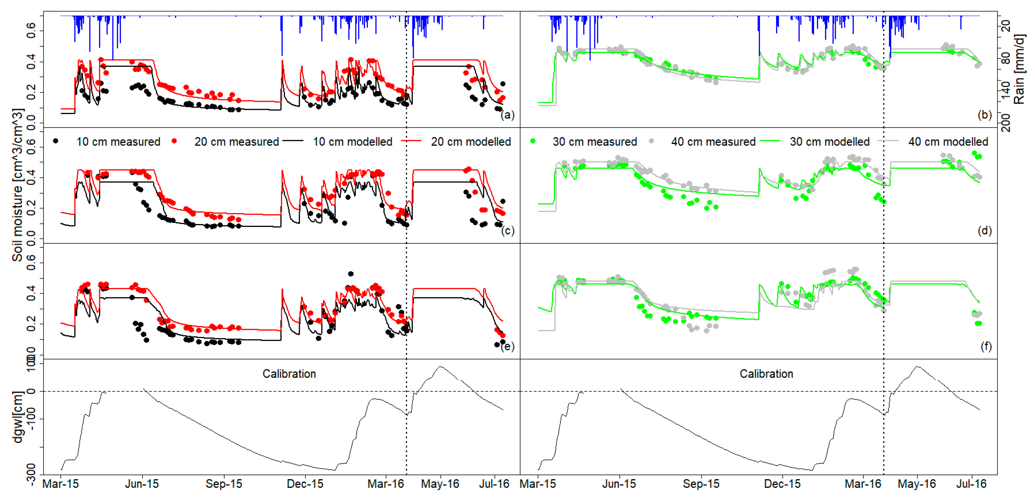
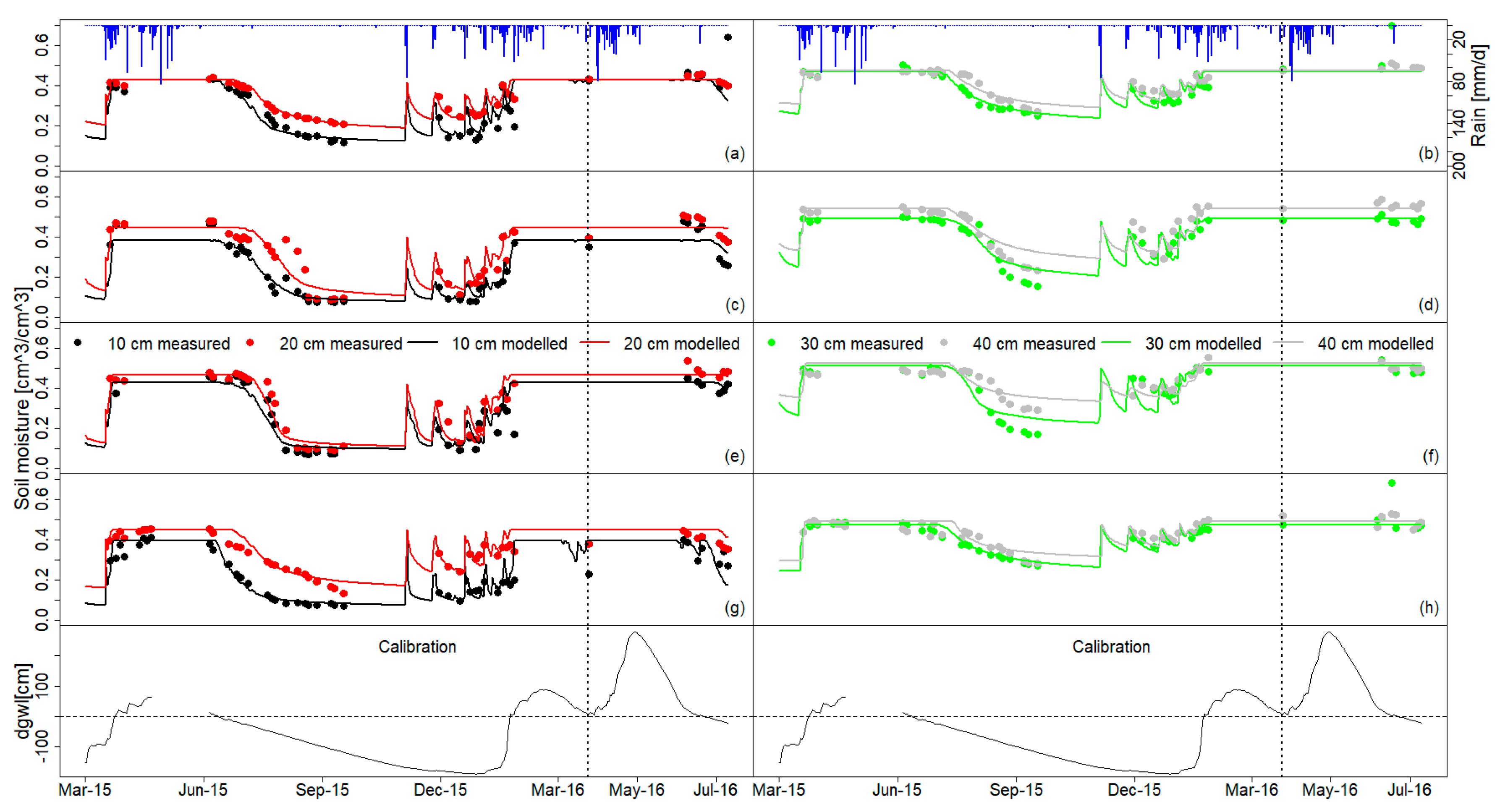
3.1.1. Calibration Results

A comparison of model performances and quality of statistical measures are presented in

Table 2. Statistical measures of the Hydrus-1D model performance for simulations of soil moisture content at the riparian zone after calibration.

Statistic Measure	Soil Depth (cm)
	10	20	30	40
Plot PR_4
R2	0.78	0.88	0.73	0.83
NSE	0.77	0.87	0.73	0.83
RMSE (cm3/cm3)	0.06	0.03	0.05	0.03
Plot PR_1
R2	0.90	0.81	0.82	0.70
NSE	0.89	0.80	0.82	0.70
RMSE (cm3/cm3)	0.04	0.06	0.05	0.06
Plot PR_8
R2	0.40	0.88	0.80	0.67
NSE	0.37	0.88	0.79	0.63
RMSE (cm3/cm3)	0.14	0.05	0.05	0.04
Plot PR_3
R2	0.85	0.89	0.92	0.76
NSE	0.79	0.81	0.91	0.74
RMSE (cm3/cm3)	0.05	0.04	0.02	0.03

for the riparian zone. Time series soil moisture content was well captured by the model for the four calibrated individual plots. A good agreement between modeled and observed soil moisture content as indicated by high R² (0.67–0.92), NSE (0.63–0.91), and low RMSE (0.03–0.06) was obtained (Table 2).

The best fit of van Genuchten hydraulic parameters for each plot is shown in

Table 3. Calibrated van Genuchten hydraulic parameters for the different plots at the riparian zone of the floodplain.

Soil Depth (cm)	Plot	θr (cm3/cm3)	θs (cm3/cm3)	α (cm−1)	n	Ksat (cm/d)	l
10	PR_4	0.08	0.43	0.05	2.00	78.87	0.50
	PR_1	0.06	0.38	0.03	2.500	738.5	0.68
	PR_8	0.08	0.43	0.03	2.98	300	0.50
	PR_3	0.04	0.39	0.13	1.83	609.15	0.45
20	PR_4	0.11	0.43	0.04	1.95	7.95	0.22
	PR_1	0.05	0.45	0.02	2.66	171.8	0.13
	PR_8	0.08	0.47	0.03	2.86	214	0.5
	PR_3	0.09	0.45	0.05	2.18	3.50	0.07
30	PR_4	0.1	0.47	0.04	1.66	209.8	0.12
	PR_1	0.1	0.49	0.02	2.40	323.6	0.7
	PR_8	0.08	0.51	0.02	2.11	6.53	0.5
	PR_3	0.12	0.47	0.05	1.78	12.08	0.01
40	PR_4	0.1	0.47	0.06	1.42	7.27	0.5
	PR_1	0.09	0.54	0.03	1.57	6.24	1.2
	PR_8	0.08	0.52	0.07	1.28	7.84	0.5
	PR_3	0.12	0.49	0.13	1.36	6.2	0.23

. The calibrated hydraulic parameters showed slight differences among the plots at soil depths of 10, 20, 30, and 40 cm. The final calibrated saturated hydraulic conductivity was higher than the measured values (Table 1 and Table 3).

Soil moisture content dynamics for both the rainy and dry seasons were well reproduced by the model for all of the soil layers. Measured and modeled soil moisture content values increased with soil depth. Flooding from both river overbank flow and local rainfall occurred during the long rainy season (March to May) and in the months of January to February 2016, which experienced heavy rains, correlated to El Niño–Southern Oscillation (ENSO) [80,81] and the Indian Ocean zonal mode (IOZM) [82].

At the riparian zone, the depth to groundwater level increased on average up to 1.6 m above the soil surface during the long rainy seasons; thus, the soils were fully saturated. During these periods, the model was able to reproduce soil moisture content trends and showed constant values (indicating soil saturation) until the floods receded (Figure 3). During flood recession (when the depth to groundwater level increased below the surface i.e., after June 2015), both modeled and measured soil moisture content showed a similar decreasing trend. For the short rainy season, the depth to groundwater level continued to increase below the surface until it reached 150 cm. Interestingly, measured and modeled soil moisture content at the different soil depths responded positively to rainfall events. Therefore, rainfall controlled soil moisture dynamics during this period (Figure 3). In addition, soil moisture dynamics could be explained by the differences observed in calibrated hydraulic parameters along the soil depths. The calibrated soil hydraulic parameters showed slight differences among the plots by visual comparison (Table 3). Thus, within the hydrological zones, there were relatively similar soil moisture patterns among the plots. This was depicted in the measured and modeled soil moisture content for the individual plots in the riparian zone, which showed almost similar trends throughout the different seasons (Figure 3).

Figure 4 presents the time series measured depth to groundwater level and calibration results of soil moisture content at the middle hydrological zone of the floodplain. Results revealed that the modeled soil moisture content exhibited variation tendencies quite similar to the measured data at the different soil depths in all of the plots. Modeled and measured soil moisture content increased with increase in soil depth.

Overall, there was a good agreement between modeled and measured soil moisture content after calibration (R² = 0.59–0.89, NSE = 0.51–0.88, and RMSE = 0.02–0.10 cm³/cm³) (

Table 4. Statistical measures of the Hydrus-1D model performance for simulations of soil moisture content at the middle zone after calibration.

Statistic Measure	Soil Depth (cm)
	10	20	30	40
Plot PM_3
R2	0.76	0.82	0.82	0.88
NSE	<<0	0.71	0.82	0.88
RMSE (cm3/cm3)	0.07	0.04	0.03	0.02
Plot PM_5
R2	0.65	0.88	0.87	0.89
NSE	0.63	0.87	0.72	0.87
RMSE (cm3/cm3)	0.09	0.04	0.05	0.03
Plot PM_7
R2	0.59	0.84	0.74	0.88
NSE	0.51	0.85	0.77	0.71
RMSE (cm3/cm3)	0.10	0.04	0.05	0.06

). The best fit of the van Genuchten hydraulic parameters for individual plots are shown in

Table 5. Calibrated van Genuchten hydraulic parameters for the different plots at the middle zone of the floodplain.

Soil Depth (cm)	Plot	θr (cm3/cm3)	θs (cm3/cm3)	α (cm−1)	n	Ksat (cm/d)	l
10	PM_3	0.04	0.37	0.08	1.85	85.4	0.49
	PM_5	0.04	0.37	0.03	1.7	128	0.49
	PM_7	0.04	0.37	0.03	1.53	65.72	0.48
20	PM_3	0.06	0.41	0.07	1.91	21.45	0.41
	PM_5	0.06	0.45	0.06	1.46	100	0.41
	PM_7	0.06	0.43	0.04	1.38	150	0.42
30	PM_3	0.04	0.46	0.02	1.8	0.93	0.0002
	PM_5	0.04	0.46	0.04	1.35	0.55	0.0002
	PM_7	0.04	0.46	0.01	1.36	2.49	0.002
40	PM_3	0.03	0.48	0.04	1.72	3.04	3.36
	PM_5	0.03	0.50	0.03	1.54	2.34	3.36
	PM_7	0.03	0.48	0.14	1.35	5.08	3.32

. There was almost no difference observed between the calibrated hydraulic parameters among the plots, except for saturated hydraulic conductivity. Hence, small variations between the modeled and measured soil moisture content values were noted among the plots.

The depth to groundwater level at the middle hydrological zone increased up to approximately 100 cm above the soil surface, causing full saturation of the soil layers during the long rainy season (March–June) (Figure 4). In the dry and short rainy seasons, the depth to groundwater level gradually declined up to 300 cm below the surface. Moreover, the model was capable of simulating the seasonal soil moisture content variations. During the short rainy season, both simulated and measured soil moisture content strongly responded to rainfall events in spite of the continued declining depth to groundwater level (Figure 4). Therefore, rainfall and soil properties played an important role in controlling soil moisture dynamics during dry and short rainy seasons at the middle zone. Modeled soil moisture dynamics during this period were well captured, except for some plots in which the simulated soil moisture showed high amplitude from the measured soil moisture content. Overall, the simulations were in agreement with the measurements.

Figure 5 and

Table 6. Statistical measures of the Hydrus-1D model performance for simulations of soil moisture content at the fringe zone after calibration.

Statistic Measure	Soil Depth (cm)
	10	20	30	40
Plot PF_8
R2	0.68	0.73	0.54	0.47
NSE	<<0	0.35	0.11	0.34
RMSE (cm3/cm3)	0.08	0.06	0.10	0.11
Plot PF_10
R2	0.87	0.85	0.85	0.74
NSE	0.85	0.82	0.85	0.73
RMSE (cm3/cm3)	0.05	0.03	0.03	0.02
Plot PF_4
R2	0.84	0.82	0.85	0.80
NSE	0.83	0.09	0.44	<<0
RMSE (cm3/cm3)	0.04	0.08	0.06	0.08
Plot PF_12
R2	0.82	0.73	0.67	0.58
NSE	0.33	0.47	0.67	0.58
RMSE (cm3/cm3)	0.04	0.03	0.04	0.03

show the calibrated results of soil moisture and model performance, respectively at the fringe zone of the floodplain. The modeled soil moisture content depicted a trend relatively similar to the measured soil moisture over time at the 10-cm depth intervals among the plots. The R² among the calibrated plots varied from 0.54 to 0.87, RMSE ranged from 0.03 to 0.11 cm³/cm³, and NSE varied from <0 to 0.85 (Table 6). Although modeled values were satisfactory, the model somewhat over- and underestimated soil moisture content at all of the plots (Figure 5).

Likewise, the calibrated van Genuchten hydraulic parameters showed slight variations at 10-cm depth intervals within and across the individual plots. This could be due to the low heterogeneity in soil texture (clay, sand, and silt content) and bulk density within the fringe position. Saturated hydraulic conductivity greatly varied along the four soil depths within and across the plots (

Table 7. Calibrated van Genuchten hydraulic parameters from the different plots at the fringe zone of the floodplain.

Soil Depth (cm)	Plot	θr (cm3/cm3)	θs (cm3/cm3)	α (cm−1)	n	Ksat (cm/d)	l
10	PF_12	0.09	0.28	0.002	1.56	28.4	0.26
	PF_10	0.08	0.38	0.05	2.5	64.2	0.5
	PF_4	0.08	0.35	0.04	2.5	24.62	0.5
	PF_8	0.08	0.35	0.002	1.35	24.62	0.5
20	PF_12	0.03	0.36	0.002	1.16	1.76	0.5
	PF_10	0.03	0.4	0.02	1.7	48.6	0.5
	PF_4	0.03	0.4	0.02	2.2	1.1	0.5
	PF_8	0.03	0.37	0.006	1.27	1.1	0.5
30	PF_12	0.04	0.41	0.1	1.19	1.3	0.05
	PF_10	0.05	0.41	0.03	2.36	65.2	0.5
	PF_4	0.05	0.41	0.03	2.1	1.3	0.5
	PF_8	0.05	0.41	0.08	1.32	1.92	0.5
40	PF_12	0.15	0.4	0.08	1.53	10.8	0.07
	PF_10	0.09	0.45	0.05	1.36	12.54	0.5
	PF_4	0.09	0.46	0.05	1.34	18.46	0.5
	PF_8	0.09	0.4	0.1	1.64	6.13	0.5

), which can be explained by the effect of soil macrospores, the cracking, and the occurrence of slickensides as a consequence of swell-and-shrink behavior, which were commonly encountered in clay-rich horizons during sampling.

Modeled and measured soil moisture time series showed a positive response to rainfall events, although high dynamics were observed during the wetting and drying periods (October to December 2016) for all of the soil depths across the plots. The monitored plots were flooded for a short time during the rainy season (March to June during the study) and in the short heavy rains (January to February 2016) (Figure 5). The depth to groundwater level gradually increased up to approximately 50 cm above the soil surface, saturating the soil layers. Thereafter, the depth to groundwater level declined to approximately 120 cm below the surface during the dry season (July to September 2015). However, in comparison to the riparian and middle zones, the variations in the depth to groundwater level were lower at the fringe zone. Equally important, the model was able to capture the seasonal soil moisture variability at the different plots amidst the existing data gaps in the measured soil moisture content. Also, the discrepancies between the simulated and measured soil moisture time series at the fringe were not different from those observed at the riparian and middle zones across the calibrated plots. Unlike at the riparian and middle zones, the depth to groundwater level and soil moisture content exhibited a positive response to single rainfall events during the wetting and drying periods (October to December 2016) at the fringe zone. Thus, the depth to groundwater level, rainfall, and soil properties control soil moisture dynamics at this zone.

Additionally, we tested the hypothesis that the model can simulate soil moisture dynamics averaged from individual plots, after aggregating the plot-specific calibrated hydraulic parameters within the hydrological zone. Therefore, the calibrated van Genuchten hydraulic parameters for each plot from the respective hydrological zones were averaged at each soil depth (

Table 8. Averaged calibrated hydraulic parameters at each hydrological zone.

Hydrological Zone	Soil Depth	θr (cm3/cm3)	θs (cm3/cm3)	α (cm−1)	n	Ksat (cm/d)	l
Riparian zone	10	0.07	0.41	0.06	2.33	431.63	0.53
	20	0.08	0.45	0.04	2.41	99.31	0.23
	30	0.10	0.49	0.03	1.99	138.00	0.33
	40	0.10	0.51	0.07	1.41	6.88	0.61
Middle zone	10	0.04	0.37	0.05	1.69	93.04	0.49
	20	0.06	0.43	0.06	1.58	90.48	0.41
	30	0.04	0.46	0.02	1.50	1.32	0.0009
	40	0.03	0.49	0.07	1.54	3.49	3.35
Fringe zone	10	0.08	0.34	0.02	1.98	35.46	0.44
	20	0.03	0.38	0.01	1.58	13.14	0.5
	30	0.05	0.41	0.06	1.74	17.43	0.39
	40	0.11	0.43	0.07	1.47	11.98	0.39

).

The Hydrus-1D model was set up with these averaged hydraulic parameters to simulate soil moisture content for each hydrological zone. The simulations were evaluated by comparing the modeled soil moisture content with the averaged measured soil moisture content at 10-cm depth increments. Figure 6 shows the typical results.

Overall, the modeled soil moisture time series showed good agreement with the averaged measured soil moisture content. There were some discrepancies between the modeled and measured soil moisture content values. This could be explained by the low variations in the hydraulic parameters observed at each individual plot of the respective hydrological zones. Generally, the model performance was good at the different hydrological zones. For example, R² varied from 0.78 to 0.90, NSE = 0.74–0.87, and RMSE ranged from 0.03 to 0.06 at the riparian zone; at the middle zone, R² = 0.62–0.90, NSE = 0.54–0.86, and RMSE = 0.03–0.06; and for the fringe zone, R² = 0.75–0.82, RMSE = 0.03–0.07, and NSE ranged from 0.37 to 0.75 (

Table 9. Hydrus-1D performance for soil moisture simulation after using averaged hydraulic parameters calculated from all of the calibrated plots for each hydrological zone.

Soil Depth (cm)	Riparian Zone			Middle Zone			Fringe Zone
	R2	NSE	RMSE	R2	NSE	RMSE	R2	NSE	RMSE
10	0.78	0.74	0.06	0.62	0.54	0.06	0.75	0.37	0.07
20	0.90	0.87	0.04	0.89	0.86	0.03	0.75	0.42	0.05
30	0.90	0.87	0.03	0.90	0.86	0.03	0.82	0.37	0.05
40	0.82	0.79	0.03	0.90	0.86	0.03	0.80	0.75	0.03

).

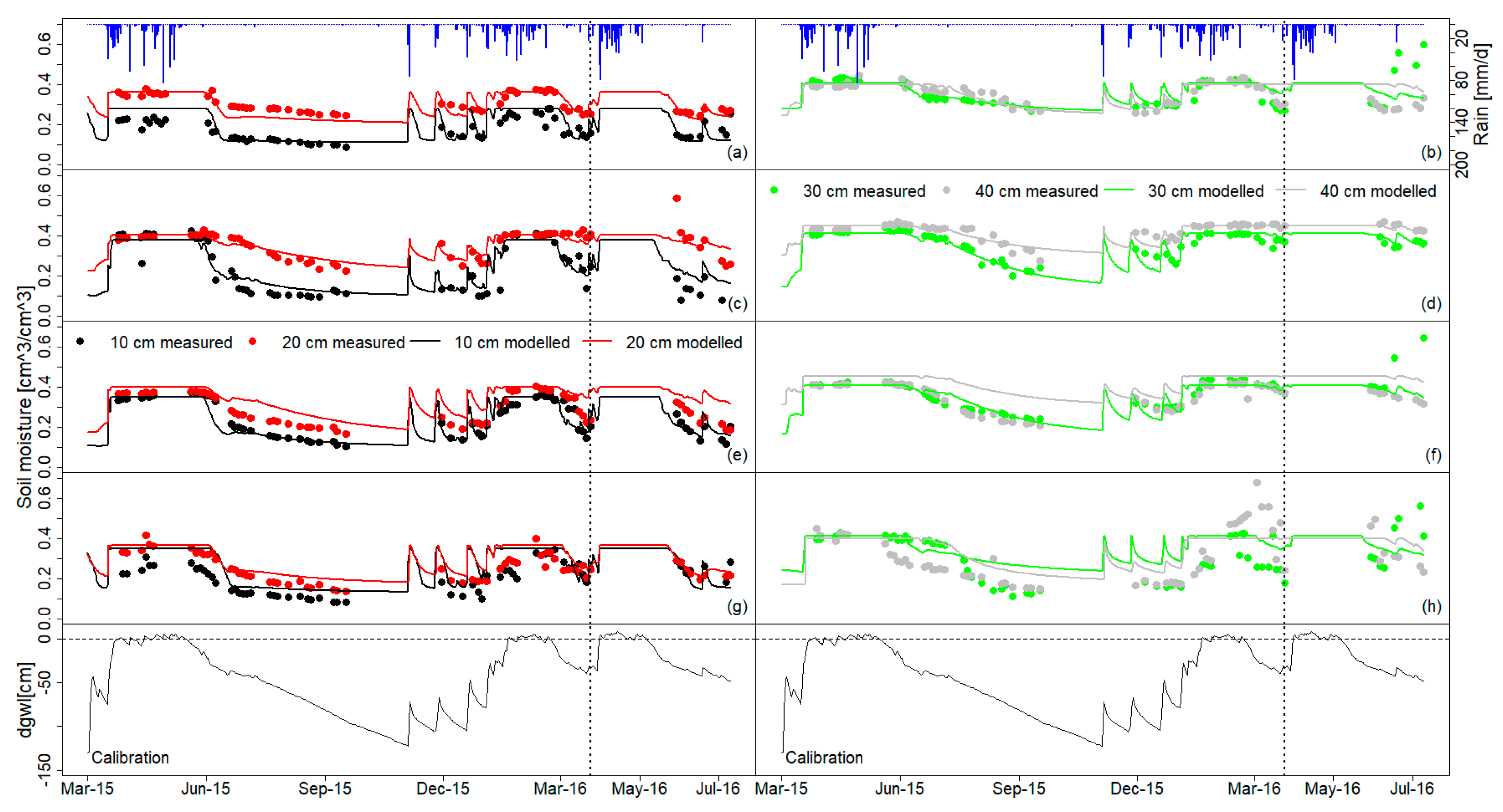
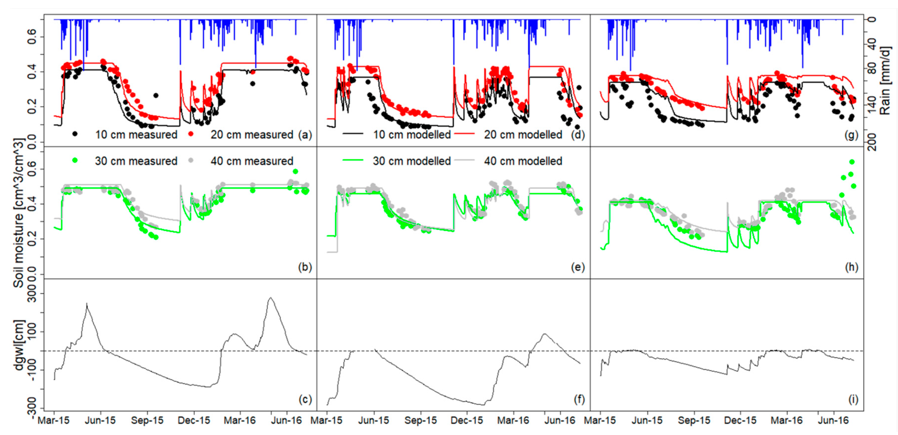
3.1.2. Validation Results and Prediction of Spatial Soil Moisture Content

We randomly validated the calibrated plots against the neighboring plots with measured soil moisture content data at soil depths of 10 and 30 cm for each hydrological zone. In doing so, we were able to test the transferability of model parameters calibrated at one plot to predict spatial soil moisture dynamics of another plot located in the same hydrological zone. As expected, model accuracy was higher for calibration than validation. Nevertheless, the modeled results are reasonable with low variability against the measured soil moisture content at each plot along the different soil depths by visual comparison (Figure 7). Validation resulted in R² = 0.64–0.89 and RMSE = 0.06–0.07 for the riparian zone; R² = 0.36–0.82 and RMSE = 0.07–0.13 for the middle zone; and R² = 0.52–0.91 and RMSE = 0.04–0.10 for the fringe zone (

Table 10. Hydrus-1D performance for soil moisture simulation after validation.

Hydrological Zone	Statistic Measure	Soil Depth (cm)
		10	20	30	40
Riparian	Plot PR_4 vs. PR_1
	R2	0.89	0.79	0.77	0.80
	NSE	0.80	0.69	0.74	0.49
	RMSE (cm3/cm3)	0.06	0.07	0.05	0.07
	Plot PR_1 vs. PR_3
	R2	0.79	0.75	0.64	0.65
	NSE	0.68	0.42	0.14	0.07
	RMSE (cm3/cm3)	0.07	0.07	0.09	0.06
Middle	Plot PM_5 vs. PM_7
	R2	0.36	0.84	0.69	0.61
	NSE	0.31	0.84	0.59	0.40
	RMSE (cm3/cm3)	0.13	0.05	0.07	0.09
	Plot PM_7 vs PM_3
	R2	0.63	0.76	0.82	0.87
	NSE	<<0	0.28	0.15	0.74
	RMSE (cm3/cm3)	0.11	0.07	0.13	0.03
Fringe	Plot PF_8 vs. PF_4
	R2	0.84	0.83	0.91	0.85
	NSE	0.81	0.53	0.46	0.84
	RMSE (cm3/cm3)	0.04	0.06	0.06	0.03
	Plot PF_10 vs. PF_12
	R2	0.81	0.63	0.52	0.61
	NSE	<<0	<<0	0.28	<<0
	RMSE (cm3/cm3)	0.10	0.06	0.05	0.07

). The goodness-of-fit values indicated satisfactory agreement between modeled values and field measurements for both rainy and dry seasons and demonstrated the acceptable accuracy of model simulations. Thus, the results supporting the hypothesis of the model’s feasibility to simulate spatial soil water dynamics within sites of similar topography, as well as other biophysical properties once it is well calibrated.

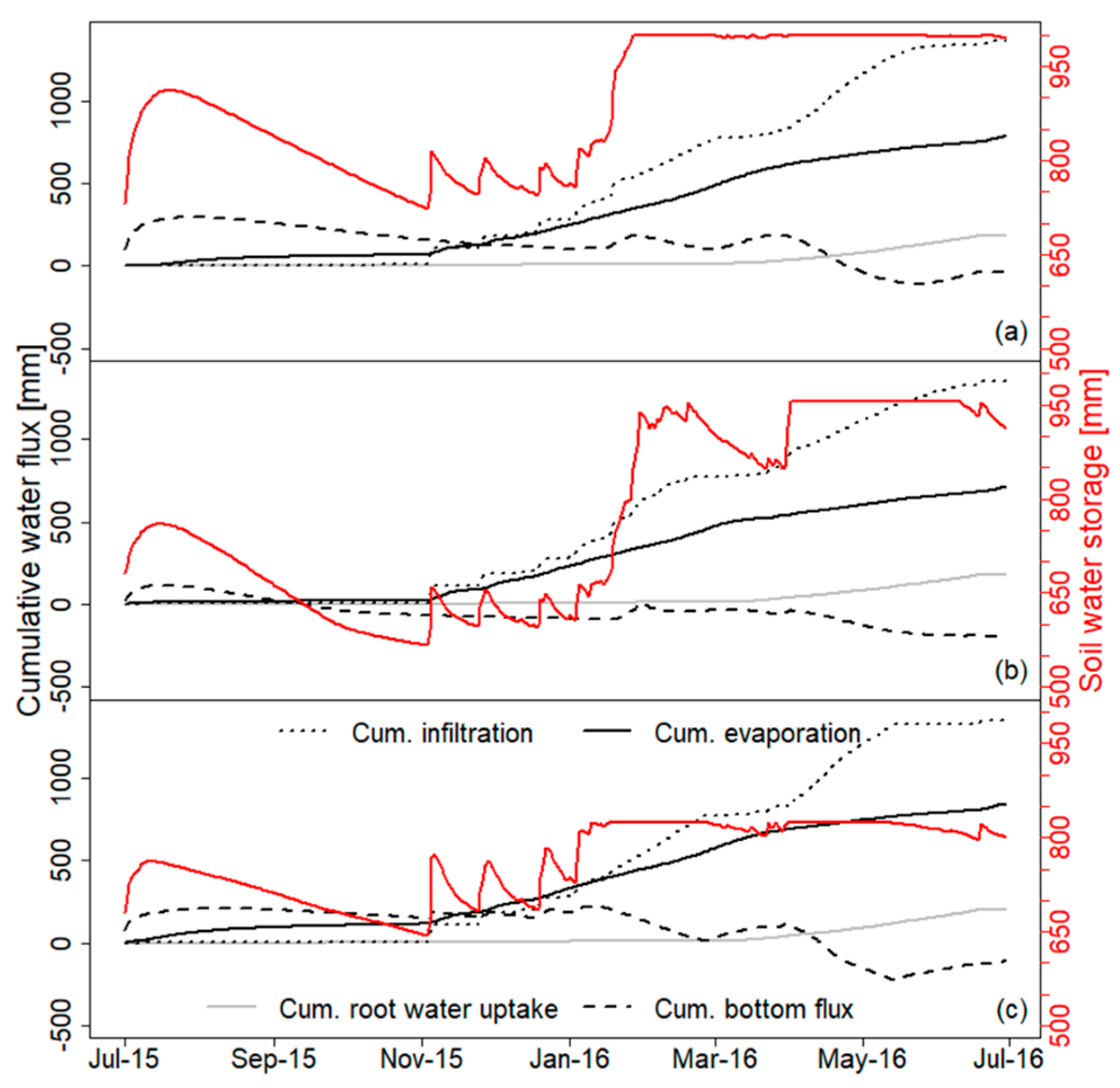
3.2. Soil Water Availability at the Different Hydrological Zones

To assess soil water availability, annual soil water balance was established at each hydrological zone for a period of one year (July 2015 to June 2016). Modeled water fluxes showed high temporal variability (Figure 8) and distinct differences in annual values (

Table 11. Annual water balance from the Hydrus-1D method for each hydrological zone.

Hydrological Zone	P	ETp	ETa	Go	Gi	ΔS
			mm
Riparian zone	1364.7	1561.0	969.4	108.9	296.2	262.8
Middle	1364.7	1561.0	896.1	196.4	116.2	232.9
Fringe	1364.7	1561.0	1043.9	219.8	222.2	120.1

P, precipitation; ET_p, potential evapotranspiration; ET_a, actual evapotranspiration; G_o, groundwater recharge; G_i, capillary rise/groundwater discharge; ΔS, change in soil water storage.

) among the three hydrological zones. Results showed positive and negative cumulative bottom flux among the three hydrological zones for the simulation period. Negative bottom flux indicated drainage from the profile and groundwater recharge. Moreover, positive bottom fluxes were associated with capillary rise and groundwater discharge. The highest positive cumulative bottom flux was observed at the riparian zone (296.2 mm), and the lowest value was observed at the middle zone (116.2 mm) of the floodplain during the simulation period (Figure 8).

The largest annual change in soil water storage was observed at the riparian zone. An increase of about 262.8 mm was calculated at the riparian zone, followed by the middle zone (232.9 mm), and fringe zone (120.1 mm) (Table 11). During the short (October to December 2015) and long (March to June 2016) rainy seasons, as well as the months of January and February 2016, soil water storage increased due to the filling up of the soil profile by the infiltration process. While in the dry season (July to September 2015), soil water storage gradually decreased at all of the hydrological zones. It should be noted that, at the middle zone, the decrease reached values below zero (Figure 8).

Cumulative root water uptake was highest at the fringe zone, followed by the middle and riparian zones (Figure 8). Annual cumulative root water uptake reached 201.0 mm at the fringe, 183.3 mm at the middle, and 183.5 mm at the riparian zones. Annual cumulative evaporation was substantially higher at the fringe (842.9 mm) than the riparian (785.9 mm) and middle (712.8 mm) zones during the simulation period. Therefore, actual evapotranspiration was highest at the fringe zone (1043.9 mm), contributing to 76.5% of the water loss from precipitation, followed by the riparian zone (969.4 mm, 71% water loss), and the middle zone (896.1 mm, 65.7% water loss) at each hydrological zone (Table 11).

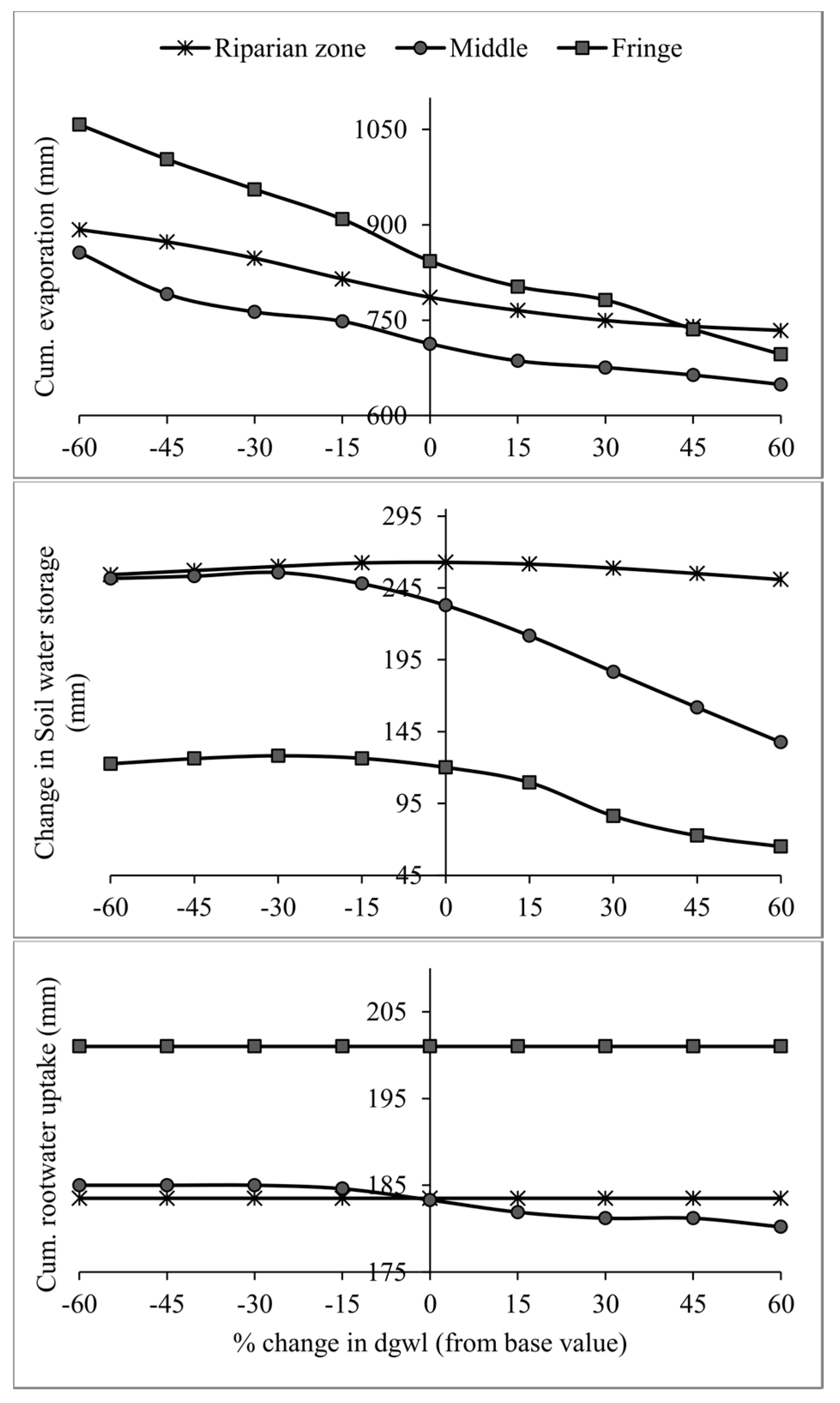
3.3. Sensitivity Analysis

Sensitivity analysis was performed to analyze the impact of changes in the depth to groundwater level on root water uptake, evaporation, and change in soil water storage. Figure 9 and

Table 12. Sensitivity indices (SI) for different water fluxes calculated after changes in the dgwl.

Water Flux Component	SI-15% dgwl	SI-30% dgwl	SI-45% dgwl	SI-60% dgwl
Riparian zone
cum. evaporation	0.063	0.125	0.169	0.202
Change in soil water storage	0.003	0.005	0.008	0.013
Cum. root water uptake	0.000	0.000	0.000	0.000
Middle zone
Cum. evaporation	0.087	0.122	0.139	0.291
Change in soil water storage	0.156	0.297	0.392	0.489
Cum. root water uptake	0.015	0.021	0.021	0.026
Fringe zone
Cum. evaporation	0.126	0.206	0.317	0.429
Change in soil water storage	0.140	0.349	0.446	0.480
Cum. root water uptake	0.000	0.000	0.000	0.000

Numbers in bold are the most sensitive parameters at each hydrological zone.

show the results of the sensitivity analysis. The sensitivity analysis revealed that among the water flux components, evaporation was the most sensitive parameter to changes in the dgwl, followed by change in soil water storage at all of the hydrological zones (Table 12 and Figure 9). Root water uptake was sensitive at the middle zone, while it was insensitive to changes in the dgwl at the fringe and riparian zones (Figure 9 and Table 12). Change in soil water storage and evaporation were highly sensitive at the fringe followed by the middle zone. The most sensitive parameter at the fringe and middle zones was change in soil water storage, while evaporation was highly sensitive at the fringe zone for all of the changes in the dgwl. Sensitivity indices increased with increase in changes to the dgwl for all of the water flux components at the three hydrological zones (Table 12).

At the fringe zone, cumulative evaporation and change in soil water storage had the maximum annual values of 1057.7 mm and 128.2 mm, higher than their respective references when the dgwl decreased by 60% and 30%, respectively. The minimum values of 696.4 mm and 65.0 mm for cumulative evaporation and change in soil water storage, respectively, were observed when the dgwl increased by 60% from the reference (Figure 9). In summary, the sensitivity analysis results indicate that very shallow or very deep groundwater levels will have great impacts on evaporation and change in soil water storage.

4. Discussion

The variations between calibrated and measured saturated hydraulic conductivity can be partly explained by the existence of macro pores [83,84] due to soil cracking, as well as by the sampling and measurement errors [85]. The discrepancies between measured and modeled soil moisture content are probably indicative of soil heterogeneity, model uncertainty, and measurement errors, which are inevitable in field conditions and the model setup [34,86]. Overall, the calibrated soil water model Hydrus-1D simulated the spatial soil moisture dynamics at the different hydrological zones in a reasonable manner. Therefore, the model can be used to predict spatial soil moisture dynamics as well as to close soil moisture data gaps within sites of similar biophysical properties, and rainfall in the floodplain. The results also demonstrate that Hydrus-1D is an effective tool for evaluating soil water dynamics [31,32,35,87,88] and hence would be acceptable for performing scenario simulations. The findings of the current study corroborate with those of Reference [33], who successfully applied a calibrated Hydrus-1D model with soil moisture measurements from one site to predict soil moisture conditions at another site, given that the biophysical properties and rainfall were similar. The results of Reference [89] further confirm the ability of the Hydrus model to reproduce spatial soil moisture content dynamics in floodplains, although the study applied the Hydrus-2D version.

Our observations and modeling results showed a distinct spatial pattern of the soil moisture time series along the defined hydrological zones. Soil moisture content increased from the surface layer (10-cm depth) to the bottom layer (40-cm depth). Furthermore, soil moisture content and change in soil water storage increased towards the riparian zone. Since all of the hydrological zones have similar rainfall levels, land use, and are situated a few kilometers apart from each other, the dynamics in soil moisture content and change in soil water storage can be explained by the depth to groundwater level according to the distance from the river, overbank flow, atmospheric influence, and soil properties.

Factors such as flooding from river overbank flow, rainfall, and seasonally shallow depth to groundwater level replenish soil water storage and soil moisture content at the riparian and middle zones during the long rainy season. Conversely, the fringe zone does not experience flooding from river overbank flow due to the distance from the river. Rainfall and lateral flow from the mountains are the main sources of water causing flooding [49] and replenishment of the soil water storage at the fringe zone. During the dry and short rainy seasons, soil moisture dynamics at the riparian and middle zones is mainly controlled by atmospheric influence, rainfall, soil properties, and the influence of the river water level on the depth to groundwater. Furthermore, the riparian and middle zones are directly connected to the river [49]. Therefore, a decrease or increase in the river water level directly impacts the depth to groundwater level in these zones. Similar results on the direct impact of the river water level on the depth to groundwater level in floodplains have been observed by References [90,91,92,93]. Soil moisture dynamics in the dry and short rainy seasons is independent of the influence from the depth to groundwater level at the riparian and middle zones of the floodplain, as indicated by both the modeled and measured time series. Similar results from Reference [43] indicated that decreasing low flows were directly linked to the surface water-groundwater interaction in the floodplain during the dry season, altering the depth to groundwater level dynamics and hence the soil water availability in the floodplain of Kilombero valley. The soil water storage after flood recession at the riparian and middle zones provides conditions for the cultivation of short-cycled upland crops like vegetables following the lowland rice; however, at the fringe zone, the soil water storage and the low depth to groundwater level throughout the year provides an opportunity for the cultivation of deep-rooted upland crops.

Furthermore, the increasing clay and soil organic carbon content towards the riparian zone could partly explain the high soil water storage observed at this zone. Our results show high soil moisture content with increasing clay content in soils, which is in line with studies by References [33,94]. From the theoretical point of view, the observed increasing soil organic carbon and clay content towards the riparian zone would imply high residual and saturated water content [95,96]. Subsequently, the riparian zone of the floodplain has a high agricultural production potential.

Atmospheric influence, especially of the potential evapotranspiration on soil moisture dynamics, is more pronounced at the fringe zone. The highest actual evapotranspiration at the fringe zone could partly explain the lowest soil moisture content observed at this zone. Actual evapotranspiration is always lower than the potential evapotranspiration at all of the hydrological zones, thus indicating limited water availability [97,98]. The high sensitivity of actual evaporation and soil water storage to changes in the depth to groundwater level was indicative of the influence of the groundwater table. Comparing the different hydrological zones, the highest sensitivity of actual evaporation at the fringe zone could be partly explained by the relatively low depth to groundwater level observed during the study throughout the year, as a result of direct recharge and lateral flow from the surrounding mountains [49]. For this reason, to reduce the loss of soil water through evaporation, soil and water management strategies like mulching can be used for sustainable agricultural production at the local scale.

The temporal soil moisture variability at the fringe zone is mainly determined by the depth to the groundwater (more so during the dry and short rainy seasons, during which soil moisture was directly responsive to changes in the depth to groundwater), soil properties, precipitation, and atmospheric influence. Similar findings were observed by Reference [99], who conducted a study in the alluvial floodplain of the Baratz Lake watershed, in the northwest of Sardinia, Italy. Their study showed that groundwater dynamics in the floodplain are an important source of temporal variability in soil moisture and vertical recharge processes in the alluvial floodplain. On the contrary, at the riparian and middle zones, soil moisture content is less responsive to the depth to groundwater level, which continuously declines as soil moisture directly responds to rain events during the short rainy season. This finding is supported by the sensitivity analysis results, which showed that variations in the depth to groundwater level have a greater impact on soil water storage at the fringe than at middle and riparian zones of the floodplain. Therefore, agricultural practices that might cause the depth to groundwater level to decline further have to be implemented with caution, especially at the fringe zones, whose soil moisture dynamics, soil water storage, and evapotranspiration are strongly controlled by the groundwater level. Our sensitivity analysis results indicate that an increase in the depth to groundwater level below the surface will decrease soil water storage and actual evapotranspiration at all of the hydrological zones.

The observed high positive cumulative bottom flux at riparian and fringe zones compared to the middle zone could be due to the contribution of groundwater flow from overbank flow towards the riparian zones and lateral flow from the mountains to the fringes. For a detailed understanding of the interacting hydrological processes among the river, floodplain, and its headwaters, the current Hydrus-1D model has to be extended to a 2D model. This will explicitly account for the lateral flows and subsurface runoff, which are not taken into account by the current model used in this study. Nonetheless, the model is adequate as the first attempt in the Kilombero floodplain to achieve the study objectives.

5. Conclusions

The Hydrus-1D model was calibrated and validated using daily field measurements of soil moisture content, over a period of one year in the floodplain of the Kilombero catchment, southern Tanzania. Simulated soil moisture content from the model fit quite well with the measured values at all of the four soil depths for all of the hydrological zones. Calibrated soil water model at one site can be used to predict spatial soil moisture content, as well as to close data gaps at other sites within the hydrological zone, with similar biophysical properties and rainfall levels.

Soil water storage increases towards the riparian zone. The highest evapotranspiration is observed at the fringe, followed by the riparian and middle zones. The riparian zone has the highest capillary rise and groundwater discharge, followed by the fringe and middle zones. The fringe zone maintains a relatively low depth to groundwater level throughout the year due to the lateral flow contribution from mountains.

Flooding from river overbank flow, local rainfall, and groundwater contribution replenish soil water storage during the long rainy season at the riparian and middle zones. A combination of local rainfall and lateral flow from mountains are the main sources of water supply at the fringe zone, replenishing soil water storage during the long rainy season. During the dry season, soil properties and atmospheric influence control change in soil water storage and soil moisture dynamics at the riparian and middle zones, whereas, in addition to these factors, the depth to groundwater and lateral flow from mountains play an important role in controlling soil moisture dynamics at the fringe zone. In the short rainy seasons, local rainfall and soil properties control soil moisture dynamics at the riparian and middle zones. Local rainfall, soil properties, lateral flow from mountains, and depth to groundwater level control soil moisture dynamics at the fringe zone.

Actual evaporation and change in soil water storage are highly sensitive to changes in the depth to groundwater level at all of the hydrological zones. It is worth noting that the sensitivity of actual evaporation and change in soil water storage is highest at the fringe zone.

The results help gain a better understanding of the groundwater-soil water interactions, and may provide references for wetland conservation and sustainable agricultural water management. The calibrated and validated model can be used for climate and land use scenario studies. This study has shown that local-scale water fluxes and soil moisture availability are driven by catchment-scale processes. Flooding of the riparian zone depends on catchment-scale processes, which are sensitive to land use and climate change [43]. Lateral fluxes and groundwater availability at the fringe will be influenced by land use and climate change. However, the one of the limitations of the study was it inability to describe the lateral flow; henceforth, in analyzing future water availability, the 1D modeling approach used in this study has to be linked to a 3D catchment-scale model that is able to provide the lower boundary conditions required to run Hydrus-1D as well as account for the lateral flows within the floodplain.

References

1. Blume, T.; Zehe, E.; Bronstert, A. Use of soil moisture dynamics and patterns at different spatio-temporal scales for the investigation of subsurface flow processes. Hydrol. Earth Syst. Sci. 2009, 13, 1215–1233. [Google Scholar] [CrossRef]
2. Venkatesh, B.; Lakshman, N.; Purandara, B.K.; Reddy, V.B. Analysis of observed soil moisture patterns under different land covers in Western Ghats, India. J. Hydrol. 2011, 397, 281–294. [Google Scholar] [CrossRef]
3. Qiu, Y.; Fu, B.; Wang, J.; Chen, L. Soil moisture variation in relation to topography and land use in a hillslope catchment of the Loess Plateau, China. J. Hydrol. 2001, 240, 243–263. [Google Scholar] [CrossRef]
4. Schenk, H.J.; Jackson, R.B. Rooting depths, lateral root spreads and below-ground / above-ground allometries of plants in water-limited. J. Ecol. 2002, 90, 480–494. [Google Scholar] [CrossRef]
5. Mulebeke, R.; Kironchi, G.; Tenywa, M.M. Soil moisture dynamics under different tillage practices in cassava—Sorghum based cropping systems in eastern Uganda. Ecohydrol. Hydrobiol. 2013, 13, 22–30. [Google Scholar] [CrossRef]
6. Böhme, B.; Becker, M.; Diekkrüger, B.; Förch, G. How is water availability related to the land use and morphology of an inland valley wetland in Kenya? Phys. Chem. Earth 2016, 93, 84–95. [Google Scholar] [CrossRef]
7. Wu, D.D.; Anagnostou, E.N.; Wang, G.; Moges, S.; Zampieri, M. Improving the surface-ground water interactions in the Community Land Model: Case study in the Blue Nile Basin. Water Resour. Res. 2014, 50, 8015–8033. [Google Scholar] [CrossRef]
8. Sánchez, N.; Martínez-fernández, J.; González-piqueras, J.; González-dugo, M.P. Agricultural and Forest Meteorology Water balance at plot scale for soil moisture estimation using vegetation parameters. Agric. For. Meteorol. 2012, 166–167, 1–9. [Google Scholar] [CrossRef]
9. Vereecken, H.; Huisman, J.A.; Bogena, H.; Vanderborght, J.; Vrugt, J.A.; Hopmans, J.W. On the value of soil moisture measurements in vadose zone hydrology: A review. Water Resour. Res. 2008, 44, 1–21. [Google Scholar] [CrossRef]
10. Zehe, E.; Graeff, T.; Morgner, M.; Bauer, A.; Bronstert, A. Plot and field scale soil moisture dynamics and subsurface wetness control on runoff generation in a headwater in the Ore Mountains. Hydrol. Earth Syst. Sci. 2010, 14, 873–889. [Google Scholar] [CrossRef] [Green Version]
11. Mitsch, W.; Gosselink, J.G. Wetlands of the World; John Wiley and Sons, Inc.: Hoboken, NJ, USA, 2015; ISBN 978-1-119-01979-4. [Google Scholar]
12. McCartney, M.; Rebelo, L.-M.; Senaratna Sellamuttu, S.; De Silva, S. Wetlands, Agriculture and Poverty Reduction; IWMI Research Report; International Water Management Institue: Colombo, Sri Lanka, 2010; Volume 137, ISBN 9290907347. Available online: http://citeseerx.ist.psu.edu/viewdoc/download?doi=10.1.1.188.4594&rep=rep1&type=pdf (accessed on 5 November 2017).
13. Thompson, J.R.; Polet, G. Hydrology and land use in a sahelian floodplain wetland 1. Wetlands 2000, 20, 639–659. [Google Scholar] [CrossRef]
14. Von Der Heyden, C.J.; New, M.G. The role of a dambo in the hydrology of a catchment and the river network downstream. Hydrol. Earth Syst. Sci. 2003, 7, 339–357. [Google Scholar] [CrossRef]
15. Acreman, M.C.; Miller, F. Hydrological impact assessment of wetlands. Int. Symp. Groundw. Sustain. 2007, 225–255. Available online: http://aguas.igme.es/igme/isgwas/Ponencias%20ISGWAS/16-Acreman.pdf (accessed on 10 February 2018).
16. Dixon, A.B.; Wood, A.P. Wetland cultivation and hydrological management in eastern Africa: Matching community and hydrological needs through sustainable wetland use. Nat. Resour. Forum 2003, 27, 117–129. [Google Scholar] [CrossRef]
17. Wood, A.; van Halsema, G.E. Scoping Agriculture—Wetland Interactions; FAO: Rome, Italy, 2008; ISBN 9789251060599. [Google Scholar]
18. Reddy, K.R.; DeLaune, R.; Craft, C.B. Nutrients in Wetlands: Implications to Water Quality under Changing Climatic Conditions. 2010. Available online: https://thewaternetwork.com/_/hydrogeology-and-groundwater-remediation/document-XAs/nutrients-in-wetlands-implications-to-water-quality-under-changing-climatic-conditions-dcI85SV8e8QkZG4d8mRIYg (accessed on 9 February 2018).
19. Sakané, N.; Alvarez, M.; Becker, M.; Böhme, B.; Handa, C.; Kamiri, H.W.; Langensiepen, M.; Menz, G.; Misana, S.; Mogha, N.G.; et al. Classification, characterisation, and use of small wetlands in East Africa. Wetlands 2011, 31, 1103–1116. [Google Scholar] [CrossRef]
20. Futoshi, K. Development of a major rice cultivation area in the Kilombero valley, TANZANIA. Afr. Study Monogr. Suppl. 2007, 36, 3–18. [Google Scholar]
21. Nindi, S.J.; Maliti, H.; Kija, H.; Machoke, M. Conflicts over land and water resources in the kilombero valley floodplain, Tanzania. African Study Monogr. Suppl. 2014, 50, 173–190. [Google Scholar]
22. Paul, H.; Steinbrecher, R. New Alliance for Food Security and Nutrition. Who Benefits, Who Loses? Technical Report; Econexus: Oxford, UK, 2013; Available online: http://www.econexus.info/sites/econexus/files/African_Agricultural_Growth_Corridors_&_New_Alliance_-_EcoNexus_June_2013.pdf (accessed on 10 November 2017).
23. Rosenbaum, U.; Bogena, H.R.; Herbst, M.; Huisman, J.A.; Peterson, T.J.; Weuthen, A.; Western, A.W.; Vereecken, H. Seasonal and event dynamics of spatial soil moisture patterns at the small catchment scale. Water Resour. Res. 2012, 48, 1–22. [Google Scholar] [CrossRef]
24. Mohanty, B.P.; Cosh, M.H.; Lakshmi, V.; Montzka, C. Soil Moisture Remote Sensing: State-of-the-Science. Vadose Zone J. 2017, 16. [Google Scholar] [CrossRef]
25. RoTimi Ojo, E.; Bullock, P.R.; Fitzmaurice, J. Field Performance of Five Soil Moisture Instruments in Heavy Clay Soils. Soil Sci. Soc. Am. J. 2015, 79, 20–29. [Google Scholar] [CrossRef]
26. Singh, R.; Singh, J. Irrigation planning in cotton through simulation modeling. Irrig. Sci. 1996, 17, 31–36. [Google Scholar] [CrossRef]
27. Šimůnek, J.; Šejna, M.; Saito, H.; Sakai, M.; van Genuchten, M.T. The HYDRUS-1D Software Package for Simulating the One-Dimensional Movement of Water, Heat, and Multiple Solutes in Variably-Saturated Media; Manual Version 4.17; Univeristy of California: Riverside, CA, USA, 2013; Available online: https://www.pc-progress.com/en/Default.aspx?hydrus-1d (accessed on 20 May 2016).
28. Varut, G.; Wei, X.; Huang, D.; Shinde, D.; Price, R. Application of MODHMS to Simulate Integrated Water Flow and Phosphorous Transport in a Highly Interactive Surface Water Groundwater System along the Eastern Boundary of the Everglades National Park, Florida. In Proceedings of the MODFLOW and More 2011: Integrated Hydrologic Modeling the Colorado School of Mines, Golden, CO, USA, 5–8 June 2011. [Google Scholar]
29. Graham, D.N.; Butts, M.B. Flexible, integrated watershed modelling with MIKE SHE. In Watershed Models; Singh, V.P., Frevert, D.K., Eds.; CRC Press: Boca Raton, FL, USA, 2005; pp. 245–272. ISBN 0849336090. [Google Scholar]
30. Šimůnek, J.; van Genuchten, M.T.; Šejna, M. Hydrus: Model use, calibration, and validation. Trans. ASABE 2012, 55, 1261–1274. [Google Scholar]
31. Kandelous, M.M.; Kamai, T.; Vrugt, J.A.; Šimunek, J.; Hansona, B.; Hopmans, J.W. Evaluation of subsurface drip irrigation design and management parameters for alfalfa. Agric. Water Manag. 2012, 109, 81–93. [Google Scholar] [CrossRef]
32. Siyal, A.A.; Bristow, K.L.; Šimůnek, J. Minimizing nitrogen leaching from furrow irrigation through novel fertilizer placement and soil surface management strategies. Agric. Water Manag. 2012, 115, 242–251. [Google Scholar] [CrossRef]
33. Chen, M.; Willgoose, G.R.; Saco, P.M. Spatial prediction of temporal soil moisture dynamics using HYDRUS-1D. Hydrol. Process 2014, 28, 171–185. [Google Scholar] [CrossRef]
34. Jing, L.; Zhang, Z.; Ni, L. Evaluation of water movement and water losses in a direct-seeded-rice field experiment using Hydrus-1D. Agric. Water Manag. 2014, 142, 38–46. [Google Scholar] [CrossRef]
35. Li, H.; Yi, J.; Zhang, J.; Zhao, Y.; Si, B.; Hill, R.L.; Cui, L.; Liu, X. Modeling of soil water and salt dynamics and its effects on root water uptake in Heihe arid wetland, gansu, China. Water 2015, 7, 2382–2401. [Google Scholar] [CrossRef]
36. Xu, X.; Zhang, Q.; Li, Y.; Li, X. Evaluating the influence of water table depth on transpiration of two vegetation communities in a lake floodplain wetland. Hydrol. Res. 2016, 47, 293–312. [Google Scholar] [CrossRef]
37. Böhme, B.; Becker, M.; Diekkrüger, B. Calibrating FDR sensor for soil moisture monitoring in a wetland in Central Kenya. Phys. Chem. Earth 2013, 66, 101–111. [Google Scholar] [CrossRef]
38. Gabiri, G.; Diekkrüger, B.; Leemhuis, C.; Burghof, S.; Näschen, K.; Asiimwe, I.; Bamutaze, Y. Determining hydrological regimes in an agriculturally used tropical inland valley wetland in Central Uganda using soil moisture, groundwater, and digital elevation data. Hydrol. Process. 2018, 32, 349–362. [Google Scholar] [CrossRef]
39. Snyder, G.H. Everglades agricultural area soil subsidence and land use projections. Soil Crop Sci. Soc. Fla. Proc. 2005, 64, 44–51. [Google Scholar]
40. Sławiński, C.; Cymerman, J.; Witkowska-Walczak, B.; Lamorski, K. Impact of diverse tillage on soil moisture dynamics. Int. Agrophys. 2012, 26, 301–309. [Google Scholar] [CrossRef]
41. Mombo, F.; Speelman, S.; Van Huylenbroeck, G.; Hella, J.; Moe, S. Ratification of the Ramsar convention and sustainable wetlands management: Situation analysis of the Kilombero Valley wetlands in Tanzania. J. Agric. Ext. Rural Dev. 2011, 3, 153–164. [Google Scholar]
42. Mwalyosi, R.B.B. Resource Potentials of Tanzania Basin, the Rufiji River. Ambio 2000, 19, 16–20. [Google Scholar]
43. Leemhuis, C.; Thonfeld, F.; Näschen, K.; Steinbach, S.; Muro, J.; Strauch, A.; Ander, L.; Daconto, G.; Games, I. Sustainability in the Food-Water-Ecosystem Nexus: The Role of Land Use and Land Cover Change for Water Resources and Ecosystems in the Kilombero Wetland, Tanzania. Sustainability 2017, 9, 1513. [Google Scholar] [CrossRef]
44. Koutsouris, A.J.; Chen, D.; Lyon, S.W. Comparing global precipitation data sets in eastern Africa: A case study of Kilombero Valley, Tanzania. Int. J. Climatol. 2016, 36, 2000–2014. [Google Scholar] [CrossRef]
45. Beck, A.D. The Kilombero valley of south-central Tanganyika. East Afr. Geogr. Rev. 1964, 1964, 37–43. [Google Scholar]
46. Bonarius, H. Physical Properties of Soils in the Kilombero Valley (Tanzania); German Agency for Technical Cooperation, Ltd. (GTZ): Stuttgarter, Germany, 1975; Available online: https://library.wur.nl/isric/fulltext/isricu_i2757_001.pdf (accessed on 30 June 2016).
47. Department of the Interior, U.S.G.S. Product Guide—Landsat 4–7 Surface Reflectance (LEDAPS) Product Version 8.0. Available online: https://landsat.usgs.gov/sites/default/files/documents/ledaps_product_guide.pdf (accessed on 6 August 2017).
48. Department of the Interior, U.S.G.S. Product Guide Landsat 8 Surface Reflectance Code (LASRC) Product Version 4.1. Available online: https://landsat.usgs.gov/sites/default/files/documents/lasrc_product guide.pdf (accessed on 6 August 2017).
49. Burghof, S.; Gabiri, G.; Stumpp, C.; Chesnaux, R.; Reichert, B. Development of a hydrogeological conceptual wetland model in the data-scarce north-eastern region of Kilombero. Hydrogeol. J. 2017. [Google Scholar] [CrossRef]
50. Daniel, S.; Gabiri, G.; Kirimi, F.; Glasner, B.; Näschen, K.; Leemhuis, C.; Steinbach, S.; Mtei, K. Spatial distribution of soil hydrological properties in the Kilombero floodplain, Tanzania. Hydrology 2017, 4, 57. [Google Scholar] [CrossRef]
51. Stevens Water Monitoring Systems, Inc. The Hydra Probe® Soil Sensor Users Manual; Stevens Water Monitoring Systems, Inc.: Portland, OR, USA, 2007; pp. 1–63. [Google Scholar]
52. Delta-T Devices Ltd. User Manual for the Profile Probe Type PR2; Delta-T Devices Ltd.: Burwell, Cambridge, UK, 2006; Volume 104, Available online: https://www.delta-t.co.uk/product/pr2/ (accessed on 15 March 2014).
53. Decagon Devices Inc. 5TE Manuals; Decagon Devices Inc.: Pullman, WA, USA, 2016; Available online: http://manuals.decagon.com/Manuals/13509_5TE_Web.pdf (accessed on 15 April 2016).
54. Evett, S.R.; Tolk, J.A.; Howell, T.A. Soil profile water content determination: Sensor accuracy, axial response, calibration, temperature dependence, and precision. Vadose Zone J. 2006, 5, 894–907. [Google Scholar] [CrossRef]
55. Evett, S.R.; Schwartz, R.C.; Tolk, J.A.; Howell, T.A. Soil profile water content determination: Spatiotemporal variability of electromagnetic and neutron probe sensors in access tubes. Vadose Zone J. 2009, 8, 926–941. [Google Scholar] [CrossRef]
56. Delta-T Devices Ltd. User Manual for the Moisture Meter Type HH2; Delta-T Devices Ltd.: Cambridge, UK, 2013; Volume 124. [Google Scholar] [CrossRef]
57. Sensor Transmitter Systems GmBH Datalogger DL/N 70; Software and Accessories. STS Sensors Transmitter Systems GmbH: Sindelfingen, Germany, 2012. Available online: https://www.stssensoren.de/datenlogger/ (accessed on 20 April 2014).
58. Horiba Scientific. A Guidebook to Particle Size Analysis; Horiba Instruments, INC.: Irvine, CA, USA, 2010; Available online: www.horiba.com/us/particle (accessed on 15 July 2015).
59. Okalebo, J.R.; Gathua, K.W.; Woomer, P.L. Laboratory Methods of Soil and Plant Analysis: A Working Manual, 2nd ed.; Sacred African Publishers: Nairobi, Kenya, 2002; Available online: http://www.kalro.org:8080/repository/bitstream/0/8547/1/lab methods of soil and plant analysis.pdf (accessed on 17 August 2016).
60. Eijkelkamp Laboratory. Permeameters: User Manual, Soil and Water. 2013, pp. 1–14. Available online: https://en.eijkelkamp.com/products/laboratory-equipment/soil-water-permeameters.html (accessed on 10 March 2014).
61. Radcliffe, D.; Šimůnek, J. Soil Physics with HYDRUS: Modeling and Applications; CRC Press, Taylor & Francis Group: Boca Raton, FL, USA, 2010. [Google Scholar]
62. Van Genuchten, M.T. A closed-form Equation for predicting Hydraulic Conductivity of Unsaturated soils. Soil Sci. Soc. Am. J. 1980, 44, 892–898. [Google Scholar] [CrossRef]
63. Soylu, M.E.; Istanbulluoglu, E.; Lenters, J.D.; Wang, T. Quantifying the impact of groundwater depth on evapotranspiration in a semi-arid grassland region. Hydrol. Earth Syst. Sci. 2011, 15, 787–806. [Google Scholar] [CrossRef] [Green Version]
64. Allen, R.G.; Pereira, L.S.; Raes, D.; Smith, M.; Ab, W. Crop Evapotranspiration—Guidelines for Computing Crop Water Requirements—FAO Irrigation and Drainage Paper 56; FAO: Rome, Italy, 1998; pp. 1–15. [Google Scholar]
65. Senay, G.B.; Leake, S.; Nagler, P.L.; Artan, G.; Dickinson, J.; Cordova, T.; Glenn, E.P. Estimating basin scale evapotranspiration (ET) by water balance and remoting sensing methods. Hydrol. Process. 2011, 25, 4037–4049. [Google Scholar] [CrossRef]
66. Flint, A.L.; Childs, S.W. Use of the Priestley-Taylor evaporation equation for soil water limited conditions in a small forest clearcut. Agric. For. Meteorol. 1991, 56, 247–260. [Google Scholar] [CrossRef]
67. Peacock, C.E.; Hess, T.M. Estimating evapotranspiration from a reed bed using the Bowen ratio energy balance method. Hydrol. Process. 2004, 18, 247–260. [Google Scholar] [CrossRef]
68. Jensen, D.T.; Hargreaves, G.H.; Temesgen, B.; Allen, R.G. Computation of ETo under Nonideal Conditions. J. Irrig. Drain. Eng. 1997, 123, 394–400. [Google Scholar] [CrossRef]
69. Danner, M.; Locherer, M.; Hank, T.; Richter, K. Measuring Leaf Area Index (LAI) with the LI-Cor LAI 2200C or LAI-2200 (+2200Clear Kit)—Theory, Measurement, Problems, Interpretation; EnMAP Field Guide Technical Report; GFZ Data Services: Postam, Germany, 2015. [Google Scholar] [CrossRef]
70. Schaap, M.G.; Leij, F.J.; Genuchten, M.T. Van rosetta: A computer program for estimating soil hydraulic parameters with hierarchical pedotransfer functions. J. Hydrol. 2001, 251, 163–176. [Google Scholar] [CrossRef]
71. Singh, R.; Van Dam, J.C.; Feddes, R.A. Water productivity analysis of irrigated crops in Sirsa district, India. Agric. Water Manag. 2006, 82, 253–278. [Google Scholar] [CrossRef]
72. Slaton, N.A.; Beyrouty, C.A.; Wells, B.R.I.; Norman, R.J.; Gbur, E.E. Root growth and distribution of two short-season rice genotypes. Plant Soil 1990, 121, 269–278. [Google Scholar] [CrossRef]
73. Gupta, H.V.; Kling, H.; Yilmaz, K.K.; Martinez, G.F. Decomposition of the mean squared error and NSE performance criteria: Implications for improving hydrological modelling. J. Hydrol. 2009, 377, 80–91. [Google Scholar] [CrossRef]
74. Gupta, H.V.; Sorooshian, S.; Yapo, P.O. Status of automatic calibration for hydrologic models: Comparison with multilevel expert calibration. J. Hydrol. Eng. 1999, 4, 135–143. [Google Scholar] [CrossRef]
75. Moriasi, D.N.; Arnold, J.G.; Van Liew, M.W.; Binger, R.L.; Harmel, R.D.; Veith, T.L. Model evaluation guidelines for systematic quantification of accuracy in watershed simulations. Trans. ASABE 2007, 50, 885–900. [Google Scholar] [CrossRef]
76. Nash, J.E.; Sutcliffe, J.V. River flow forecasting through conceptual models part I—A discussion of principles. J. Hydrol. 1970, 10, 282–290. [Google Scholar] [CrossRef]
77. Bidlake, W.R. Evapotranspiration from a bulrush dominated wetland in the Klamath Basin, Oregon. J. Am. Water Resour. Assoc. 2000, 36, 1309–1320. [Google Scholar] [CrossRef]
78. Giertz, S.; Diekkrüger, B.; Steup, G. Physically-based modelling of hydrological processes in a tropical headwater catchment (West Africa)—Process representation and multi-criteria validation. Hydrol. Earth Syst. Sci. 2006, 10, 829–847. [Google Scholar] [CrossRef]
79. Pianosi, F.; Beven, K.; Freer, J.; Hall, J.W.; Rougier, J.; Stephenson, D.B.; Wagener, T. Sensitivity analysis of environmental models: A systematic review with practical workflow. Environ. Model. Softw. 2016, 79, 214–232. [Google Scholar] [CrossRef] [Green Version]
80. Hastenrath, S.; Nicklis, A.; Greischar, L. Atmospheric-hydrospheric mechanisms of climate anomalies in the western equatorial Indian Ocean. J. Geophys. Res. 1993, 98, 20219–20235. [Google Scholar] [CrossRef]
81. Goddard, L.; Graham, N.E. Importance of the Indian Ocean for simulating rainfall anomalies over eastern and southern Africa. J. Geophys. Res. 1999, 104, 19099–19116. [Google Scholar] [CrossRef]
82. Black, E.; Slingo, J.M.; Sperber, K.R. An observational study of the relationship between excessively strong short rains in coastal East Africa and Indian Ocean SST. Mon. Weather Rev. 2003, 74–94. [Google Scholar] [CrossRef]
83. Guber, A.; Tuller, M.; San, F.; Martinez, J.; Iassonov, P.; Martin, M.A. The through Porosity of Soils as the Control of Hydraulic Conductivity. In Proceedings of the 19th World Congress of Soil Science, Soil Solutions for a Changing World, Brisbane, Australia, 1–6 August 2010; pp. 80–83. [Google Scholar]
84. Bodner, G.; Scholl, P.; Loiskandl, W.; Kaul, H. Geoderma Environmental and management influences on temporal variability of near saturated soil hydraulic properties. Geoderma 2013, 204–205, 120–129. [Google Scholar] [CrossRef] [PubMed]
85. Ritter, A.; Hupet, F.; Muñoz-Carpena, R.; Lambot, S.; Vanclooster, M. Using inverse methods for estimating soil hydraulic properties from field data as an alternative to direct methods. Agric. Water Manag. 2003, 59, 77–96. [Google Scholar] [CrossRef]
86. Gribb, M.M.; Forkutsa, I.; Hansen, A.; David, G.; Chandler, J.P.M. The Effect of Various Soil Hydraulic Property Estimates on Soil Moisture Simulations. Vadose Zone J. 2009, 8, 321–331. [Google Scholar] [CrossRef]
87. Li, Y.; Šimunek, J.; Wang, S.; Yuan, J.; Zhang, W. Modeling of soil water regime and water balance in a Transplanted Rice Field Experiment with Reduced Irrigation. Water 2017, 9, 248. [Google Scholar] [CrossRef]
88. Schwärzel, K.; Šimunek, J.; van Genuchten, M.Th.; Wessolek, G. Measurement and modeling of soil-water dynamics and evapotranspiration of drained peatland soils. J. Plant Nutr. Soil Sci. 2006, 169, 762–774. [Google Scholar] [CrossRef]
89. Joris, I.; Feyen, J. Modelling water flow and seasonal soil moisture dynamics in analluvial groundwater-fed wetland. Hydrol. Earth Syst. Sci. 2003, 7, 57–66. [Google Scholar] [CrossRef]
90. Alden, A. Assessment of River floodplain Aquifer interaction. Environ. Eng. Geosci. 1997, 3, 537–548. [Google Scholar] [CrossRef]
91. Sophocleous, M. Interactions between groundwater and surface water: The state of the science. Hydrogeol. J. 2002, 10, 52–67. [Google Scholar] [CrossRef]
92. Doble, R.C.; Crosbie, R.S.; Smerdon, B.D.; Peeters, L.; Cook, F.J. Groundwater recharge from overbank floods. Water Resour. Res. 2012, 48, 1–14. [Google Scholar] [CrossRef]
93. Karim, F.; Kinsey-Henderson, A.; Wallace, J.; Godfrey, P.; Arthington, A.H.; Pearson, R.G. Modelling hydrological connectivity of tropical floodplain wetlands via a combined natural and artificial stream network. Hydrol. Process. 2013. [Google Scholar] [CrossRef]
94. Markewitz, D.; Devine, S.; Davidson, E.A.; Brando, P.; Nepstad, D.C. Soil moisture depletion under simulated drought in the Amazon: Impacts on deep root uptake. New Phytol. 2010, 187, 592–607. [Google Scholar] [CrossRef] [PubMed]
95. Amundson, R. The carbon budget in soils. Annu. Rev. Earth Planet. Sci. 2001, 29, 535–562. [Google Scholar] [CrossRef]
96. Rawls, W.J.; Pachepsky, Y.A.; Ritchie, J.C. Effect of soil organic carbon on soil water retention. Geoderma 2003, 116, 61–76. [Google Scholar] [CrossRef]
97. Verstraeten, W.W.; Veroustraete, F.; Feyen, J. Assessment of Evapotranspiration and Soil Moisture Content Across Different Scales of Observation. Sensors 2008, 8, 70–117. [Google Scholar] [CrossRef] [PubMed]
98. Lu, N.; Chen, S.; Wilske, B.; Sun, G.; Chen, J. Evapotranspiration and soil water relationships in a range of disturbed and undisturbed ecosystems in thethe semi-arid Inner Mongolia, China. J. Plant Ecol. 2017, 4, 49–60. [Google Scholar] [CrossRef]
99. Pirastru, M.; Niedda, M. Evaluation of the soil water balance in an alluvial flood plain with a shallow groundwater table. Hydrol. Sci. J. 2013, 58, 898–911. [Google Scholar] [CrossRef]
Figure 1. (a) Location of study area andoverview of hydrological zones and instrumentation; and (b) detailed instrumentation at each hydrological zone used for modeling.
Water 10 00191 g001
Figure 2. Daily rainfall and ET0 values used during the simulation period.
Water 10 00191 g002
Figure 3. Measured and modeled soil moisture content for calibration at the four plots in the riparian zone. (a,b) plot PR_4; (c,d) plot PR_1; (e,f) plot PR_8; (g,h) plot PR_3. dgwl, measured depth to groundwater level.
Water 10 00191 g003
Figure 4. Measured and modeled soil moisture content after calibration at the four plots for the middle zone. (a,b) plot PM_3; (c,d) plot PM_5; (e,f) plot PM_7. dgwl; measured depth to groundwater level.
Water 10 00191 g004
Figure 5. Measured and modeled soil moisture content after calibration at the four plots for the fringe zone. (a,b) plot PF_12; (c,d) plot PF_10; (e,f) plot PF_4; (g,h) plot PF_8. dgwl; measured depth to groundwater level.
Water 10 00191 g005
Figure 6. Comparison of measured (averaged from all plots) and modeled soil moisture from the averaged calibrated hydraulic parameters at each hydrological zone. (ac) Riparian zone; (df) middle zone; (gi) fringe zone. dgwl: measured depth to groundwater level.
Water 10 00191 g006
Figure 7. Modeled and measured soil moisture content from selected plots at depths of 10 and 30 cm in each hydrological zone. PR, PM, PF represent riparian, middle, and fringe zones, respectively. (a,b) Riparian; (c,d) middle; and (e,f) fringe zones. 1, 3, 4, 5, 7, 8, 10, and 12 denote plot numbers at the different hydrological zones.
Water 10 00191 g007
Figure 8. Cumulative (Cum.) water fluxes for one year. (a) Riparian zone; (b) middle zone; and (c) fringe zone.
Water 10 00191 g008
Figure 9. Sensitivity analysis for different water fluxes on changes in the depth to groundwater level; dgwl, depth to groundwater level.
Water 10 00191 g009