Abstract
Runoff in snowy alpine regions is sensitive to climate change in the context of global warming. Exploring the impact of climate change on the runoff in these regions is critical to understand the dynamics of the water cycle and for the improvement of water resources management. In this study, we analyzed the long-term variations in annual runoff in the headwaters region of the Yellow River (HRYR) (a typical snowy mountain region) during the period of 1956–2012. The Soil and Water Assessment Tool (SWAT) with different elevation bands was employed to assess the performance of monthly runoff simulations, and then to evaluate the impacts of climate change on runoff. The results show that the observed runoff for the hydrological stations at lower relative elevations (i.e., Maqu and Tangnaihai stations) had a downward trend, with rates of 1.91 and 1.55 mm/10 years, while a slight upward trend with a rate of 0.26 mm/10 years was observed for the hydrological station at higher elevation (i.e., Huangheyan station). We also found that the inclusion of five elevation bands could lead to more accurate runoff estimates as compared to simulation without elevation bands at monthly time steps. In addition, the dominant cause of the runoff decline across the whole HRYR was precipitation (which explained 64.2% of the decrease), rather than temperature (25.93%).
1. Introduction
The hydrological cycle is one of the most important natural biospheric processes. It provides humans, animals, and plants with water. It also moves materials such as nutrients, pathogens, and sediment into and out of aquatic ecosystems. Global climate change is very likely to affect the hydrological cycle, and consequently, water resources by increasing evaporation due to rising temperatures and by changing precipitation patterns [1]. Over the past century, the climate has changed dramatically at the global scale, with the average global surface temperature having increased by approximately 0.8 °C [2]. Global warming and its variability are expected to intensify the global hydrological cycle, which could transform the timing and magnitude of runoff, resulting in increased frequency and intensity of extreme events such as flood and drought [3]. This may occur especially in cold highland regions [4], as temperatures strongly modulate snow accumulation and melt, thus affecting the hydrological systems originating from these regions. These changes, in turn, are expected to affect water supply systems, sediment transport and deposition, food production, power generation, and ecosystem conservation [5]. Highland regions in the headwaters of large rivers provide a large fraction of the life-sustaining water resources for the entire globe [3]. Changes in their water yield will affect the ecology and economy of the middle and lower reaches of these basins. Therefore, it is essential to investigate and quantify the hydrological response to the climate change of highland regions at the basin scale. Research at this scale is useful not only for developing a deeper understanding of watershed hydrological cycles, but also for providing better information applicable to the sustainable development of water resources and the maintenance of stable ecosystems.
Hydrological models are widely used to evaluate and quantify the effects of climate change on water resources [6,7]. Of these, the Soil and Water Assessment Tool (SWAT) has been most widely used across the world [8,9,10,11], because it is a distributed hydrological model that can reflect the spatial distribution characteristics of the terrain, soil, vegetation, land use, and precipitation. In addition, because the SWAT model treats sub-basins as independent units with similar hydrological characteristics, SWAT produces more reasonable hydrological calculations and is convenient for comprehensive planning and management of watersheds. Moreover, sub-basins in the model are generated based on digital elevation model (DEM) data, and their size can be adjusted by setting the critical source area of the sub-basin within the SWAT model as needed, which makes the SWAT model more flexible. Furthermore, the SWAT model has proved to be suitable in northwest China (which is where the study region is located), despite the sparse observational information (e.g., precipitation stations and temperature stations). The success of the model in these conditions is due to the inclusion of a weather generator within the SWAT model, which can automatically generate meteorological driver data based on long-term observed meteorological data that are available. Most importantly, the SWAT model has been successfully employed to assess the impacts of climate change on surface runoff variation in the headwater region of the Yellow River (HRYR) in previous studies. Therefore, the SWAT model was our top choice to employ in this study. In addition, it has also proven to be an effective tool for simulating hydrological processes, soil erosion, and contaminant transport under different environmental conditions all over the world [8,9]. Zhang, et al. [11] employed the SWAT model to assess the impacts of climate change and human activities on runoff changes in the Huifa River basin in China from 1965 to 2005. Their research indicated that the impacts of climate change could result in a decrease in runoff, accounting for −36.7, −59.5, +36.9, and −45.2 mm/a for 1965–1975, 1976–1985, 1986–1995, and 1996–2005, respectively. Githui, et al. [12] assessed the climate change impact on SWAT-simulated runoff in western Kenya, and their results showed that changes in the annual mean rainfall of 2.4% to 23.2% corresponded to changes in runoff between approximately 6% and 115%. Khoi used the SWAT model to evaluate the effects of climate change on streamflow in the Srepok watershed in Vietnam. The results showed that a 1.3 to 3.9 °C increase in annual temperature and a 0.5% to 4.4% decrease in annual precipitation could correspond to a decrease in streamflow of about 2.8% to 7.6%. Yin, et al. [13] used the SWAT model to identify the effects of climate changes and land use/land cover changes on runoff in a semi-humid to semi-arid transition zone in northwest China. Their work suggested that land use/land cover change was the major cause of runoff reduction, contributing to 44% of the runoff variation between the 1980s and 1990s, and 71% of the runoff variation between the 1990s and 2000s.
For alpine regions, elevation is an important factor in determining changes in many meteorological variables, including temperature and precipitation [14,15]. SWAT users have the option to improve hydrological simulation performance over mountainous headwaters using elevation bands, which modulate the amount of precipitation input depending on the orography of the catchment [14,15]. The SWAT elevation bands are established by specifying the number of bands, their average elevation [8], and the proportion of the sub-basin area they each contain. To account for the topographic effects of climate variables, SWAT allows up to ten elevation bands to be declared in each sub-basin, allowing the user to simulate snow and snowmelt separately for each elevation zone [16].
Previous researchers have investigated the effects of elevation bands on hydrological simulations. Zhang, et al. [14] assessed the benefits for runoff simulations of modeling snow with and without elevation bands, and the results showed that the performance of simulations using elevation bands is much more accurate than that of simulations without elevation bands. When Zhang, et al. [15] evaluated the performance of SWAT-based runoff simulations in the northeast of the Tibetan Plateau, they found that the SWAT model performed better for both calibration and validation periods after establishing elevation bands, as compared to applying the model without using elevation bands. When Pradhanang, et al. [17] employed SWAT to compare snowpack and snowmelt simulated with different numbers of elevation bands (i.e., one, three, and five elevation bands) for the Cannonsville reservoir watershed in the northeastern United States, their results indicated that the simulations for both daily and seasonal streamflow could be improved to achieve satisfactory performance (i.e., a coefficient of determination of 0.73 and a Nash–Sutcliffe coefficient of 0.72) when using three elevation bands. However, although most previous researchers have reported that incorporating elevation bands could improve the performance of hydrological simulations, few studies have addressed finding the optimal number of elevation bands that should be used in runoff simulations across alpine regions.
The HRYR, located in the eastern region of the Tibetan Plateau, is widely known as the “water tower” of the Yellow River, as it accounts for only 15% of the entire Yellow River basin area but contributes approximately 38% of the total flow [18]. In recent years, the HRYR has been suffering critical eco-environmental problems, including declining groundwater levels, shrinking of lakes and wetlands, thawing of glaciers and permafrost, degradation of vegetation health, and decreasing runoff [19]. Such changes in hydrological conditions could have an important impact not only on the local environment and socio-economic development but also on conditions in downstream areas. Therefore, it is critical that we accurately simulate hydrological processes and, in particular, the response of runoff to climate change in this region.
Previous studies have tried to determine the reasons for decreased runoff within the HRYR, and many have suggested that climate change has been the primary cause of the decrease in runoff [20,21]. However, most of these studies have applied statistical approaches (e.g., Budyko and double accumulative curve methods), and the results could not capture physical processes well due to the lack of physical mechanisms in these approaches. Furthermore, since few efforts have systematically evaluated the effects of snowmelt on surface runoff or have established appropriate elevation bands for hydrological simulation in this heterogeneous alpine region, there is still no consensus on the recommended number of elevation bands for alpine hydrological simulation [14,17]. More importantly, all existing studies have only identified generalized impacts of climate change on runoff variation, and the individual impacts of precipitation and temperature on runoff variation are still unclear. Therefore, to better understand how the effects of climate change contribute to runoff variation, a SWAT-based quantitative assessment is needed.
The main objectives of this study are (1) to explore the changes in the observed annual runoff across the HRYR; (2) to evaluate the effect of the elevation band method on SWAT-based monthly runoff simulations in the HRYR; and (3) to further quantify the impacts of climate change on runoff variation.
2. Study Area and Data Sources
The headwater region of the Yellow River (HRYR; 32°5′ N–36°30′ N, 95°30′ E–103°30′ E) lies in the basin above the Tangnaihai hydrological station of the Yellow River in the eastern Qinghai-Tibet Plateau region (Figure 1). The drainage area of the HRYR is about 121,972 km2 (15% of the whole Yellow River basin), while contributing approximately 40% of the total flow in the Yellow River basin. Therefore, the HRYR is often called the “water tower” of the Yellow River. The average annual temperature is 0.26 °C, ranging from a minimum annual average temperature of −5.38 °C to a maximum of 4.14 °C. The average annual precipitation is 534 mm, ranging from a minimum annual average precipitation of 262 mm to a maximum of 772 mm. The altitude in most areas ranges from 2568 to 6264 meters, with an average of 4,217 meters. The mainland cover in this study area is alpine meadows and grasslands, which covers almost 80% of the whole region [21], with lakes and swamps covering an area of about 2000 km2.
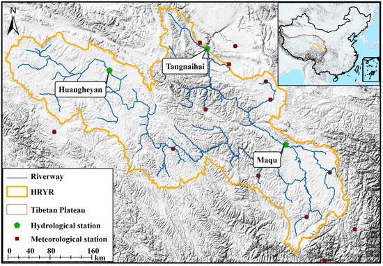
Figure 1.
The location map of the headwater region of the Yellow River (HRYR) and selected hydroclimatic stations.
Monthly average runoff data (1964–2012) from the three hydrological gauging stations selected to calibrate the model (i.e., Huangheyan, Tangnaihai, and Maqu (Figure 1) were obtained from the Yellow River Conservancy Commission. Meteorological data including the daily maximum temperatures, daily minimum temperatures, relative humidity, hours of sunshine, and wind speed from the period 1964 to 2012 were obtained from the China Meteorological Data Sharing Service System (http://www.escience.gov.cn). Data from 15 meteorological stations were used in the model. Most of the stations were situated near the Tangnaihai and Maqu hydrological stations. DEM data and land-use information were obtained from the Resources and Environmental Science Data Center of the Chinese Academy of Sciences (http://www.resdc.cn). Soil data consisting of soil type maps (1:1,000,000) and records of related soil properties were obtained from the Cold and Arid Region Science Data Center of the Chinese Academy of Sciences (http://westdc.westgis.ac.cn). Of these observational datasets, the meteorological data, DEM data, land-use data, and soil data were used as the inputs to drive the SWAT model, and the observed runoff data were used to calibrate and validate the SWAT model.
3. Methodology
3.1. The Mann-Kendall Test for Abrupt Change Analysis
The Mann-Kendall (M-K) test has been widely used for trend analysis of time series and testing for mutation points [22]. It can be used to determine if there are abrupt changes in a data series and indicate the start time and region of the abrupt changes. Compared to other abrupt change methods (e.g., Pettitt, Buishand range test, the standard normal homogeneity test), this test has the advantage of not assuming any distribution form for the data and has similar power to its parametric competitors [23]. In addition, the method has a high degree of quantification and is more suitable for rank variables [23]. Therefore, it is highly recommended for general use by the World Meteorological Organization and is widely used in the literature to analyze the abrupt change in meteorological and hydrological data [24,25]. For a time series (x1, x2, …, xn), the null hypothesis is stated as follows: the sample under investigation shows no beginning of a developing trend. The following test is performed to prove or to disprove the assumption, and for this, first the M-K test statistic is calculated as below:
for all j, where = 1 if > (j = 1, 2, …, i), and otherwise = 0. Assuming that the sequence is random and independent, the Sk is distributed as a normal distribution with the expected value of and the variance calculated as follows:
The statistical sequence can then be acquired as follows:
Zk is characterized by a normal distribution. Unlike the M-K test for the monotonic trend, which calculates the statistical variables only once for the entire sample, in the M-K test for abrupt change analysis, for the reverse sequence, the so-called retrograde is obtained similarly (xn, xn−1, xn−2, …, x1). The statistical variables , , and of the reverse sequence are calculated according to the same procedure as shown in Equations (1)–(4), respectively. The Z values calculated using the progressive and retrograde series are designated here as Z1 and Z2. If the intersection of the Z1 and Z2 curves is between the lines based on the 95% confidence interval (with a significance level of 0.05), it indicates that an abrupt change has taken place at that intersection point [26].
3.2. The Soil and Water Assessment Tool (SWAT) Model
3.2.1. Basic Introduction to SWAT
SWAT is a comprehensive, time-continuous, semi-distributed, process-based model developed by the US Department of Agriculture [27]. It is an effective tool for simulating various river flows over long periods of time. SWAT has been successfully applied in many parts of the world and has proven to be able to simulate hydrological processes, erosion, vegetation growth, and water quality changes [15,28] in large river basins, and it is useful for assessing the impacts of climate change and water management [29]. The first step in using this model is to divide the basin into sub-basins based on topography. SWAT subsequently determines the hydrological response units (HRUs) within each sub-basin based on soil, land use, and slope. The calculations for the hydrological cycle are based on water balance, which includes four storage volumes: snow, soil, shallow aquifers, and deep aquifers [30]. Using daily meteorological time series data as inputs, daily, monthly, and annual fluxes of water and solutes can be simulated in river basins at the HRU level and aggregated at the sub-basin level. Then, the loads are transported and routed toward the river and basin exits. The SWAT model has been selected for this study because it has been successfully applied to various scales, topographies, and climatic conditions around the globe. In addition, SWAT can successfully simulate streams in high mountains when an improved snow melting algorithm is implemented [16]. More information about this model can be obtained from the official model literature [31].
3.2.2. Snowmelt Processes in the SWAT Model
Snowmelt is primarily controlled by the temperature of air and snow, the rate of the melting, and the areal coverage of the snow. The SWAT model uses a temperature-index-based method to estimate the snowmelt process. The model considers snowmelt as rainfall to calculate runoff and seepage. In calculating the snowmelt, the rainfall energy from the snow melting portion is set to zero, and the peak runoff rate is estimated assuming snow melted uniformly over the 24 hours of the day [32]. Temperature is considered to be the main controlling factor for snow melting in the temperature index method. The snowmelt is estimated as a linear function of the difference between the average of snowpack temperature and maximum air temperature on a given day and the base, or threshold temperature, for the snowmelt [33],
where is the amount of snowmelt on a given day (mm H2O), is the melt factor for the day (mm H2O/[day∙°C]), is the fraction of the HRU area covered by snow, Tsnow is the snowpack temperature on a given day (°C), and Tmx is the maximum air temperature for a given day (°C). Tmlt is the base temperature above which snowmelt is allowed (°C). The melt factor allows for seasonal variations, with maximum and minimum values occurring in summer and winter, respectively, and is calculated as:
where and are the melt factors for June 21st (mm H2O/[day∙°C]) and 21 December (mm H2O/[day∙°C]), respectively, and is the day number of the year.
3.2.3. Elevation Bands in the SWAT Model
Elevation is an important factor in determining changes in many meteorological variables, including temperature and precipitation [14,15]. To account for the topographic effects of climate variables, SWAT allows up to ten elevation bands to be defined in each sub-basin to simulate snow and snowmelt separately for each elevation zone [16]. SWAT can better represent the precipitation and temperature distribution of areas containing large elevation variations by the addition of these elevation bands. Precipitation and temperature for each band are calculated as a function of the respective lapse rate and the difference between the gauge elevation and the average elevation specified for the band [16]. The temperature and precipitation of each band were adjusted using the following two equations:
where is the elevation band mean temperature (°C), T is the temperature measured at the weather station (°C), is the mean elevation in the elevation band (m), EL is the elevation of the weather station (m), is the mean precipitation in the elevation band (mm), P is the precipitation measured at the weather station (mm), is the precipitation lapse rate (mm/km), and is the temperature lapse rate (°C/km).
3.3. SWAT Model Setup
3.3.1. Model Sensitivity Analysis and Calibration
To take into consideration the continuity of meteorological and hydrological data, the model was calibrated with the observed monthly runoff dataset for the years 1966–1980 using 1964–1965 as a training period, based on the measured emissions records of the Tangnaihai and Maqu stations. The calibration period at the Huangheyan station was instead 1976–1980 due to the fact that there were missing data between 1964 and 1975. After calibration, the model was then validated using the 1981–1991 dataset. The sensitivity analysis and calibration were performed using SWAT calibration and uncertainty programs (SWAT-CUP [28,34]) with the Sequential Uncertainty Fitting algorithm version 2 (SUFI-2) [35]. The sensitivity analysis methodology was performed by the one-at-a-time procedure presented by [35]. This procedure tests the model sensitivity by changing one parameter at a time while all other parameters are kept constant. In the model, 33 parameters (Table 1) were considered in all, including 24 parameters for the hydrological component, 7 parameters for the snow component, and 2 parameters for the elevation bands analyses. The best values obtained for the 23 most sensitive parameters identified by SWAT-CUP for the three hydrological stations are listed in Table 2. After determining the most sensitive parameters, 1500 simulations [36] were performed for each iteration. The ranges of the parameters were modified after each iteration according to the new parameter ranges suggested by the procedure, taking into account reasonable physical limitations. More detailed information about the procedure for calibration of the model can be found in [35] and [37].

Table 1.
Basic information for parameters considered in the Soil and Water Assessment Tool (SWAT) model.
Table 2.
Best parameter range for the selected 23 most sensitive parameters in SWAT model hydrological simulations. Parameters beginning with “v__” and “r__” indicate a replacement and a relative change to the initial parameter values, respectively.
3.3.2. Model Performance Evaluation
In this study, the Nash–Sutcliffe coefficient (NS) and the coefficient of determination (R2) have been used as indicators for the best-fit simulations. The values of NS [38] and R2 [39] are calculated as
where represents the observed data; represents the model-simulated value; and are the mean of observed and model-simulated values for the entire time period of the evaluation, respectively; and i = 1, 2, …, N, where N is the total number of observed and simulated data pairs. NS measures the difference between the observed value and the simulated value. The value of NS closest to +1 indicates the best model performance. The value of NS can be divided into four levels [40]: very good performance (0.75 < NS ≤ 1), good performance (0.65 < NS ≤ 0.75), satisfactory performance (0.50 < NS ≤ 0.65), and unsatisfactory performance (NS ≤ 0.50). The value of R2 ranges from 0 to 1, indicating the level of similarity between the observed and simulated data. The higher the R2 value, the better the performance of the model.
3.4. Quantifying the Effects of Climate Variables on Runoff Variation
Hydrological models have become an increasingly important tool for quantifying the drivers of runoff change. We applied SWAT to evaluate the relative effects of temperature and precipitation on the variations observed in regional water resources. Based on the results of the abrupt change analysis, the time series for runoff were divided into two subperiods: One referred to as the baseline period (pre-change period) and the other as the variation period (post-change period). Because there were few inhabitants around the HRYR, we assumed the impacts of human activities on runoff changes could be neglected. Thus, the model was supposed to run without taking into account any effects of human influence on the study area. Therefore, the difference in simulated runoff before and after the abrupt change point can be attributed to climate change alone, and it can be expressed as:
where and indicate the annual mean simulated runoff for the variation period and the baseline period, respectively. Subsequently, the contributions of temperature and precipitation to runoff variations in the HRYR between 1992 and 2012 can be calculated as:
We left all inputs except precipitation and model setup unchanged and used the precipitation in the variation period to drive the model. Thus, the difference in runoff simulation between the variation period and the baseline period was denoted as . Similarly, the values and are the percentages of the precipitation and temperature contributions toward runoff changes, respectively.
4. Results and Discussion
4.1. Temporal Pattern of Long-Term Observed Variables
Figure 2a–c shows the temporal trends in the annual runoff during the period 1956–2012 based on the linear regression method (in green) and a 5-year moving average (in blue). It can be seen that, for the three hydrological series, the runoff series at Maqu and Tangnaihai stations had a downward trend, with rates of 1.91 mm/10 years (Figure 2b) and 1.55 mm/10 years (Figure 2c), respectively. By contrast, a slight upward trend with a rate of 0.26 mm/10 years (Figure 2a) was observed for the Huangheyan station. At the interdecadal scale, across all three stations, the runoff was relatively abundant in the 1960s and 1980s, while relatively less runoff occurred in the 1950s, 1990s, and 2000s. Annual average runoff depths were 33.5, 165.5, and 164.8 mm at Huangheyan, Maqu, and Tangnaihai stations, respectively. It can be clearly seen that the annual runoff at the Maqu and Tangnaihai stations located in the eastern HRYR was much greater than annual runoff at the Huangheyan station, located in the western HRYR.
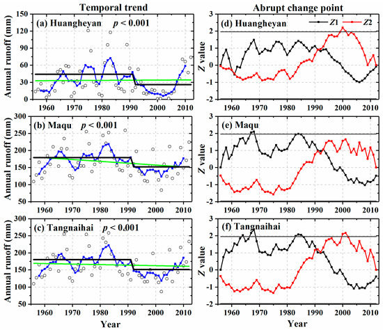
Figure 2.
Temporal trends (a–c) and abrupt change points (d–f) based on the Mann-Kendall (M-K) abrupt change test for the annual runoff time series during the period of 1956–2012 for the Huangheyan, Maqu, and Tangnaihai stations, located at points across the HRYR. The white circles show annual runoff values (in a–c), the green and blue lines (in a–c) show the long-term linear tendency and the 5-year moving average for the annual runoff, respectively. The black line (in a–c) shows the long-term average runoff for the periods before and after the year identified by the M-K abrupt change test. Z1 and Z2 (in d–f) are confidence lines at a significance level of p = 0.05. The abrupt change point according to the M-K test lies at the intersection between these lines.
The M-K abrupt change test was used to study change-point characteristics of runoff at these three stations. As shown in Figure 2d–f, the abrupt changes in runoff across all three stations were significant and the change years were all between 1991 and 1993. Although there was a slight difference in the timing of abrupt change of runoff among the three stations, we selected the year 1991 as the abrupt change year for consistency across the basin. We therefore further divided each series of runoff data into two periods: the baseline period (1971–1991) and the variation period (1992–2012). The multiyear average runoff was 44 mm/yr (for the baseline period) and 26 mm/yr (for the variation period) at Huangheyan; 179 mm/yr (baseline period) and 152 mm/yr (variation period) at Maqu; and 180 mm/yr (baseline period) and 151 mm/yr (variation period) at Tangnaihai. The multiyear average runoff was significantly smaller in the variation period than in the baseline period.
We further evaluated long-term temporal variations of meteorological variables, as shown in Figure S1. We observe that there are no significant variations in annual precipitation after the year 1991 (the change-point year based on the M-K abrupt change test) (Figure S1a), whereas for temperature, there are straightforward M-K variations for annual mean, minimum, and maximum temperatures (Figure S1b–d). As compared with our previous research [41], the frequency of occurrence of daily precipitation of more than 10 mm showed an upward trend. At the same time, the amount of precipitation did not change greatly, which means that the occurrence of dry days also showed an upward trend. With the temperatures increasing in alpine regions, this means the evapotranspiration could increase and the frozen soil layer could melt, especially with the minimum temperature increasing.
4.2. Evaluation of Effects of Elevation Bands on Monthly Runoff Simulation
Figure 3 shows the model performance without taking elevation bands into account for the three stations during the period of 1966–1992. We can see that the R2 values were roughly the same for the calibration and validation periods, especially for the Maqu and Tangnaihai stations (R2 > 0.8), while the NS values in the three sub-basins were almost all less than 0.5. This was especially notable for the Huangheyan station (NS = −0.31 in the calibration period), where this result was mainly because the simulated peak runoff was underestimated. In addition, there was an overall bias for the Huangheyan station, which may be because few meteorological stations were situated around Huangheyan station. The underestimation of the peak runoff is most likely due to the high heterogeneity in precipitation patterns and intensity caused by the high variability in the morphology and orography of these alpine basins [42]. In brief, without consideration of model uncertainties, the monthly runoff simulations without inclusion of elevation bands were found to be unsatisfactory (NS < 0.5) [40].
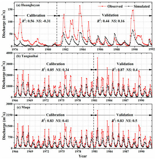
Figure 3.
Monthly runoff simulations compared to observations for the calibration period (1976–1980 for Huangheyan; 1966–1980 for Tangnaihai and Maqu) and the validation period (1981–1991) without the inclusion of elevation bands.
Figure 4 shows the evaluation coefficients for simulations using different numbers of elevation bands in the calibration period (1966–1980). Across the HRYR, the NS values for simulations with between one and ten elevation bands are all greater than the NS values for simulations without elevation bands in the calibration period. The same results were found for the validation period (Table 3). It also can be seen from Figure 4 that the R2 and NS values were highest for simulations using five elevation bands compared to simulations using other numbers of elevation bands. This means the inclusion of five elevation bands within the simulation can provide more accurate runoff estimates at monthly time steps for the HRYR.
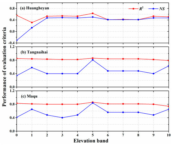
Figure 4.
Performance of evaluation criteria (coefficient of determination (R2) and Nash–Sutcliffe coefficient (NS) values) for simulations with different numbers of elevation bands during the calibration period (1976–1980 for Huangheyan; 1966–1980 for Tangnaihai and Maqu).
Table 3.
Model performance evaluation of monthly runoff using different numbers of elevation bands during the calibration period for three gauging stations. Values in parentheses represent statistics for the validation period (1981–1991). Statistics reported are the coefficient of variation (R2) and the Nash-Sutcliffe coefficient (NS).
The results from monthly runoff simulations with five elevation bands during the period of 1966–1992 are shown in Figure 5. In general, the magnitude and variation of the simulated monthly runoff for all three stations were similar to the observations, and the simulations were more accurate compared with the simulations that did not include elevation bands (Figure 4 and Figure 5). Notably, the results for Huangheyan were not as good as the results for the other two stations. The poor runoff simulations for the Huangheyan station was mostly because there were few meteorological stations situated around Huangheyan station, the meteorological input generated by weather could lead to a disagreement with the observed runoff [43,44]. In addition, the parameter uncertainty also existed in this simulation, although we have tried our best to calibrate the model. These results have indicated that the inclusion of elevation bands in the SWAT model plays an important role in streamflow simulations in snowy, mountainous areas. The precipitation will encounter a variety of potential conditions over various elevations: It may fall as rain at lower altitudes or as new snow at higher altitudes. In general, snow melts at lower altitudes, while with recent global warming, snow has begun to melt at a faster rate [45]. Hydrological processes may be changed slightly at different elevations, so employment of elevation bands in the SWAT model could better describe the hydrological processes for various elevations in snowy mountains regions, and thus it could greatly improve model performance in the HRYR.
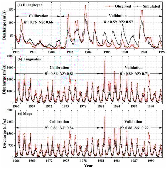
Figure 5.
Monthly runoff simulations compared to observations for the calibration period (1976–1980 for Huangheyan; 1966–1980 for Tangnaihai and Maqu) and the validation period (1981–1991) with five elevation bands.
4.3. Impact of Climate Change on Runoff in the HRYR
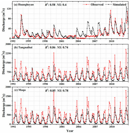
Figure 6 shows the simulated monthly runoff in the variation period (1992–2012) based on the calibrated parameters and inclusion of five elevation bands, alongside the corresponding observed runoff. The simulated runoff matched the observed runoff well overall for both peak and low flows at the three gauging stations, although the simulation was unsatisfactory for the Huangheyan station during the variation period (NS = 0.4; R2 = 0.58), which is reflected mainly in the overestimation of monthly runoff. The overestimation was most likely due to the fact that there are insufficient meteorological stations near the Huangheyan hydrological station, which therefore could not adequately reflect the actual climatic conditions. In addition, the relatively complex natural and geographic environment of this region could be increasing the difficulty of runoff simulation. For example, there were certain differences in the amount of solar radiation received on the various slope directions and slope areas in alpine regions, which could have led to the differences in temperature changes and further affected the distribution of snow cover, redistribution, and ablation [46]. Overall, the model is still applicable in the variation period, indicating that the underlying surface conditions in the HRYR have not changed much since 1992. The underlying surface conditions referred to the indicated land-use and reservoir changes, which were caused mainly by human activities. As shown in Figure 6, we could see that, except for at Huangheyan station, the simulated runoff of the other two stations was satisfactory when using the same model setup and model parameters as within the baseline period, which further testified that there were no significant impacts of human activities on runoff. Therefore, climate changes are the main reasons for runoff reduction during the variation period (1997–2011) in the HRYR, which is consistent with the findings of most previous studies [19,47,48]. This result is mostly because the HRYR is a cold, high-altitude region with few humans, there are no large dams or irrigation projects in this area, and there is only one small hydroelectric generating station, located downstream of Eling Lake, with a maximum storage capacity of 15.2 × 10⁸ m3 [49]. Therefore, going forward, this study area can be considered a relatively pristine region that has only lightly been affected by human activities.
Among the effects of climate change on runoff, temperature and precipitation are two important meteorological factors affecting hydrological processes [18]. Table 4 and Figure 7 show the relative contributions of precipitation and temperature to changes in the observed runoff between 1992 and 2012 in the HRYR. Runoff was more sensitive to precipitation variations at the Tangnaihai and Maqu stations, while it was more sensitive to temperature variations at the Huangheyan station. Because the average elevation of the area around the Huangheyan station is higher than the average elevation around the other two stations, the Huangheyan station region includes large areas of glaciers and frozen soil; therefore, increased temperatures around this station can exacerbate the degradation of permafrost and the melt of glacial snow cover [50], which can lead to significant changes in regional ecosystems and water cycles [51,52]. In addition to temperature and precipitation, other climate variables such as net radiation, wind speed, and relative humidity can also affect runoff changes. All of them could act on runoff by altering precipitation and temperature. If we consider Tangnaihai station, which is located at the outlet of the HRYR, as an indicator of the basin-scale dynamics, all in all, we can conclude that across the whole HRYR, precipitation played a dominant role in runoff change during the variation period (64.2%), although the impacts of temperature on runoff changes (25.93%) should certainly not be ignored.
Table 4.
Proportional influence of temperature and precipitation on decreases in runoff in the HRYR, estimated with the SWAT model for different stations.
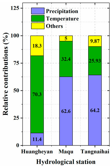
Figure 7.
Relative contributions of temperature, precipitation, and other climate variables to changes in observed runoff across the HRYR.
4.4. Limitations and Uncertainties
In order to better understand the long-term effects of precipitation and temperature on runoff changes of the HRYR, we have conducted here a quantitative analysis using the results of the SWAT hydrological model. Although these quantitative results are informative, some limitations and uncertainties still remain. First and foremost, our quantitative results were based on the assumption that precipitation and temperature are independent. However, in reality, these two factors are interrelated and they interact continuously [53,54]. Second, there are model structure uncertainties, which are mainly caused by the assumptions and simplifications of the model. For example, there are two channel-routing methods used within the SWAT model (the specific river length method and the Muskingum method); the use of a different method could lead to different output [55]. In this study, we employed the Muskingum method, which was the default equation and has been used in almost all previous studies [7,56,57] including in the HRYR [15]. Third, with respect to input data uncertainties, only 15 meteorological stations were available and used. Furthermore, these stations were situated nearer to Tangnaihai and Maqu, which could lead to simulation inaccuracy for Huangheyan station. However, a weather generator within the SWAT model was used to generate forcing data based on long-term, historical meteorological data. The model simulation result was satisfactory, despite remaining uncertainties in the model parameters. Lastly, the observed runoff data that were used to calibrate and validate the model actually were influenced to some extent by human activities. However, in order to calculate the impacts of climate change on runoff variations, we used the simulation results rather than the observed data, which in effect removed the impacts of human activities on runoff variation, as the inputs used for both the baseline period and the variation period were identical except for the meteorological data. All of these factors could be affecting the accuracy of the simulations at some level, although we have minimized the impacts.
5. Conclusions
In this study, we evaluated the performance of the Soil and Water Assessment Tool (SWAT) model in the HRYR, which is a cold, mountainous region with a complex natural and geographic environment. With well-adjusted calibration parameters, the model performance statistics improved for the HRYR when using the elevation band approach. We also found that the inclusion of five elevation bands led to a satisfactory monthly hydrological simulation. The inclusion of elevation bands within the model could lead to a better understanding of snow and glacier melting processes at different altitudes. Therefore, it is strongly recommended to apply the elevation band approach to cold mountain basins.
In addition, with the employment of the SWAT model in the HRYR, we validated the claim that the major factor to reduce runoff in this region has been climate change, with precipitation playing a dominant role in runoff change (64.2%), while finding also that the impacts of temperature on runoff changes (25.93%) should not be ignored. In addition, we found that runoff is more sensitive to temperature variations in the area around the Huangheyan station, mainly because it is located at high altitude and has large areas of glaciers and frozen soil; consequently, increasing temperatures could exacerbate the degradation of permafrost and the melt of glacial snow cover already happening in this region.
Although there are limitations and uncertainties of model performance at the monthly scale, the results obtained from this study can be used as a reference for regions with similarly complex terrain in order to obtain better modeling results using the SWAT model. Moreover, the results could deepen our understanding of mountain hydrological responses to climate change. This will eventually provide useful knowledge that will help local governments take efficient measures to mitigate the negative impacts of regional environmental changes on the survival and agricultural production of local herders and farmers.
Supplementary Materials
The following are available online at https://www.mdpi.com/2073-4433/10/9/509/s1, Figure S1: Long-term temporal trend of mean basin precipitation and temperature during 1960–2012 across the headwater region of yellow river.
Author Contributions
Data curation, J.W. and Y.X.; formal analysis, H.Z.; methodology, J.W., H.Z., and Y.X.; software, J.W. and Y.X.; supervision, J.W. and H.Z.; writing—original draft, J.W., H.Z., and Y.X.; writing—review and editing, J.W.
Funding
This research was funded by the National Natural Science Foundation of China (No. 41622101), the State Key Laboratory of Earth Surface Processes and Resource Ecology, and the Fundamental Research Funds for the Central Universities.
Acknowledgments
We are grateful to the Yellow River Conservancy Commission (YRCC) for providing the monthly runoff data (http://www.yellowriver.gov.cn/other/hhgb/) and the China Meteorological Administration (CMA) for providing the climate datasets (http://data.cma.cn/).
Conflicts of Interest
The authors declare no conflict of interest.
References
- Huntington, T.G. Evidence for intensification of the global water cycle: Review and synthesis. J. Hydrol. 2006, 319, 83–95. [Google Scholar] [CrossRef]
- Hansen, J.; Sato, M.; Ruedy, R.; Lo, K.; Lea, D.W.; Medina-Elizade, M. Global temperature change. Proc. Natl. Acad. Sci. USA 2006, 103, 14288–14293. [Google Scholar] [CrossRef] [PubMed]
- Beniston, M. Climatic change in mountain regions: A review of possible impacts. Clim. Change 2003, 59, 5–31. [Google Scholar] [CrossRef]
- Jiang, T.; Chen, Y.Q.D.; Xu, C.Y.Y.; Chen, X.H.; Chen, X.; Singh, V.P. Comparison of hydrological impacts of climate change simulated by six hydrological models in the Dongjiang Basin, South China. J. Hydrol. 2007, 336, 316–333. [Google Scholar] [CrossRef]
- Lin, Y.P.; Chen, C.J.; Lien, W.Y.; Chang, W.H.; Petway, J.R.; Chiang, L.C. Landscape Conservation Planning to Sustain Ecosystem Services under Climate Change. Sustainability 2019, 11, 1393. [Google Scholar] [CrossRef]
- Ahn, K.H.; Merwade, V. Quantifying the relative impact of climate and human activities on streamflow. J. Hydrol. 2014, 515, 257–266. [Google Scholar] [CrossRef]
- Wu, J.W.; Miao, C.Y.; Wang, Y.M.; Duan, Q.Y.; Zhang, X.M. Contribution analysis of the long-term changes in seasonal runoff on the Loess Plateau, China, using eight Budyko-based methods. J. Hydrol. 2017, 545, 263–275. [Google Scholar] [CrossRef]
- Grusson, Y.; Sun, X.L.; Gascoin, S.; Sauvage, S.; Raghavan, S.; Anctil, F.; Sachez-Perez, J.M. Assessing the capability of the SWAT model to simulate snow, snow melt and streamflow dynamics over an alpine watershed. J. Hydrol. 2015, 531, 574–588. [Google Scholar] [CrossRef]
- Yen, H.; Sharifi, A.; Kalin, L.; Mirhosseini, G.; Arnold, J.G. Assessment of model predictions and parameter transferability by alternative land use data on watershed modeling. J. Hydrol. 2015, 527, 458–470. [Google Scholar] [CrossRef]
- Malago, A.; Efstathiou, D.; Bouraoui, F.; Nikolaidis, N.P.; Franchini, M.; Bidoglio, G.; Kritsotakis, M. Regional scale hydrologic modeling of a karst-dominant geomorphology: The case study of the Island of Crete. J. Hydrol. 2016, 540, 64–81. [Google Scholar] [CrossRef]
- Zhang, A.J.; Zhang, C.; Fu, G.B.; Wang, B.D.; Bao, Z.X.; Zheng, H.X. Assessments of Impacts of Climate Change and Human Activities on Runoff with SWAT for the Huifa River Basin, Northeast China. Water Resour. Manag. 2012, 26, 2199–2217. [Google Scholar] [CrossRef]
- Githui, F.; Gitau, W.; Mutua, F.; Bauwens, W. Climate change impact on SWAT simulated streamflow in western Kenya. Int. J. Climatol. 2009, 29, 1823–1834. [Google Scholar] [CrossRef]
- Yin, J.; He, F.; Xiong, Y.J.; Qiu, G.Y. Effects of land use/land cover and climate changes on surface runoff in a semi-humid and semi-arid transition zone in northwest China. Hydrol. Earth Syst. Sci. 2017, 21, 183–196. [Google Scholar] [CrossRef]
- Zhang, X.S.; Srinivasan, R.; Debele, B.; Hao, F.H. Runoff simulation of the headwaters of the Yellow River using the SWAT model with three snowmelt algorithms. J. Am. Water Resour. Assoc. 2008, 44, 48–61. [Google Scholar] [CrossRef]
- Zhang, Y.G.; Su, F.G.; Hao, Z.C.; Xu, C.Y.; Yu, Z.B.; Wang, L.; Tong, K. Impact of projected climate change on the hydrology in the headwaters of the Yellow River basin. Hydrol. Process. 2015, 29, 4379–4397. [Google Scholar] [CrossRef]
- Fontaine, T.A.; Cruickshank, T.S.; Arnold, J.G.; Hotchkiss, R.H. Development of a snowfall-snowmelt routine for mountainous terrain for the soil water assessment tool (SWAT). J. Hydrol. 2002, 262, 209–223. [Google Scholar] [CrossRef]
- Pradhanang, S.M.; Anandhi, A.; Mukundan, R.; Zion, M.S.; Pierson, D.C.; Schneiderman, E.M.; Matonse, A.; Frei, A. Application of SWAT model to assess snowpack development and streamflow in the Cannonsville watershed, New York, USA. Hydrol. Process. 2011, 25, 3268–3277. [Google Scholar] [CrossRef]
- Li, L.; Ha, Z.C.; Wang, J.H.; Wang, Z.H.; Yu, Z.B. Impact of future climate change on runoff in the head region of the Yellow River. J. Hydrol. Eng. 2008, 13, 347–354. [Google Scholar] [CrossRef]
- Zhao, F.F.; Xu, Z.X.; Zhang, L.; Zuo, D.P. Streamflow response to climate variability and human activities in the upper catchment of the Yellow River Basin. Sci. China Ser. E 2009, 52, 3249–3256. [Google Scholar] [CrossRef]
- Zheng, H.X.; Zhang, L.; Zhu, R.R.; Liu, C.M.; Sato, Y.; Fukushima, Y. Responses of streamflow to climate and land surface change in the headwaters of the Yellow River Basin. Water Resour. Res. 2009, 45. [Google Scholar] [CrossRef]
- Cuo, L.; Zhang, Y.X.; Gao, Y.H.; Hao, Z.C.; Cairang, L.S. The impacts of climate change and land cover/use transition on the hydrology in the upper Yellow River Basin, China. J. Hydrol. 2013, 502, 37–52. [Google Scholar] [CrossRef]
- Miao, C.Y.; Ni, J.R.; Borthwick, A.G.L. Recent changes of water discharge and sediment load in the Yellow River basin, China. Prog. Phys. Geogr. 2010, 34, 541–561. [Google Scholar] [CrossRef]
- Liu, Y.X.; Wang, Y.L.; Peng, J.; Du, Y.Y.; Liu, X.F.; Li, S.S.; Zhang, D.H. Correlations between Urbanization and Vegetation Degradation across the World’s Metropolises Using DMSP/OLS Nighttime Light Data. Remote Sens. 2015, 7, 2067–2088. [Google Scholar] [CrossRef]
- Miao, C.Y.; Ni, J.R. Variation of Natural Streamflow since 1470 in the Middle Yellow River, China. Int. J. Environ. Res. Public Health 2009, 6, 2849–2864. [Google Scholar] [CrossRef] [PubMed]
- Su, L.; Miao, C.Y.; Kong, D.X.; Duan, Q.Y.; Lei, X.H.; Hou, Q.Q.; Li, H. Long-term trends in global river flow and the causal relationships between river flow and ocean signals. J. Hydrol. 2018, 563, 818–833. [Google Scholar] [CrossRef]
- Hamed, K.H. Trend detection in hydrologic data: The Mann-Kendall trend test under the scaling hypothesis. J. Hydrol. 2008, 349, 350–363. [Google Scholar] [CrossRef]
- Arnold, J.G.; Srinivasan, R.; Muttiah, R.S.; Williams, J.R. Large area hydrologic modeling and assessment Part 1: Model development. J. Am. Water Resour. Assoc. 1998, 34, 73–89. [Google Scholar] [CrossRef]
- Abbaspour, K.C.; Johnson, C.A.; van Genuchten, M.T. Estimating uncertain flow and transport parameters using a sequential uncertainty fitting procedure. Vadose Zone J. 2004, 3, 1340–1352. [Google Scholar] [CrossRef]
- Dile, Y.T.; Karlberg, L.; Daggupati, P.; Srinivasan, R.; Wiberg, D.; Rockstrom, J. Assessing the implications of water harvesting intensification on upstream-downstream ecosystem services: A case study in the Lake Tana basin. Sci. Total Environ. 2016, 542, 22–35. [Google Scholar] [CrossRef] [PubMed]
- Lee, J.E.; Heo, J.H.; Lee, J.; Kim, N.W. Assessment of Flood Frequency Alteration by Dam Construction via SWAT Simulation. Water 2017, 9, 264. [Google Scholar] [CrossRef]
- Neitsch, S.L.; Arnold, J.G.; Kiniry, J.R.; Williams, J.R. Soil and Water Assessment Tool Theoretical Documentation Version 2009. Available online: http:// hdl.handle.net/1969.1/128050 (accessed on 24 July 2019).
- Neitsch, S.L.; Arnold, J.G.; Kiniry, J.R.; Srinivasan, R.; Williams, J.R. Soil and water assessment tool user’s manual version 2000. GSWRL Rep. 2002, 202, 1–438. [Google Scholar]
- Neitsch, S.L.; Arnold, J.G.; Kiniry, J.R.; Williams, J.R. Soil and Water Assessment Tool (SWAT) Theoretical Documentation; Blackland Research Center, Texas Agricultural Experiment Station and Grassland, Soil and Water Research Laboratory: Temple, TX, USA, 2005. [Google Scholar]
- Arnold, J.G.; Moriasi, D.N.; Gassman, P.W.; Abbaspour, K.C.; White, M.J.; Srinivasan, R.; Santhi, C.; Harmel, R.D.; van Griensven, A.; Van Liew, M.W.; et al. Swat: Model Use, Calibration, and Validation. Trans. ASABE 2012, 55, 1491–1508. [Google Scholar] [CrossRef]
- Abbaspour, K.C. SWAT-CUP 2012: SWAT Calibration and Uncertainty Programs–A User Manual; Swiss Federal Institute of Aquatic Science and Technology: Dübendorf, Switzerland, 2014. [Google Scholar]
- Yang, J.; Reichert, P.; Abbaspour, K.C.; Xia, J.; Yang, H. Comparing uncertainty analysis techniques for a SWAT application to the Chaohe Basin in China. J. Hydrol. 2008, 358, 1–23. [Google Scholar] [CrossRef]
- Tuo, Y.; Duan, Z.; Disse, M.; Chiogna, G. Evaluation of precipitation input for SWAT modeling in Alpine catchment: A case study in the Adige river basin (Italy). Sci. Total Environ. 2016, 573, 66–82. [Google Scholar] [CrossRef] [PubMed]
- Nash, J.E.; Sutcliffe, J.V. River Flow Forecasting through Conceptual Model. Part 1—A Discussion of Principles. J. Hydrol. 1970, 10, 282–290. [Google Scholar] [CrossRef]
- Legates, D.R.; McCabe, G.J. Evaluating the use of “goodness-of-fit” measures in hydrologic and hydroclimatic model validation. Water Resour. Res. 1999, 35, 233–241. [Google Scholar] [CrossRef]
- Moriasi, D.N.; Arnold, J.G.; Van Liew, M.W.; Bingner, R.L.; Harmel, R.D.; Veith, T.L. Model evaluation guidelines for systematic quantification of accuracy in watershed simulations. Trans. ASABE 2007, 50, 885–900. [Google Scholar] [CrossRef]
- Xi, Y.; Miao, C.Y.; Wu, J.W.; Duan, Q.Y.; Lei, X.H.; Li, H. Spatiotemporal Changes in Extreme Temperature and Precipitation Events in the Three-Rivers Headwater Region, China. J. Geophys. Res. Atmos. 2018, 123, 5827–5844. [Google Scholar] [CrossRef]
- Luo, Y.; Arnold, J.; Allen, P.; Chen, X. Baseflow simulation using SWAT model in an inland river basin in Tianshan Mountains, Northwest China. Hydrol. Earth Syst. Sci. 2012, 16, 1259–1267. [Google Scholar] [CrossRef]
- Miao, C.Y.; Ashouri, H.; Hsu, K.L.; Sorooshian, S.; Duan, Q.Y. Evaluation of the PERSIANN-CDR Daily Rainfall Estimates in Capturing the Behavior of Extreme Precipitation Events over China. J. Hydrometeorol. 2015, 16, 1387–1396. [Google Scholar] [CrossRef]
- Sun, Q.H.; Miao, C.Y.; Duan, Q.Y.; Ashouri, H.; Sorooshian, S.; Hsu, K.L. A Review of Global Precipitation Data Sets: Data Sources, Estimation, and Intercomparisons. Rev. Geophys. 2018, 56, 79–107. [Google Scholar] [CrossRef]
- Debele, B.; Srinivasan, R.; Gosain, A.K. Comparison of Process-Based and Temperature-Index Snowmelt Modeling in SWAT. Water Resour. Manag. 2010, 24, 1065–1088. [Google Scholar] [CrossRef]
- Miao, C.Y.; Duan, Q.Y.; Sun, Q.H.; Lei, X.H.; Li, H. Non-uniform changes in different categories of precipitation intensity across China and the associated large-scale circulations. Environ. Res. Lett. 2019, 14, 2. [Google Scholar] [CrossRef]
- Tang, Y.; Tang, Q.; Tian, F.; Zhang, Z.; Liu, G. Responses of natural runoff to recent climatic variations in the Yellow River basin, China. Hydrol. Earth Syst. Sci. 2013, 17, 4471–4480. [Google Scholar] [CrossRef]
- Zheng, Y.T.; Huang, Y.F.; Zhou, S.; Wang, K.Y.; Wang, G.Q. Effect partition of climate and catchment changes on runoff variation at the headwater region of the Yellow River based on the Budyko complementary relationship. Sci. Total Environ. 2018, 643, 1166–1177. [Google Scholar] [CrossRef] [PubMed]
- Hu, J.H.; Jiang, Z.G. Climate Change Hastens the Conservation Urgency of an Endangered Ungulate. PLoS ONE 2011, 6, e22873. [Google Scholar] [CrossRef] [PubMed]
- Lan, Y.C.; Zhao, G.H.; Zhang, Y.N.; Wen, J.; Hu, X.L.; Liu, J.Q.; Gu, M.L.; Chang, J.J.; Ma, J.H. Response of runoff in the headwater region of the Yellow River to climate change and its sensitivity analysis. J. Geogr. Sci. 2010, 20, 848–860. [Google Scholar] [CrossRef]
- Kong, D.X.; Miao, C.Y.; Wu, J.W.; Borthwick, A.G.L.; Duan, Q.Y.; Zhang, X.M. Environmental impact assessments of the Xiaolangdi Reservoir on the most hyperconcentrated laden river, Yellow River, China. Environ. Sci. Pollut. Res. Int. 2017, 24, 4337–4351. [Google Scholar] [CrossRef] [PubMed]
- Miao, C.Y.; Ni, J.R.; Borthwick, A.G.L.; Yang, L. A preliminary estimate of human and natural contributions to the changes in water discharge and sediment load in the Yellow River. Global Planet. Change 2011, 76, 196–205. [Google Scholar] [CrossRef]
- Sun, Q.H.; Miao, C.Y.; Duan, Q.Y. Changes in the Spatial Heterogeneity and Annual Distribution of Observed Precipitation across China. J. Climate 2017, 30, 9399–9416. [Google Scholar] [CrossRef]
- Sun, Q.H.; Miao, C.Y.; Duan, Q.Y.; Wang, Y.F. Temperature and precipitation changes over the Loess Plateau between 1961 and 2011, based on high-density gauge observations. Global Planet. Change 2015, 132, 1–10. [Google Scholar] [CrossRef]
- Leta, O.T.; Nossent, J.; Velez, C.; Shrestha, N.K.; van Griensven, A.; Bauwens, W. Assessment of the different sources of uncertainty in a SWAT model of the River Senne (Belgium). Environ. Modell. Softw. 2015, 68, 129–146. [Google Scholar] [CrossRef]
- Efthimiou, N. Performance of the RUSLE in Mediterranean Mountainous Catchments. Environ. Process. 2016, 3, 1001–1019. [Google Scholar] [CrossRef]
- Yen, H.; Ahmadi, M.; White, M.J.; Wang, X.Y.; Arnold, J.G. C-SWAT: The Soil and Water Assessment Tool with consolidated input files in alleviating computational burden of recursive simulations. Comput. Geosci. UK 2014, 72, 221–232. [Google Scholar] [CrossRef]
© 2019 by the authors. Licensee MDPI, Basel, Switzerland. This article is an open access article distributed under the terms and conditions of the Creative Commons Attribution (CC BY) license (http://creativecommons.org/licenses/by/4.0/).