On the Interaction between a Nanoparticulate System and the Human Body in Body Area Nanonetworks ^†

Abstract

In this work, we investigate the interaction of a nanoparticulate system for nanomedicine applications with the biological environment, i.e., the human body. Following the molecular communication paradigm, we assess how our nanoparticulate system model is suitable for coexistence in a biological environment. Specifically, we assume the presence of the human immune system that can affect the optimal behavior of nanoparticles, aiming to locally deliver drug inside the human body. When a flow of nanoparticles is injected into the blood, the interference due to the immune system can provide a strong decrease of the nanoparticle concentration, by means of “humoral immunity”, the phagocytosis process, etc. As a consequence, the correct drug delivery will occur with a lower probability. Since the mechanism behind the biological immune system is very complicated, in this paper, we start from a simplistic nanoparticulate model, where the nanoparticles and the cells of the immune system are subject to the diffusion laws. Finally, we derive the end-to-end physical model of our nanoparticulate nanomedicine system with the presence of the human immune system cells. The error analysis is then investigated in terms of how these errors can affect the performance of the system, i.e., nanoparticle survival probability.

1. Introduction

In the past few years, nanotechnology has emerged as an evolution of technology enabling the design of miniaturized nanoscale devices, i.e., nanorobots and nanoparticles. The behaviors and characteristics of nanodevices distinguish them from the well-known features of devices at the macroscale level [1]. A nanodevice is the most basic functional unit, allowed to perform very easy tasks, like sensing or actuation, due to the passive nature of these devices. A nanodevice is not just a device with reduced size, but has unique properties of nanomaterials and nanoparticles, that have to be considered at any level also from the security and privacy point of view, as envisaged in [2]; for instance, through the functionalization process of nanosensors, it is possible to detect chemical compounds in concentrations or the presence of different infectious agents, such as virus or bacteria [3]. In [4], quantum dots-DNA (QDs-DNA) nanosensors based on fluorescence resonance energy transfer (FRET) are used for the detection of the target DNA and single mismatch in the hepatitis B virus (HBV) gene.

Recently, research in the field of cancer diagnostics has made remarkable advances through the use of nanotechnology for the development of nanoparticles, and it is possible to figure out the cooperation among simple units in order to obtain globally-complex behavior [5]. Basically, gold nanoparticles and near-infrared (NIR)-emitting semiconductor QDs are the most widely used, like in [6], where a campaign of in vivo detection of cancer cells is carried out.

Electromagnetic fields and heat are largely used for sensing applications. Magnetic nanoparticles can be used to selectively damage or kill cancer cells by heating them, since intracellular hyperthermia has the potential to achieve localized tumor heating without any side effects [7]. Furthermore, by functionalizing the nanoparticles with biological agents, such as antibodies or single-stranded DNA chains, nanoparticles are forced to bind preferably to specific target cells.

A set of nanodevices, sharing the same medium (e.g., the human blood flow) and collaborating on a common task (e.g., to deliver a drug concentration to a receptor), forms a nanonetwork [8]. Nanonetworks are expected to expand the capabilities of single nanodevices and then to enable new nanotechnology applications in several fields.

Communication and signal transmission techniques occurring in nanonetworks are challenging topics, due to the limited computation skill of nanodevices [9]. Molecular communication (MC) is largely exploited for nanonetworks [8,10,11]. This is a novel communication paradigm, envisaged as the most practical way in which nanorobots can communicate with each other by the use of molecules as information carriers. Differently from electromagnetic waves providing electromagnetic communication, or light waves in optical communication, or acoustic waves in acoustic communication, in the MC paradigm, the information is encoded through the molecule presence (i.e., the presence or absence of a selected type of molecule is used to digitally encode messages) [12], concentration [9,13], configuration [14], etc.

Following the MC paradigm, we consider a nanosystem where molecules (i.e., nanoscale particles) transmitted by nanomachines (i.e., artificial devices), propagate in the medium following a diffusion process and then arrive at the receiver, where ligand-receptor bindings eventually occur. Then, when nanonetworks present therapeutic nodes (i.e., biological nanomachines), they are called as body area nanonetworks (BAN${}^2$), aiming to empower sophisticated nanomedicine applications [10]. A similar work [15] considers the transmitter and the receiver as a drug injection, and drug delivery, while the channel is realized by the transport of drug particles. The authors assume an MC channel as two separate contributions, namely the cardiovascular network model and the drug propagation network.

Several works dealing with drug delivery applications via nanoparticles have been proposed. In [16], Felicetti et al. present a communication protocol between a pair of biological nanomachines, built upon the MC paradigm in an aqueous environment for drug delivery applications. Analogously, in [17], bio-nanomachines are assumed as senders that transmit molecules, as well as receivers that chemically react to the molecules propagating in the environment.

In this work, we assume that nanoparticles are transmitted by nanomachines and propagate in the medium following a diffusion process, until reaching the receiver, by considering the same principles of molecular communication [18]. Since the nanoparticles are accordingly functionalized, they can form bindings with specific receptors, whenever available. However, in real scenarios, the emission, diffusion and reception processes can show different behaviors. For example, many biomedical applications require a multi-source emission of nanoparticles, where each source (i.e., each nanomachine) can emit a nanoparticle flow. As a consequence, synchronous and asynchronous nanoparticle emission can affect the diffusion process, and degrade network performance (i.e., with an increase of interference and nanoparticle collisions).

The increasing exposure of nanotechnology to humans has generated the need to analyze the impact of nanoparticles on the human immune system of the hosting body. In fact, the immune system plays a vital role in human beings’ health, since it is generally thought to protect against external invaders, such as bacteria, viruses and other pathogens, while ignoring itself. This task is accomplished by means of the phagocytosis process (i.e., a major mechanism used to remove pathogens). In biological environments, the presence of the immune system could affect the behavior of the diffusion and reception of nanoparticle flows [19,20], and it needs to be deeply analyzed and studied in order to avoid undesirable side effects.

In the last few years, there has been an increased interest in studying the effects and interactions of the metal-based nanoparticles with the immune system. In [21], the authors focus on metal-based nanoparticles and analyze how metals affect the immune system, based on the different physical and chemical properties that induce different types of responses of the cells. The responses and the effect are analyzed by starting from considering the different types of specific cells of the immune system.

In [22], the authors focus on the effect of silver nanoparticles on the immune system by analyzing the interaction between silver nanoparticles with viruses, bacteria, etc. In [23], Felicetti et al. provide a software platform, named BiNS2, able to simulate diffusion-based molecular communications inside blood vessels, in order to analyze the interactions of nanoparticles with the blood cells. The same simulator is also exploited in [24], where the authors describe a specific communication process happening inside blood vessels, atherogenesis. Another similar paper is [25], where a particle-cell hybrid model is developed to model nanoparticle transport, dispersion and binding dynamics in the blood. Finally, the authors in [26] focus on the interference aspects of the gold nanoparticles with the macrophage cells studied through a specific approach with microscopy techniques based on electrons and ions.

A different perspective of the interaction between the immune system and the nanoparticles is given in [27], where the authors regard the intravenous administration as a potential “natural” targeting to be improved. The scope is to achieve an optimal delivery to immune cells.

The interaction between iron oxide (IO) nanoparticles and the immune system is investigated in [28], by specifically evaluating their effect on nanoparticle bio-distribution and tumor targeting. Landsman-Milo et al. [29] focus on lipid-based nanoparticles (LNPs) and study their capability and potentiality as carriers for drug. They analyze how the LNPs interact with different subsets of leukocytes, and they also give detailed examples of the suppression or activation of the immune system by the use of LNPs as drug deliverers.

Another issue exists at the receiver side, where a selective reception of nanoparticles occurs (i.e., a given nanoparticle can form a complex only with the “corresponding” receptor). Finally, once the nanoparticles arrive at the receiver, they are bound, and the detection process can occur.

In this paper, we investigate and analyze the behavior and interactions of the immune system in a biological environment, with one or more flows of nanoparticles emitted for nanomedicine purposes (i.e., drug delivery applications). Under the assumption that the main cells comprising the immune system (i.e., the B-cells) are comparable, in terms of size, to the flows of nanoparticles emitted, we consider a very simple model for the immune system. Then, we can assess how the immune system affects the diffusion and reception of nanoparticles. Specifically, we assume that receptors on the surface of B-cells chemically react with nanoparticles. This happens for antigens (in this case, nanoparticles) for which B-cells have antibodies; then, B-cells recognize nanoparticles as “invaders”, and this should trigger their production of antibodies. The characterization of the end-to-end physical model permits performing a detailed analysis of the errors that can occur during the diffusion process and that impact the performance of the system, expressed in terms of nanoparticle survival probability. This latter term here is used as a kind of measure of the percentage of drug correctly delivered with respect to the amount immersed in the medium through the nanoparticles. The simplified immune system model that we consider in this paper allows the treatment of B-cells similarly to nanoparticles, which compete with the nanoparticles for the medium.

The remainder of this paper is organized as follows. The modeling of the human immune system as a network with active molecules (i.e., the B-cells) is described in Section 2. A simple yet effective model for the immune system has been assumed in this paper, so that we can observe the interactions that occur among nanoparticles and B-cells. In Section 3, we discuss the physical end-to-end model for one nanoparticle flow emitted by a nanomachine, toward a receiver. We describe how nanoparticles diffuse in the biological environment, where the presence of B-cells can cause interferences and then a reduction of the nanoparticle flow reaching the receiver (e.g., a diseased biological tissue). We assume the nanoparticles [30] as carriers of the nanonetwork that are transmitted, diffuse and finally reach a receiver nanomachine. Those processes can be affected by the reaction of the immune system to the presence of nanoparticles, then causing nanoparticle loss and errors in the diffusion and reception processes, respectively. For completeness, a multi-nanomachine source scenario in synchronous and asynchronous emission mode is then assumed. The main errors occurring along the biological channel are investigated in Section 4, where we assume that nanoparticles can be affected by two types of errors (i.e., lost and interfering nanoparticles). A model describing the nanoparticle errors is then presented. We also introduce the concept of hazardous misleading information (HMI) in Section 5. In Section 6, we briefly revise some representative contributions to the interactions between the immune system and nanoparticles. Finally, conclusions are drawn at the end of the paper.

2. Modeling of the Human Immune System

The immune system aims to protect the biological environment, against external invaders (i.e., pathogens). It is organized as a network of lymphocytes and antibody molecules that interact via specific processes (e.g., phagocytosis).

The role of idiotypic networks [31] in the operation of the immune system has been investigated by a number of mathematical models [32,33,34,35]. The immune system operates as an interconnected network that is very complex and difficult to realize through experiments. Sometimes, scientists perform experiments with a few cell types, in order to obtain some useful information about isolated interactions. It is clear that this kind of experiment can be useful in some ways; however, it isolates the immune cells from the natural context of a very large biological network, and this can lead to a non-physiological behavior.

On the other side, in vivo experiments allow considering and observing the phenomena in their physiological context. However, by neglecting the various difficulties related to this kind of experiment, the results are derived from the global behavior, and it is difficult to fix the individual components. This represents a very relevant gap in terms of immune system knowledge, but it can be bridged by mathematical modeling.

Based on the taxonomy presented in [36], we can classify the modeling of immune systems in the following five categories:

• Ordinary differential equations (ODE): this type of model is the most common and has been used for cancer immunology;
• Delay differential equations (DDE): these are infinite-dimensional dynamical systems, and they require more computational capabilities and more complexity, from an analytical point of view, than finite dimensional-based modeling, like ODE;
• Partial differential equations (PDE): these are able to capture more complex features than ODE and DDE. This category is usually applied as an age-structured model, which considers the progression of individual cells via a scheduled development process. It can also be applied as a spatio-temporal model. Based on this approach, in [37], the authors represented the simulation of two chemical signals that interact as antagonist by allowing neutrophilsto orient themselves based on the chemical gradient. Their PDE model is represented as a diffusion system with chemotaxis equations in one dimension;
• Stochastic differential equations (SDE): these are written in a similar way as ODE, but their variables can assume random values. Through SDE, it is possible to take into consideration the noise and other sporadic events modeled as Poisson processes;
• Agent-based models (ABM): these models refer to a totally different way of characterization with respect to differential equation systems. In ABMs, there are distinguishable agents (i.e., molecules or cells), while the differential equation-based models deal with a collective population (i.e., cell densities). ABMs allow taking into account the probabilistic uncertainty related to the biological interactions.

Leveraging this classification, a spontaneous question related to all of the possible models available is how to select the most appropriate and suitable one. The models present different levels of complexity, and this could be a selection criterion, then justifying the enormous success of ODE models, which are adopted to represent also complex biologic systems without requiring too much computational complexity. On the other hand, ODE models are not effective whenever it is necessary to include the spatial distribution of molecules.

In any case, the right way to select the most appropriate model is based on the analysis of the requirements related to the specific application and context considered. This is exactly what we realized in this work. Specifically, we started from the consideration that a certain amount, a density, of nanoparticles is injected in the blood, and we need to model the immune system by considering both spatial-temporal dynamics and the progression of individual nanoparticles. In this way, we take into account (i) the evolution process (nanoparticles diffuse and interact with B-cells) of nanoparticles and (ii) their associated desired functionality of death, in order to be absorbed through the normal biological process.

In this sense, a considerable amount of work has arisen around a model, namely the B-cell model [32,33,34]. It includes only B-cells and attempts to describe the population dynamics of a set of n distinguishable B-cell clones that interact in a network. The B-cell model has been thoroughly studied for the case of two B-cell clones ($n=2$) [38]; however, when a large number of clones are present, the model relies on the replicator equation model [39]. In order to capture all of the key features that characterize our system, we consider a PDE model, and more specifically, we make reference to the B-cell model.

Let $y_k$ denote the concentration of the k-th B-cell clone (i.e., with $k=\{1,\cdots ,n\}$) and c be the total concentration of clones, i.e.,

$$c=\sum _{k=1}^n{y}_k$$

(1)

from which the relative concentrations of the clones will be derived as $x_k=y_k/c$. When stimulated by interactions with other clones, a clone will proliferate. It is possible to summarize the effects of all other clones by a variable, called the field. Then, the field of clone k is given by [38]:

$$h_k\left(y\right)=\sum _{j=1}^n{\tilde{b}}_{kj}{y}_j=c\sum _{j=1}^n{\tilde{b}}_{kj}{x}_j=c·h_k\left(x\right)$$

(2)

where the coefficients ${\tilde{b}}_{kj}$ describe the topology of the B-cell network.

In the B-cell model [38], the population dynamics of B-cell clones are described by:

$${\dot{y}}_k=y_k\left[p\tilde{f}\left(h_k\left(y\right)\right)-{\tilde{d}}_k\right]+{\tilde{s}}_k$$

(3)

where p is the proliferation rate, $\tilde{f}$ is a response function determining the fraction of cells proliferating, ${\tilde{d}}_k$ is the death rate of the k-th clone and ${\tilde{s}}_k$ is the (constant) influx of the k-th clone from the bone marrow. Notice that the influx rates are typically small (i.e., assumed as zero), and they can be reintroduced as perturbations of the simplified dynamical system with ${\tilde{s}}_k=0$. Further, we assume that the death rates for all clones are equal, i.e., ${\tilde{d}}_k=d$. Thus, from Equation (3), we can obtain the following differential equation:

$${\dot{y}}_k=y_k\left[p\tilde{f}\left(h_k\left(y\right)\right)-\tilde{d}\right]$$

(4)

The rate of proliferation of B-cells in response to the field that they experience is determined by the response function $\tilde{f}\left(h\right)$. The response of B-cells to a ligand (i.e., an antigen that interacts in a specific manner with the receptors on the cell’s surface) is typically unimodal [40]; then, small concentrations of ligands give little or no response, and there is an optimal concentration that gives a maximal response.

It is worth noticing that the B-cell model as exposed in this paper can be easily generalized to take into consideration the general proliferation of white blood cells. In order to prove that, let us introduce the Mackey–Glass Equation [41], which was applied to model white blood cell production as:

$$\dot{y}=a{y}_{\tau }{\displaystyle \frac{1}{1+y_{\tau }^c}}-by$$

(5)

where a is the proliferation rate, y is the current density of the circulating white blood cells, $y_{\tau }=y(t-\tau )$ is the density τ time units in the past and b is the destruction rate (or death rate).

In the replicator model, if we put:

$$\tilde{f}\left(h_k\right)={\displaystyle \frac{1}{1+y_{\tau }^c}}$$

(6)

where it is worth recalling that $\tilde{f}$ represents the response function determining the fraction of cells proliferating, we obtain Equation (4).

3. Physical End-to-End Model

In this section, we present the physical end-to-end model of the emission, diffusion and reception of nanoparticles, assumed to be introduced into the human body (e.g., via injection). In this model, we rely on well-known Fick’s laws of diffusion and the assumption that a nanoparticle can be captured and bind with a receptor. We also exploit the B-cell model by assuming one B-cell flux interacting with a concentration of nanoparticles.

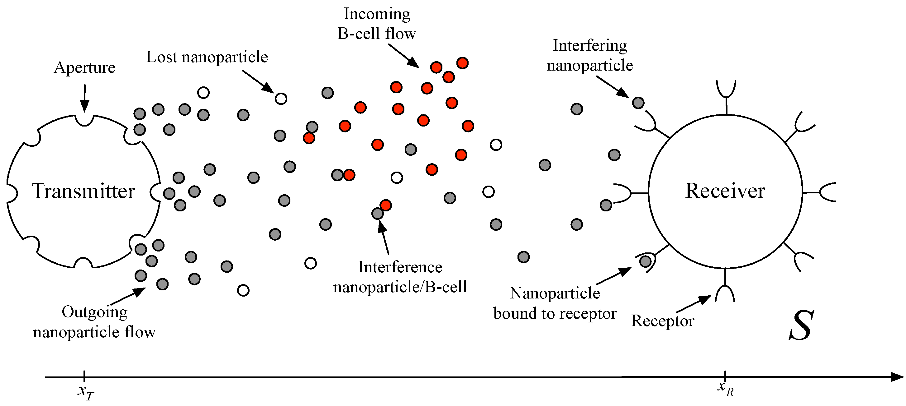
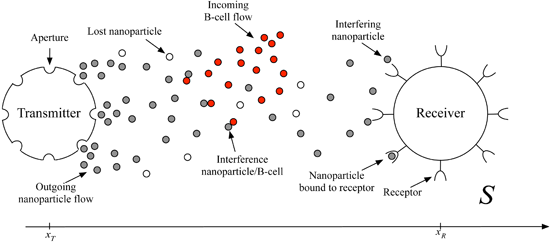
Similarly to [42], we consider a single nanoparticle as an indivisible object, released to (during the emission process) or collected from (during the reception process) a position in the space S, by means of chemical reactions. In the diffusion process, nanoparticles are free to move into the space following the laws of diffusion of particles in a flow. Figure 1 depicts a schematic of the end-to-end model in a biological environment, where a transmitting nanomachine emits a flux of nanoparticles toward a receiver. Notice that the receiver modeling is not addressed in this paper, since the aim is the modeling of the human immune system and how it affects the nanoparticulate drug delivery system.

Figure 1. End-to-end physical model in the biological space S, linking a transmitting nanomachine to a receiver. One or more fluxes of nanoparticles are emitted by the transmitter and diffuse along the propagation channel. The presence of B-cells causes a reduction of the nanoparticle concentration able to reach the receiver, modeled as fixed nodes in the nanonetwork. Moreover, lost and interfering nanoparticles can provide errors during the reception process (i.e., no reception and missing reception, respectively).

Figure 1. End-to-end physical model in the biological space S, linking a transmitting nanomachine to a receiver. One or more fluxes of nanoparticles are emitted by the transmitter and diffuse along the propagation channel. The presence of B-cells causes a reduction of the nanoparticle concentration able to reach the receiver, modeled as fixed nodes in the nanonetwork. Moreover, lost and interfering nanoparticles can provide errors during the reception process (i.e., no reception and missing reception, respectively).

The nanomachine is provided with several apertures from which the nanoparticles are emitted. The overall nanoparticle concentration flux emitted by the nanomachine is stimulated by a concentration gradient between $c_{out}$ and $c_{in}$, which represent the nanoparticle concentration value outside and inside the nanomachine, respectively. Specifically, the particle concentration inside the nanomachine is triggered according to increases (decreases) of the input signal, which allows the transmitter to increment (reduce) $c_{in}$, and then, the particle concentration at the output $c_{out}$ is increased (decreased), as well. Notice that we assumed only a positive nanoparticle rate modulation, i.e., $c_{in}<c_{out}$, [43].

A single nanoparticle is functionalized to be captured by a receptor, by means of chemical reactions. When captured, the reception process allows decoding the information within the nanoparticle (e.g., the drug concentration).

In the space S within the biological environment, we assume the presence of B-cells, which can recognize neighboring nanoparticles as antigens and then will try to defeat them (i.e., interference nanoparticle/B-cell). Finally, along the biological channel, we consider the presence of errors, expressed in terms of lost and interfering nanoparticles.

The overall nanoparticle concentration flux $J_T\left(x,t\right)$ is given by the sum of the N nanoparticle concentration gradients i.e., with N as the number of apertures of the nanomachine, at time t and position x through Fick’s first law (we recall that ∇ is an operator used in vector calculus as a vector differential operator), as follows:

$$J_T\left(x,t\right)=-D\sum _{i=1}^N\nabla C_{i,NP}\left(x,t\right)$$

(7)

and at the transmitter side (i.e., at position $x=x_T$ (nm) and time instant $t=t_0$ (ns), it becomes:

$$J_T\left(x_T,t_0\right)=-D\sum _{i=1}^N\nabla C_{i,NP}\left(x_T,t_0\right)$$

(8)

where $C_{i,NP}(x,t)$ (mol/cm${}^3$) is the i-th nanoparticle concentration with $i=\{1,2,\cdots ,N\}$ and D (cm${}^2$/s) is the diffusion coefficient, assumed as a constant value for a given fluidic medium and depending on the size and shape of nanoparticles, as well as the interaction with the solvent and viscosity of the solvent. Notice that the nanoparticle transmission rate $r_T\left(t\right)$ can be identified with Equation (8), due to the dependance on the concentration gradient.

Unfortunately, Fick’s first law works when applied to steady-state systems, namely the concentration will keep constant both along space and in time. However, since nanoparticles diffuse along space, the concentration changes during time, and they determine different levels of concentration. Then, we can rely on Fick’s second law, i.e.:

$$\frac{\delta C_{NP}\left(x,t\right)}{\delta t}=D\frac{{\delta }^2{C}_{NP}\left(x,t\right)}{\delta x^2}$$

(9)

where $C_{NP}$ is the nanoparticle concentration as emitted by the transmitter.

During the diffusion process, we consider that the nanoparticles encounter the B-cells. Due to comparable sizes, we can model the B-cells by means of Fick’s first and second laws, as considered for the nanoparticles. Under this assumption, the interactions among B-cells and the nanoparticles can occur, thus affecting nanoparticle flows. Indeed, analogously to Equation (8), we can model the B-cell concentration flux $J_B(x,t)$ as a unique contribution, which is expressed as:

$$J_B\left(x,t\right)=-D_B\nabla C_B\left(x,t\right)$$

(10)

where $C_B(x,t)$ is the B-cell concentration at position x and at time t and $D_B$ (cm${}^2$/s) is the diffusion constant for the B-cells (i.e., with $D_B\ne D$). Furthermore, from Equation (9) we can derive the B-cell diffusion along space x and at time t as:

$$\frac{\delta C_B\left(x,t\right)}{\delta t}=D_B\frac{{\delta }^2{C}_B\left(x,t\right)}{\delta x^2}$$

(11)

Due to the phagocytosis process of the immune system, the B-cell flux interacts with the nanoparticles, thus providing a reduction of nanoparticle concentration flux. The interaction among B-cells and nanoparticles allows writing the following:

$$J_{\left[T+B\right]}\left(x,t\right)=\frac{J_T\left(x,t\right)+J_B\left(x,t\right)}{2}$$

(12)

where we assumed:

$$J_T\left(x,t\right)=\frac{Q_{NP}}{\sqrt{{\left(4\pi Dt\right)}^3}}{e}^{-\frac{x^2}{4Dt}}$$

(13)

and:

$$J_B\left(x,t\right)=\frac{Q_B}{\sqrt{{\left(4\pi D_{B}t\right)}^3}}{e}^{-\frac{x^2}{4D_{B}t}}$$

(14)

with $Q_{NP/B}$ as the initial concentration of nanoparticles and B-cells, respectively. Equation (12) represents the nanoparticle concentration flux after the phagocytosis process, and it can be rewritten as:

$$J_{\left[T+B\right]}\left(x,t\right)=\frac{1}{2\sqrt{{\left(4\pi t\right)}^3}}\left[\frac{Q_{NP}}{D\sqrt{D}}{e}^{-\frac{x^2}{4Dt}}+\frac{Q_B}{D_B\sqrt{D_B}}{e}^{-\frac{x^2}{4D_{B}t}}\right]$$

(15)

When considering the circulatory system, it is more appropriate to consider a model that takes into account drift into the diffusion process. Let us suppose that the fluid is flowing with a constant drift velocity v (i.e., $v>0$); the diffusion equation in the medium would be:

$$J_T\left(x,t\right)=\frac{Q_{NP}}{\sqrt{{\left(4\pi Dt\right)}^3}}{e}^{-\frac{{(x-v)}^2}{4Dt}}$$

(16)

where we consider that the pdf of the position of a single particle, for every t, has a Gaussian distribution, i.e.,

$$P\left(x,t\right)=\frac{1}{\sqrt{4\pi Dt}}{e}^{-\frac{{(x-v)}^2}{4Dt}}$$

(17)

However, it is worth noticing that the basic model (namely, without the drift) has been considered as the reference model for developing a future in vitro experiment to validate our interference system.

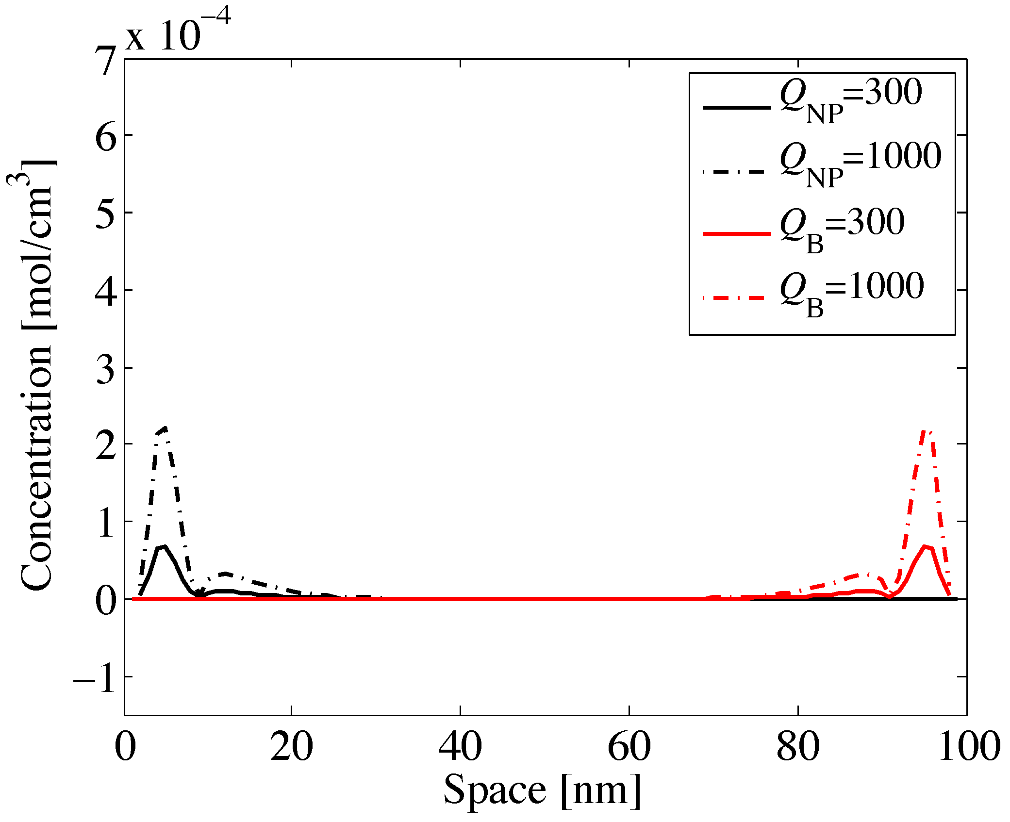
Figure 2 depicts the concentrations of nanoparticles and B-cells, occurring along space, by assuming the nanoparticles are emitted in position $x_T=0$ (nm), while the B-cells in position $x_B=99$ (nm). The flows diffuse in the opposite direction, i.e., from left to right for the nanoparticles and from right to left for the B-cells. Different curves are for different values of $Q_{NP/B}$, specifically for $Q_{NP/B}=300$ (mol) (solid lines) and $Q_{NP/B}=1000$ (mol) (dotted lines). Numerical values are chosen as a practical example.

Figure 2. Variation of nanoparticle and B-cell concentrations vs. space and for different values of initial concentration $Q_{NP/B}$.

Figure 2. Variation of nanoparticle and B-cell concentrations vs. space and for different values of initial concentration $Q_{NP/B}$.

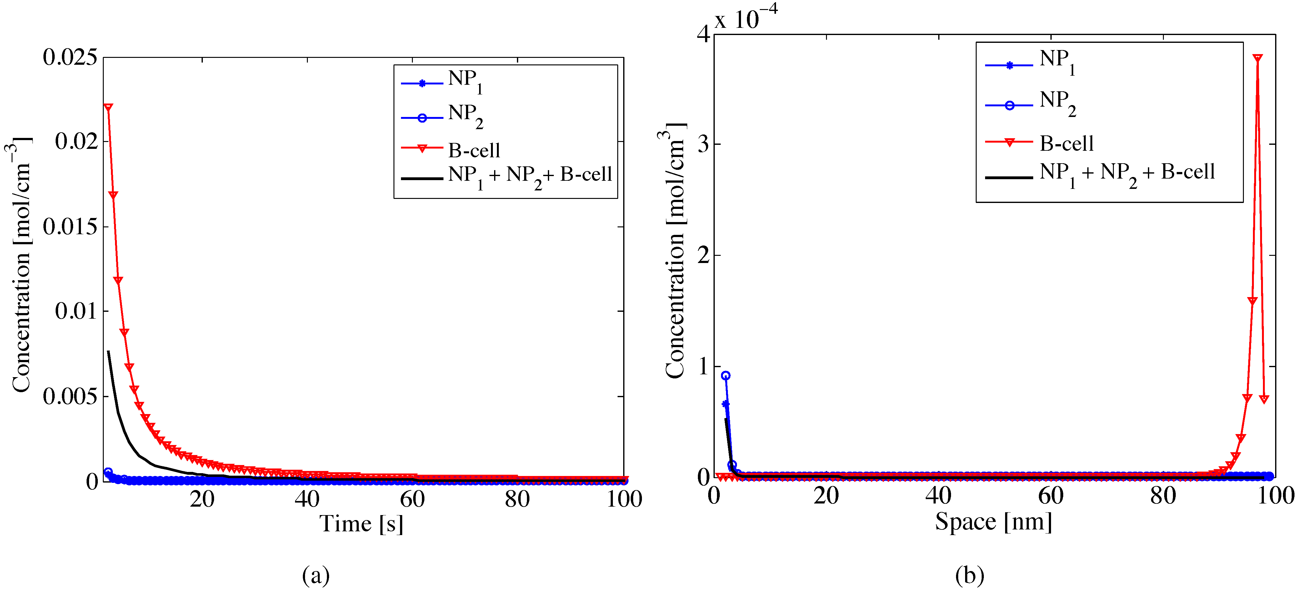
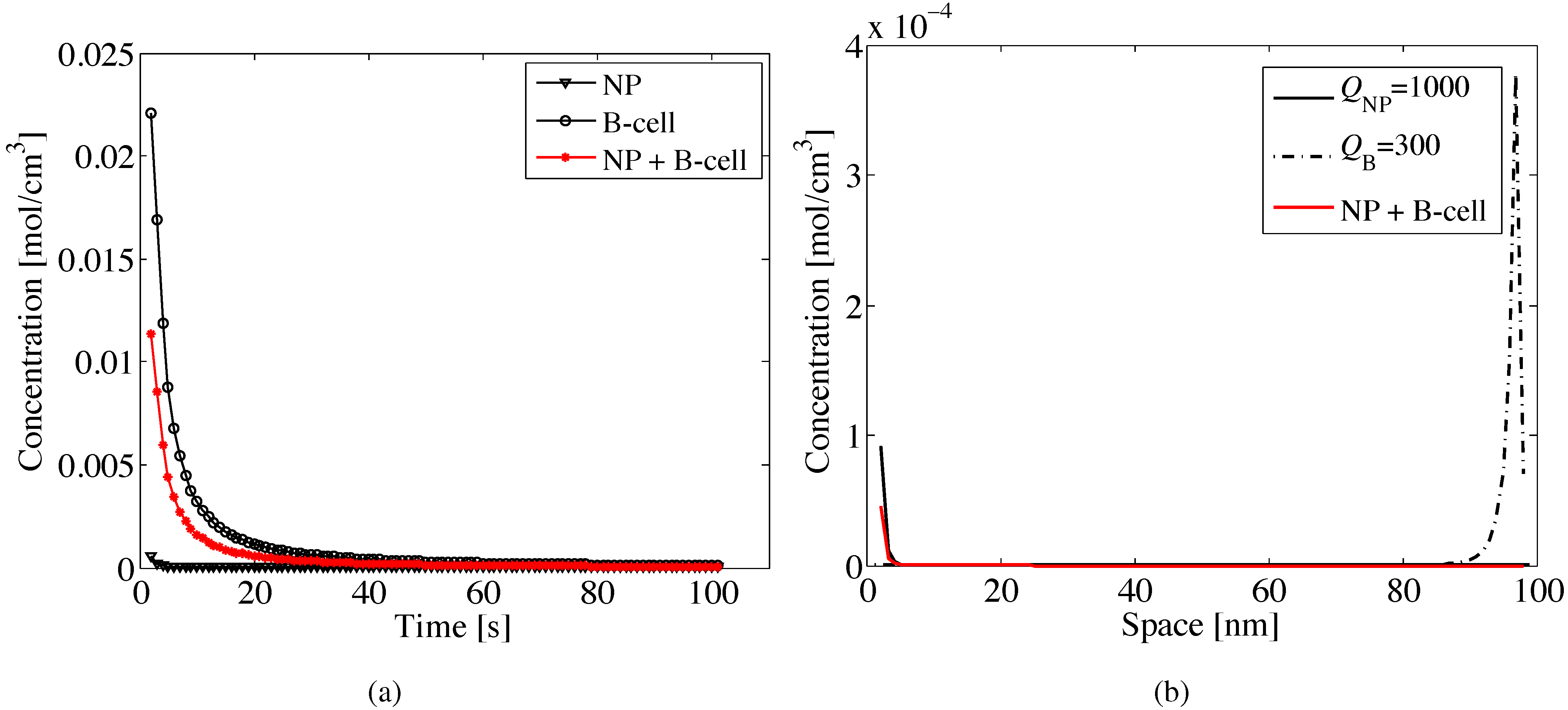
The interaction among nanoparticles and B-cell vs. space is shown in Figure 3a, where we observe how the flow of nanoparticles decreases due to the response of the immune system that recognizes the nanoparticles as invaders.

We assume the nanoparticles move at $1.13\times {10}^3$ (nm${}^2$/s) and the B-cells at $16.21$ (nm${}^2$/s). Those values have been obtained based on the well-known formula of the diffusion coefficient that is related to the hydrodynamic size of the particles, i.e.,

$$D=\frac{k_B·T}{3\pi \eta d}$$

(18)

where $k_B$ is the Boltzmann constant equal to $1.38\times {10}^{-23}J/K$, T is the temperature expressed in Kelvin, η is the viscosity of the liquid (m Pa ·s) and d is the size of the nanoparticles (B-cell) in (nm) (in (μm), respectively). Specifically, we assumed that the liquid is at the temperature of $37{}^{\circ }$C and the viscosity of the blood is $4.0$ (m Pa ·s).

After the phagocytosis process, the percentage of nanoparticles able to reach the receiver (i.e., NP + B-cell flow) will be lower than that in the case of no response of the immune system (i.e., NP flow). Indeed, if in space the concentration of B-cells is low (i.e., approximable to zero), there will be no response of the immune system and then no decrease of the nanoparticle concentration. Finally, Figure 3b depicts the dynamic behavior of the nanoparticle flow vs. space, when affected by the B-cell concentration (i.e., after the phagocytosis process). We observe a decrease of nanoparticle concentration flow due to the response of the immune system. This shows that in a real scenario, during the diffusion process, the nanoparticle concentration flow does not follow an ideal behavior, but is affected by other molecules (i.e., the B-cells), which destroy the nanoparticles, since they are recognized as pathogens.

Figure 3. Variation of nanoparticle and B-cell concentrations vs. (a) time and (b) space for different values of initial concentrations, i.e., $Q_{NP}=1000$ (mol) and $Q_B=300$ (mol). We assumed specific sizes for nanoparticles and B-cells. The superposition effect provides the average concentration due to the interaction among nanoparticles and B-cells (i.e., NP + B-cell).

Figure 3. Variation of nanoparticle and B-cell concentrations vs. (a) time and (b) space for different values of initial concentrations, i.e., $Q_{NP}=1000$ (mol) and $Q_B=300$ (mol). We assumed specific sizes for nanoparticles and B-cells. The superposition effect provides the average concentration due to the interaction among nanoparticles and B-cells (i.e., NP + B-cell).

3.1. Multi-Source Nanoparticulate Scenario

After describing the behavior of B-cells when a single-source nanoparticle flow is injected into the human body, we analyze a multi-source scenario, considering the emission of two nanoparticle flows at different diffusion coefficients. This particular scenario represents the case of the injection of different nanoparticles flows for therapeutic applications.

Figure 4a depicts the concentration behavior for two flows of nanoparticles (i.e., NP${}_1$ and NP${}_2$) moving at $1.41\times {10}^3$ nm${}^2$/s and $1.13\times {10}^3$ nm${}^2$/s, respectively. Again, we assume the B-cells diffuse at $16.21$ nm${}^2$/s. We then evaluated the immune system response, computed as the average trend given by the two nanoparticle flows and the B-cells. This response is then assessed versus space in Figure 4b. Similarly to Figure 2, we observe that the nanoparticle flows (i.e., red and blue lines) diffuse in opposite directions, and the immune system response (i.e., black line) is almost null along the end-to-end distance from the transmitter at 0 nm to the receiver laying at 99 nm.

Figure 4. Variation of nanoparticles and B-cell concentrations, vs. (a) time and (b) space for different values of initial diffusion coefficients i.e., $1.41\times {10}^3$ (nm${}^2$/s) for NP${}_1$, $1.13\times {10}^3$ (nm${}^2$/s) for NP${}_2$ and $16.16$ (nm${}^2$/s) for B-cells. The superposition effect provides the average concentration due to the interaction among two flows of nanoparticles and the B-cells (i.e., NP${}_1$ + NP${}_2$ + B-cell).

Figure 4. Variation of nanoparticles and B-cell concentrations, vs. (a) time and (b) space for different values of initial diffusion coefficients i.e., $1.41\times {10}^3$ (nm${}^2$/s) for NP${}_1$, $1.13\times {10}^3$ (nm${}^2$/s) for NP${}_2$ and $16.16$ (nm${}^2$/s) for B-cells. The superposition effect provides the average concentration due to the interaction among two flows of nanoparticles and the B-cells (i.e., NP${}_1$ + NP${}_2$ + B-cell).

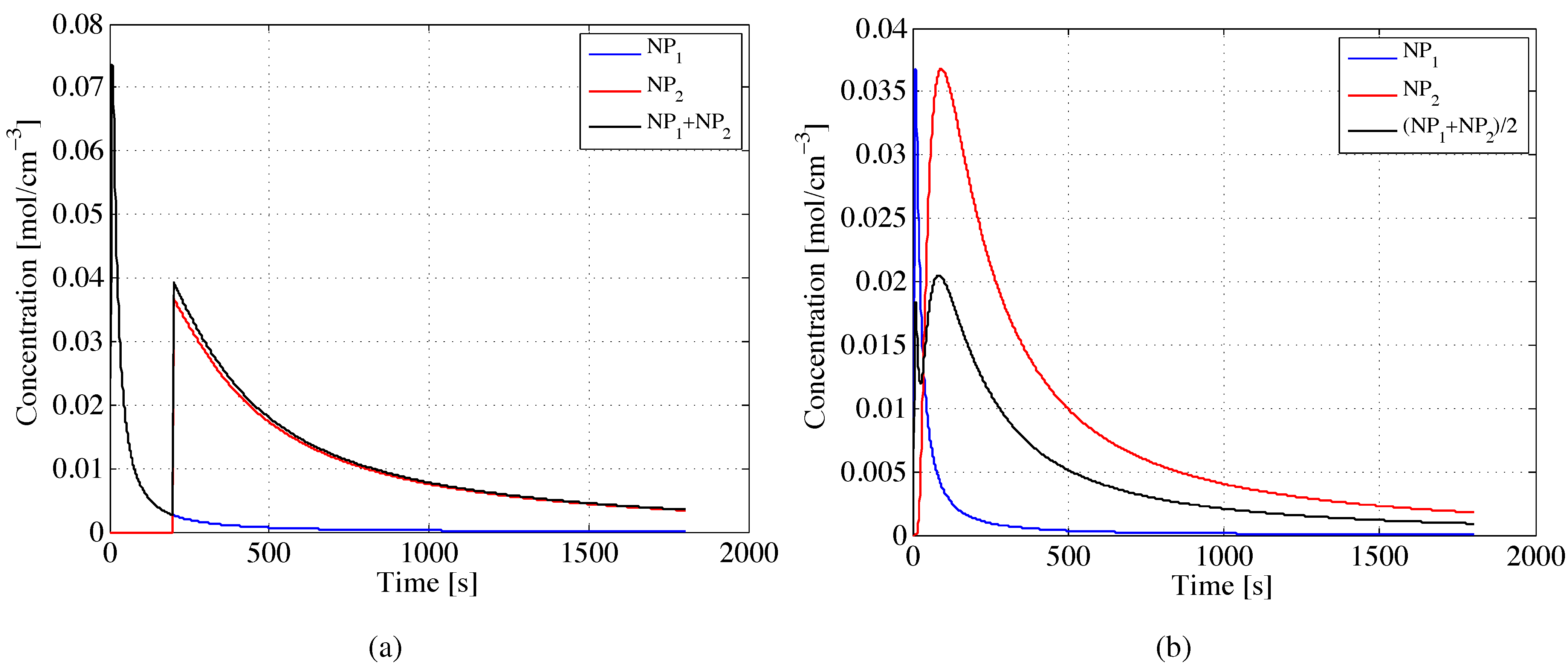
The concept of synchronous and asynchronous nanoparticle emission takes place when adopting a multi-source nanoparticle scenario. In the case of asynchronous nanoparticle emission, we assume the emission of NP${}_1$ nanoparticle flow starts at $t=t_1$ s, while NP${}_2$ nanoparticle flow starts at $t=t_2$ s with $t_2>t_1$. As a consequence, the resulting flow $J_{\mathrm{NP}}(x,t)$ is given as the sum of the two single flows, such as:

$$J_{\mathrm{NP}}(x,t)=J_{{\mathrm{NP}}_1}(x,t)+J_{{\mathrm{NP}}_2}(x,t)$$

(19)

Figure 5a depicts the concentration trend in the case of asynchronous nanoparticle emission versus time, where the initial concentrations are the same (i.e., $Q=1000$), and the diffusion coefficients for NP${}_1$ and NP${}_2$ flows are respectively 2 and $0.18$ (nm${}^2$/s). On the other hand, Figure 5b shows the emission of NP${}_1$ and NP${}_2$ nanoparticle flows in synchronous mode, where the resulting flow $J_{\mathrm{NP}}(x,t)$ is given as the average of the two single flows, such as:

$$J_{\mathrm{NP}}(x,t)=\frac{J_{{\mathrm{NP}}_1}(x,t)+J_{{\mathrm{NP}}_2}(x,t)}{2}$$

(20)

In this case, the nanoparticle emission occurs in the same time instance, and it results as the emission of a single flow obtained as the average of $J_{{\mathrm{NP}}_1}$ and $J_{{\mathrm{NP}}_2}$.

Figure 5. Nanoparticle concentrations for two flows NP${}_1$ and NP${}_2$ emitted in (a) asynchronous and (b) synchronous mode. The resulting concentrations are depicted in black.

Figure 5. Nanoparticle concentrations for two flows NP${}_1$ and NP${}_2$ emitted in (a) asynchronous and (b) synchronous mode. The resulting concentrations are depicted in black.

4. Nanoparticle Errors

Apart from the presence of B-cells that can cause a reduction of nanoparticle concentration, we can distinguish other errors occurring in our nanoparticulate system during the diffusion process, namely (i) the interfering nanoparticles, i.e., nanoparticles that can approach the receiver, but are not able to form bindings and cause interference and (ii) the lost nanoparticles, i.e., nanoparticles that are not able to reach the receiver, since they are lost during the diffusion process.

Interfering nanoparticles provide an increase of the noise level in the channel, causing a missing reception, since they can lay very close to the receiver, then obstructing other nanoparticles from the correct capture at the receptor. In this context, a missing reception means that a nanoparticle lays very close to the receptor, but is not bound. On the other side, lost nanoparticles will never reach the receiver and then will provide no reception, since no correct nanoparticle capture will occur. In this context, no reception means that a nanoparticle will never form a binding, since it will not reach the receiver.

Based on such errors, we can distinguish two kinds of events, such as (i) the individual and correlated simultaneous nanoparticle faults and (ii) the interference-based nanoparticle faults. In the case of individual nanoparticle faults, at least one nanoparticle out of a nanoparticle flow is affected by noise, and then, the nanoparticle reception at the receiver can be corrupted. Finally, the case of correlated simultaneous nanoparticle faults represents the extension of individual faults, since it assumes errors correlated among multiple nanoparticle flows.

4.1. Individual and Correlated Simultaneous Nanoparticle Errors

We can define p as the probability of having one failed nanoparticle, i.e., $N{P}_f=1$ (specifically, one lost nanoparticle), out of $N_{NP}$ nanoparticles, whose expression is:

$$p[N{P}_f=1]\cong N_{NP}·P_{NPf},\mathrm{with}{P}_{NPf}\ll 1$$

(21)

where $P_{NPf}$ is the rate of nanoparticle faults. It follows that the probability p of having two failures out of $N_{NP}$ nanoparticles is:

$$p[N{P}_f=2]=\left(\begin{array}{c}{N}_{NP}\\ 2\end{array}\right)P_{NPf}^2·{\left(1-P_{NPf}\right)}^{N_{NP}-2}$$

(22)

and then, the probability of having three or more failures is:

$$p\left[N{P}_f>2\right]=\sum _{l=3}^{N_{NP}}{P}_{NPf}^l·{\left(1-P_{NPf}\right)}^{N_{NP}-l}$$

(23)

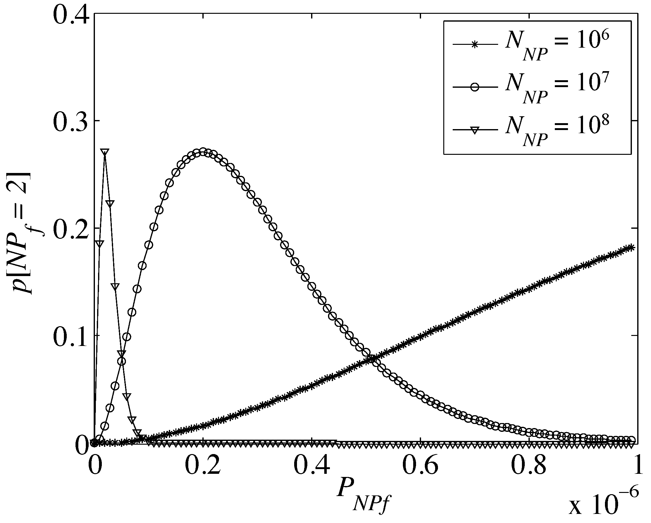
As an example, for $P_{NPf}={10}^{-6}$, we obtain $p\left[N{P}_f=2\right]=0.183$ in the case of $N_{NP}={10}^6$, while the probability decreases (i.e., $p\left[N{P}_f=2\right]=0.0023$) in the case of $N_{NP}={10}^7$. Figure 6 depicts the nanoparticle fault probability for different values of fault probability of a single nanoparticle out of $N_{NP}$, for $N_{NP}=[{10}^6,{10}^7,{10}^8]$.

Figure 6. Probability of having two failed nanoparticles out of a flow of $N_{NP}={10}^6$ (asterisk), $N_{NP}={10}^7$ (circle) and $N_{NP}={10}^8$ (upward-pointing triangle).

Figure 6. Probability of having two failed nanoparticles out of a flow of $N_{NP}={10}^6$ (asterisk), $N_{NP}={10}^7$ (circle) and $N_{NP}={10}^8$ (upward-pointing triangle).

Notice that it is realistic to assume that the probability of correlated simultaneous nanoparticle faults (i.e., $P_{cNPf}$) can exceed the individual fault probability (i.e., $P_{sNPf}$). On the other hand, when m nanoparticle flows are considered, the probability that at least one flow is not affected by a correlated failure (i.e., $m_{healthy}\ge 1$) is:

$$Pr\left\{m_{healthy}\ge 1\right\}=1-P_{cNPf}^m$$

(24)

Thus, for $P_{cNPf}={10}^{-6}$ with $m=3$ nanoparticle flows, the probability that at least one flow is not affected by correlated faults is less than $\left(1-{10}^{-18}\right)$.

4.2. Interference-Based Nanoparticle Faults

This case occurs due to interference errors along the channel from the transmitter to the receiver. When the nanoparticles diffuse, an additional delay can happen, mainly due to the presence of obstacles in a lattice, i.e., a three-dimensional space. This corresponds to the nanoparticle to “surf” in a perpetual way until this is eliminated by the human body. In this case, a missing reception can still arise due to large random errors produced during the reception process (i.e., interfering nanoparticles that are laying near the receptors, but that are not bound). Indeed, a great part of the desired particles will not be able to reach the surface receptors of the receiver node, and at the same time, the interfering particles will not be compatible with the surface receptors. Then, there will be no reception. However, besides their small probability of occurrence, interfering nanoparticles can cause a missing reception, due to the very short proximity of these nanoparticles to the receptors.

Let us denote with $P_{sNPf}$ the probability of the fault of a single nanoparticle and with $N_{NP}$ the number of nanoparticles available at the end of the diffusion process. The probability p that none of them is affected by a fault (i.e., the nanoparticles can form bindings and are not interfering) is bounded by the probability that none of them is affected by an independent fault, i.e.:

$$p\le {(1-P_{sNPf})}^{N_{NP}}$$

(25)

In practice, for $P_{sNPf}\ll 1$, the following approximation holds:

$$p\le 1-N_{NP}·P_{sNPf}$$

(26)

We need to compute the conditions under which this approximation is true. In order to do that, we will derive a free boundary problem for the associate Fokker–Planck partial differential equation, which is derived from the calibration of the barrier function [44].

Let us define the function $P_{sNPf}\left(t\right)$ as the probability that a single nanoparticle has faulted by time t, and $P_{sNPf}^{\prime }\left(t\right)$ as the fault probability density. Then, the probability of fault between t and $(t+\Delta t)$ can be represented as $P_{sNPf}^{\prime }\left(t\right)\Delta t$, as seen at time $t=0$.

By considering $W\left(t\right)$ as a standard Wiener process, we can associate the nanoparticle concentration process as an Ito process [45] $X=\{X_t,t\ge 0\}\left(t\right)$, with $X_{t=0}=X_0$. The reasons for which we associate an Ito process to our system is that an Ito process is a stochastic process that can be expressed as the sum of an integral with respect to Brownian motion and an integral with respect to time, as shown in:

$$X_t=X_0+\underset{0}{\overset{t}{\int }}a\left(X_s,s\right)ds+\underset{0}{\overset{t}{\int }}b\left(X_s,s\right)d{W}_s,t\ge 0$$

(27)

where $X_0$ is a scalar starting point and $\left\{a\left(X_t,t:t\ge 0\right)\right\}$ and $\left\{b\left(X_t,t:t\ge 0\right)\right\}$ are stochastic processes satisfying certain regularity conditions. The terms $a\left(X_t,t\right)$ and $b\left(X_t,t\right)$ are the drift and the diffusion, respectively. A solution of Equation (27) is:

$$d{X}_t=a_{t}dt+b_{t}d{W}_t$$

(28)

where $a_t=a\left(X_t,t\right)$ and $b_t=b\left(X_t,t\right)$. Equation (28) represents the expression of Brownian motion with an instantaneous drift $a_t$ and an instantaneous variance $b_t^2$ of diffusion. The faults of the nanoparticles at time t are expressed through:

$$X\left(t\right)=b\left(t\right)$$

(29)

with the assumption that $X\left(t-1\right)>b\left(t-1\right)$, where $b\left(t\right)$ represents the barrier function related to the density of nanoparticles present in the solution.

Let us call τ the first time that $X\left(t\right)$ hits its barrier, then:

$$\tau =inf\left\{t\ge 0:X\left(t\right)\le b\left(t\right)\right\}$$

(30)

By calling $P_S(x,t)$ the survival probability density function of $X\left(t\right)$, we have:

$$P_S\left(x,t\right)dx=Pr\left[x<X\left(t\right)<x+dx,\tau \ge t\right]$$

(31)

for $x\ge b\left(t\right)$. Then, by applying the results known in the theory of probability, the function $P_S(x,t)$ in Equation (31) satisfies the Fokker–Planck equation, such as:

$$\frac{\partial P_S\left(x,t\right)}{\partial t}=\frac{{\sigma }^2}{2{\gamma }^2}\Delta P_S\left(x,t\right)+\frac{F\left(x\right)}{\gamma }\nabla P_S\left(x,t\right)$$

(32)

where $\frac{{\sigma }^2}{2{\gamma }^2}=D$ is the diffusion coefficient, γ is a viscosity coefficient and $F\left(x\right)$ is a strength field. From Equation (25), we can define the survival probability up to time t corresponding to $\left(1-P_{sNPf}\left(t\right)\right)$ and calculated by integration as:

$$1-P_{sNPf}\left(t\right)=\underset{b\left(t\right)}{\overset{\infty }{\int }}{P}_S\left(x,t\right)dx$$

(33)

so that the fault probability $P_{sNPf}\left(t\right)$ is related to the survival probability density function $P_S(x,t)$ and the barrier $b\left(t\right)$ through the following equation:

$$P_{sNPf}\left(t\right)=1-\underset{b\left(t\right)}{\overset{\infty }{\int }}{P}_S\left(x,t\right)dx$$

(34)

Since the pair $\{P_S(x,t),b\left(t\right)\}$ has to be consistent with the fault probability $\{P_{sNPf}\left(t\right);t>0\}$, the barrier $b\left(t\right)$ has to be chosen in an appropriate fashion. This is clear by differentiating the fault probability with respect to time in Equation (34):

$$\begin{array}{cc}{P}_{sNPf}\left(t\right)\hfill & =-\underset{b\left(t\right)}{\overset{\infty }{\int }}\frac{\delta P_S}{\delta t}dx+P_S\left[b\left(t\right),t\right]b^{\prime }\left(t\right)\hfill \\ & =\frac{1}{2}\frac{\delta }{\delta x}{\left.\left({\sigma }^2{P}_S\right)\right|}_{x=b\left(t\right)}\hfill \end{array}$$

(35)

In practice, the survival density function has to satisfy both Condition (33), and a boundary condition at the barrier $x=b\left(t\right)$. This implies a free boundary problem for the forward Fokker–Plank equation, since the boundary $b\left(t\right)$ is not known and the choice of its value has to be consistent with the boundary Conditions (33) and (35). Notice that the derived model is invariant with respect to transformation as scaling. Indeed, by introducing $s_0$ as a positive number and transforming $\tilde{x}=x/s_0$, $\tilde{b}\left(t\right)=b/s_0$ and $\tilde{a}\left(\tilde{x},t\right)=a\left(x,t\right)/s_0$, then the new function can be written as:

$${\tilde{P}}_S\left(\tilde{x},t\right)=s_0{P}_S\left(x,t\right)$$

(36)

that satisfies Equations (32)–(35). Finally, if $s_0$ is a constant value, i.e., $\left(s_0=1\right)$, the fault index is taken to be a standard Brownian motion. On the other side, if $s_0$ is not constant, we can also take into account the index as time.

From the navigation theory [46,47], we take the concept of protection level [48] and adapt it to our system. Specifically, we assume it as the event that there is at most one in ten million chance that the detection error is greater than the protection level (PL). The intention behind this is to keep the probability of hazardous situations (i.e., faulty nanoparticles) extremely low. Indeed, when every nanoparticle is healthy, denoting by ${\sigma }_d^2$ the variance of the detection error, modeled as a Gaussian random variable (r.v.), and η its expectation, then the conditional probability of a misleading information (MI) event, given a missing alert (MA) event, equals the probability that the detection error $\Delta E$ will exceed the protection level $PL$. Basically, we obtain:

$$\begin{array}{cc}{P}_f\left(\left.MI\right|MA\right)\hfill & =Pr\left\{\Delta E>PL\right\}\hfill \\ & =\frac{1}{2}erfc\left(\frac{PL-\eta }{\sqrt{2}{\sigma }_d}\right)+\frac{1}{2}erfc\left(\frac{PL+\eta }{\sqrt{2}{\sigma }_d}\right)\hfill \end{array}$$

(37)

where $erfc\left(·\right)$ is the complementary error function, defined as:

$$erfc\left(x\right)=\frac{2}{\sqrt{\pi }}\underset{x}{\overset{\infty }{\int }}{e}^{-t^2}dt$$

(38)

5. Hazardous Misleading Information Rate

After describing all of the cases for nanoparticle errors, we can now derive the hazardous misleading information (HMI) rate. Again, from the navigation theory, we use the concept of the HMI event that occurs when the detection error exceeds the alert limit, i.e., for a given parameter measurement, the alert limit is the error tolerance not to be exceeded without issuing an alert. In our case, the alert represents the event that a nanoparticle is considered healthy while it is not. This kind of analysis will be very useful in order to characterize the different types of misleading information and o analyze their effect on the whole system.

Let us denote by $P_{MA}^{NPH}$ the missing alert probability when all of the nanoparticles of a given flow are healthy and $P_{MA}^{NPF}$ as the missing alert probability when at least one nanoparticle of a given flow is faulty. Notice that the acronyms $MA$, $MI$, $NPH$ and $NPF$ are given in Table 1. Moreover, $P_{MI/MA}^{NPH}$ is the conditional probability of an $MI$ event given an $MA$ event, when all of the nanoparticles of a given flow are healthy and $P_{MI/MA}^{NPF}$ the conditional probability of an $MI$ event given an $MA$ event when at least one nanoparticle of a given flow is faulty. Then, $N_{Dec}$ is the number of independent decisions in a given time interval, i.e., one hour [49]. $P_{NPH}$ is the probability that all of the nanoparticles are healthy, and $P_{NPF}=1-P_{NPH}$ is the probability that at least one nanoparticle is faulty.

Then, the hazardous misleading information rate $R_{HMI}$ is evaluated as the probability of an HMI event in one hour, such as:

$$R_{HMI}=1-\left\{{\left[1-P_{MI}^{NPH}\right]}^{N_{Dec}}·P_{NPH}+{\left[1-P_{MI/MA}^{NPF}{P}_{MA}^{NPF}\right]}^{N_{Dec}}·P_{NPF}\right\}$$

(39)

Roughly speaking, the hazardously misleading information (and then, the computation of the rate of the probability of the hazardous misleading information) will give important information about the integrity requirements of the system. Based on the different potential applications in nanomedicine, the “integrity” definition could assume different values, but in any case, it would represent a very important point to be fixed. Notice that, in principle, the integrity risk [50] is proportional to the square of the bias introduced by the nanoparticle failure. Thus, the hazardous misleading information rate should be averaged even with respect to this quantity. However, since a reliable statistical model for the entity of the errors caused by nanoparticle failures is not available, the protection level should be set in accordance to the worst case.

Table 1. Acronyms used for the computation of the hazardous misleading information (HMI) rate.

Acronym	Event Type
$MA$	Missing alert event
$MI$	Misleading information event
$NPH$	Event corresponding to healthy nanoparticles
$NPF$	Event corresponding to one or more uncorrelated nanoparticle failure

Table 1. Acronyms used for the computation of the hazardous misleading information (HMI) rate.

Acronym	Event Type
$MA$	Missing alert event
$MI$	Misleading information event
$NPH$	Event corresponding to healthy nanoparticles
$NPF$	Event corresponding to one or more uncorrelated nanoparticle failure

6. Related Work

One major obstacle for the use of nanoparticles in in vivo applications is the rapid clearance by the cells of the immune system. Several contributions have tried to address the issue of the interaction between the nanoparticulate system and the immune system. In [22], the authors outline the importance to avoid extensive immunostimulatory or immunosuppressive reactions to the nanomaterials when injected in the body.

A deep comprehension of the interactions among the two systems, namely the nanoparticulate and the immune one, would be very useful to decree the success of nanomedicine. In order to study this specific aspect, the authors in [22] focus on Ag nanoparticles. In [51], the authors focus on the observations related to two specific immune correlated “activities”, such as immunostimulation and immunosuppression. They consider that particle properties may generate specific interactions with the immune cells.

An initial study on the phagocytosis effect of immune cells has been done in [52]. The authors show how different properties can “stimulate” different responses and also have an impact on the biodistribution of the nanoparticles. They provide an overview of in vitro methods, useful in identifying interactions with the components of the immune system, and in particular, they focus on the nanoparticle distribution to tissues based on the effect of this type of interaction. The aim of the authors is very similar to our scope, but we approached it in a different way, since we rely on a general and a theoretical/statistical model.

Furthermore, in [53], the authors focus on the phagocytosis system and outline specific approaches, such as grafting polyethylene glycol onto particles (PEGylation), which may increase the survival or circulation time in the blood for the nanoparticles. The authors outline these nanoparticles as being still cleared, and the processes behind this clearance are not completely understood. They study different strains that can impact on the rate of clearance and identified the differences in nanoparticle clearance when different strains of mice were considered.

An interesting summary of the interaction between the immune system and metal-based nanoparticles is reported in [21], where the authors conclude that the interaction of nanomaterial with the immune system is attracting much attention, since the physicochemical properties of nanoparticles are of paramount importance for the immunological response. On the other side, differently from the contributions considered, in this work, we try to design a quite general and yet complex model that can be effectively used and exploited for inferring interesting information regarding the nanoparticulate clearance ratio.

7. Conclusions

In this paper, we analyzed the interaction of the human immune system with a nanoparticulate system by deriving the errors (i.e., lost and interfering nanoparticles) and the cases of misleading information. The human immune system is very complex, and the approach we considered in this work was a simplified mathematical model based on differential equations including also B-cells, in order to make the system as realistic as possible. The choice of the specific model was also “constrained” by the necessity to include spatio-temporal features of the immune response and the maturation process of the B-cells that compete with the nanoparticles to share the biological environment.

This specific analysis allows us to treat the cells deriving from an immune response as a kind of interferent. We derived the probability analysis for the cases of missing and no reception on the basis of the presence of nanoparticle errors (i.e., interfering and lost nanoparticles). Moreover, we also derived the analysis of misleading information by considering different types of events.

As future work, we aim to consider mobile nanomachines (e.g., a mobile transmitter nanomachine and a time-evolving diseased biological tissue as a receiver nanomachine), and then, we assume a mobility model, like Brownian motion, for the transmitter nanomachine. Furthermore, we plan to validate this model through some initial in vitro experiments that will allow us to follow the progression in terms of both the amount of errors and the specific type of error that occur. In vitro studies based on fractionated blood products have been used to evaluate the effect of NP on the circulating blood. Since the effect of a nanoparticulate system on the immunological functions (e.g., macrophages, dendrites, etc.) has been evaluated, we will rely on these results in order to infer complementary information, namely how the immune system impacts the effectiveness and concentration of nanoparticles.