Article

Uncalibrated Visual Servo Control of Magnetically Actuated Microrobots in a Fluid Environment

by
Jenelle Armstrong Piepmeier
1,*,
Samara Firebaugh
2 and
Caitlin S. Olsen
1
1
Systems Engineering, United States Naval Academy, 105 Maryland Avenue, Annapolis, MD 21402, USA
2
Electrical and Computer Engineering, United States Naval Academy, 105 Maryland Avenue, Annapolis, MD 21402, USA
*
Author to whom correspondence should be addressed.
Micromachines 2014, 5(4), 797-813; https://doi.org/10.3390/mi5040797
Submission received: 9 June 2014 / Revised: 19 July 2014 / Accepted: 12 September 2014 / Published: 26 September 2014

Abstract

:
Microrobots have a number of potential applications for micromanipulation and assembly, but also offer challenges in power and control. This paper describes an uncalibrated vision-based control system for magnetically actuated microrobots operating untethered at the interface between two immiscible fluids. The microrobots are 20 μm thick and approximately 100–200 μm in lateral dimension. Several different robot shapes are investigated. The robots and fluid are in a 20 × 20 × 15 mm vial placed at the center of four electromagnets. Pulse width modulation of the electromagnet currents is used to control robot speed and direction. Given a desired position, a controller based on recursive least square estimation drives the microrobot to the goal without a priori knowledge of system parameters such as drag coefficients or intrinsic and extrinsic camera parameters. Results are verified experimentally using a variety of microrobot shapes and system configurations.

Graphical Abstract

1. Introduction

Tetherless microrobots have been proposed for a number of applications including minimally invasive surgery and micromanipulation of micro gels for in vitro tissue culture [1]. Such microrobots, which are at dimensions of tens to hundreds of micrometers, are of comparable size to many biological structures, such as cells, and therefore are an enabling technology. A challenge facing microrobots is providing power and control. In particular, adapting macroscale control strategies to the microscale environment is not always straightforward. The physics of microscale operation does not always scale intuitively. For example, surface forces such as friction or viscous drag play a much larger role than volumetric forces such as magnetic attraction or inertial forces. Adding to the difficulty of the problem, drag forces at this scale can be difficult to model for complex microrobot device geometries.
Tetherless microrobot actuation has been achieved using a number of different power delivery methods including optical [2], electrostatic [3], thermal [4], ultrasonic [5] and electromagnetic [6]. A review of propulsion methods specific to swimming microrobots medical applications is given in [7]. Closed-loop control can be achieved with vision-based feedback of the microrobot position. Controller designs typically utilize a system model that characterizes the interaction between the applied forces (magnetic, drag, electrostatic, etc.) on the microrobot and the microrobot motion. A selected number of magnetically controlled systems are reviewed here with specific emphasis on the feedback control methods used and the tracking performance achieved.
Using a clinical magnetic resonance imaging (MRI) system, Tamaz et al. [8] develop a proportional-integral-derivative (PID) controller capable of navigating a 1500 μm ferromagnetic bead along a predefined path. They conclude that an adaptive controller would significantly decrease complications in the system and allow for more robust uses in the biomedical field.
Belharet et al. demonstrate a generalized predictive control (GPC) scheme to actuate a 500 μmneodymium sphere in an endovascular environment using Maxwell and Helmholtz coils in [9] achieving tracking errors on the order of 50–200 μm depending on the fluid composition and flow conditions.
In [10], Pawashe et al. demonstrate model-based learning controllers for 210 μm microbead manipulation using side-pushing by a magnetic 480 μm microrobot operating in a fluid. Microbeads are pushed to within one pixel (7.5 μm). Modeling includes flow velocities induced by the microrobot and equations of motion for the microsphere being manipulated.
Diller [11,12] uses multiple magnetic robots of the same design as [13] with geometric dissimilarities that resulted in differing responses to various frequencies. Planar path errors in [11] are on the order of 1000–1500 μm and three-dimensional (3D) control is achieved in [12] with path errors with less than 310 μm for 350 μm robot and 1500 μm robot.
In [14] Marino et al. compare an H controller with a PID controller for a linear uncertain dynamical model for electromagnetic steering control of a 1000 μm microrobot in low viscosity oil using the OctoMag system [15]. Tracking errors on the order of 270–490 μm are reported using the H controller. In another work by the same research group [16], Bergeles discusses the difficulties in localizing the position of the microdevice in the ocular environment due to complex optics and distortions. They propose a new projection model that allows localization of the microrobot for control with a proportional-derivative (PD) controller.
Using the MiniMag (Aeon Scientific, Zürich, Switzerland) system, Ghanbari [17] proposes time-delay estimation (TDE) control as a superior approach to H control for handling the many uncertainties present in modeling microrobot systems. Errors less than 200 μm are demonstrated for a microrobot consisting of a NdFeB cylinder permanent magnet of diameter 500 μm and length 1000 μm. The method does require the selection of controller gains for a particular configuration of the system.
Keuning [18] and Khalil [19] use a proportional-integral (PI) controller and waypoints generated by path planning algorithms to achieve planar navigation of paramagnetic 100 μm beads moving in water. Average errors ranged from 4.7 to 7.0 μm with standard deviations on the order of 2.0 μm.
Initial work [20] by the authors of this paper investigate simple linear model and demonstrated a proportional control strategy for electromagnetic actuation of various microrobot devices operating between fluid layers. Each microrobot design responds differently to the actuating magnetic fields required its own set of gains to compute the required duty cycle.
While varying in complexity, all of these works rely on system models of the various subsystem components including the microrobot device, the environment it is operating within, the actuation system, and the visual feedback system. The contribution of this work is the demonstration of an uncalibrated microrobot control scheme that uses uncalibrated visual feedback for an unmodeled system consisting of a microrobot device operating in a fluidic environment observed via a microscope and controlled by four electromagnets. In this paper, we characterize the performance of this strategy by varying a number of system parameters (microrobot device, magnification, target velocity, etc.) without changing any terms in the controller or utilizing configuration specific controller gains. Assumptions made based on the system components are presented in Section 2 and the image-based estimation and control are presented in Section 3. Experimental results are given in Section 4 for planar control of various 200 μm microdevices at various magnifications and system configurations. The experimental results include point-to-point motion and trajectory following with path errors ranging from 1.0 to 4.1 pixels in the image plane (4.1–40.5 μm in the workspace).

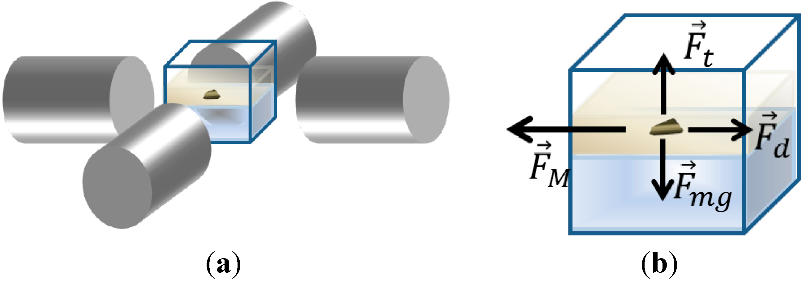
2. Electromagnetic Actuation for Microrobotic Control

For this work, we consider a ferromagnetic mass suspended in between two fluid layers and surrounded by two electromagnet pairs whose magnetic fields act primarily in the plane created by the fluid boundary as depicted in Figure 1a. This system was initially developed for participation in the Mobile Microrobot Challenge Competition [21]. While the method is extendable to higher degrees of freedom, for the theoretical and experimental results presented here it is assumed that there are two electromagnet pairs controlling a microrobot device that is acting in a planar, fluid environment.
As shown in Figure 1b, forces acting on this mass include electromagnetic forces F M , viscous drag F d , surface tension at the boundary F t , and apparent weight F w . Let x w represent the position of the mass, [ x y z   ] w T with respect to a fixed world coordinate frame. Then, the equation of motion for the mass is given by:
m x w ¨   = F d + F t + F w + F M
Further expanding the terms to include drag coefficients (α, β, γ) and the magnetic field strength ( B x ,   B y ,   B z ) results in:
m [ x ¨ y ¨ z ¨ ] w = [ α β γ ] [ x ˙ y ˙ z ˙ ] w + [ 0 0 F t + F w ] + [ M x || B x || M y || B y || M z || B z || ]
where M x represents the magnetic moment of the microrobot along the x-axis.
Figure 1. (a) Two electromagnet pairs arrayed about a ferromagnetic mass (the microrobot) operating in a fluid environment; and (b) the free body diagram of the microrobot in the fluid.
Micromachines 05 00797 g001
It is important to consider the relative magnitudes of the inertial and viscous forces acting on the body. The Reynolds number is a dimensionless quantity that relates inertial forces to viscous forces in the Navier-Stokes equations for a body moving in an incompressible Newtonian fluid. If the microrobot system is operating in a low Reynolds number regime (Re << 1), then the inertial term is much smaller than the drag forces as described by Purcell [22].
Furthermore, if we assume that the buoyant and surface tension forces counteract the gravitational forces, we have a microrobot operating in a planar region controlled by orthogonally oriented electromagnets. Thus, Equation (2) can be simplified for planar motion in a low Reynolds fluid environment as:
0 [ α β ] [ x ˙ y ˙ ] w + [ M x || B x || M y || B y || ]
As the microrobot motion is sensed by a computer vision system, the relationship between pixel coordinate frame and the world coordinate frame can be modeled using projective geometry and homogeneous coordinates. To relate microrobot velocities to pixel velocities, the image Jacobian Ji, sometimes called the interaction matrix, must be computed using partial derivatives where the elements of the matrix will be a function of the intrinsic and extrinsic camera parameters as well as the depth from the camera plane to the microrobot object. If planar robot motion is assumed, the following relationship is given where J i 2 × 2 :
[ x ˙ y ˙ ] p = J i [ x ˙ y ˙ ] w
Finally, combining Equations (3) and (4) the observed velocities (in pixels/s) of the microrobot are given by:
[ x ˙ y ˙ ] p J i [ M x α || B x || M y β || B y || ]
Thus, the fully modeled system would include camera parameters, drag coefficients, and magnetic field properties.
Since the magnetic field strengths are proportional to the applied current (generated by a pulse-width modulated voltage square wave), the system displays a linear relationship between the actuation signal, u ( t ) , the microrobot velocity   x ̇ p ( t ) (observed by the visual system) can be expressed as:
x ̇ p ( t ) J ( x )   u ( t )
where J ( x ) incorporates the image Jacobian together with the drag coefficients, magnetic moments, and magnetic field strengths. It is similar to the composite Jacobian matrix used in traditional image based robotic control and will similarly vary as the microrobot moves throughout the workspace. For the 2D system presented in this work, it is a 2 × 2 matrix that relates the actuation signal to the velocity of the microrobot as seen in the image plane.
Computing a closed form solution for J(x) is possible, but doing so requires accurate and calibrated models of the induced electromagnetic field, drag coefficients, the vision system, etc. Any changes to the physical position of the system, components, device geometry, fluid properties, etc. require a system calibration step. An alternative is online estimation of the J matrix using iterative methods such as Broyden’s method or recursive nonlinear least squares estimation. Such uncalibrated adaptive methods have been successfully implemented in macro-scale manipulators and mobile robots for a variety of applications with more complex nonlinear system models and higher degrees of freedoms (DOF) [23,24,25]. Experimental results in [20] and [26] show that the J matrix (the relationship between actuation and device velocities) is relatively linear for the experimental system used in this paper. The 2-DOF system described here presents a mathematically tractable problem for online system estimation as presented in the following section.

3. Uncalibrated Visual Servoing

3.1. Recursive Least Squares (RLS) Jacobian Estimation and Control

Consider a microrobot system such as the one described by Equation (6) with an observed state x that will vary when the control signal u n , is applied to the system. It is desired that the robot be controlled in such a manner that it is driven towards a goal position or trajectory x * ( t ) . The error f : m between the observed and desired or target position, x * ( t ) , is given by:
f ( x ( t ) ) = x ( t ) x * ( t )
For planar 2-DOF image-based position control, the image data ( x p from the previous section) implies that m = 2. Similarly, for an electromagnet array consisting of two opposing pairs of magnets, n = 2. More complex systems such as those controlling orientation would use higher degrees of freedom.
It is desired to compute a control signal that will minimize the F ( x ( t ) ) image error squared and drive the microrobot to the target position x * ( t ) :
F ( x ( t ) ) = 1 2 f ( x ( t ) ) T f ( x ( t ) )
This can be achieved via a quasi-Newton method utilizing an iteratively estimated Jacobian as developed for various macro scale robotic systems in [23,24,25]. Here, we use a dynamic recursive least squares (RLS) method presented in [25] for its improved performance in the presence of system noise and ability to follow moving targets.
For a discrete control algorithm updated at iteration k with digital sampling time h t , let x k and x k * represent the robot position and the target position at the kth iteration as measured in the image plane, respectively. Let Δfk represent the change in image error f k f k 1 , and let uk represent the actuation signal for the electromagnets. Then RLS estimate for the Jacobian J ̂ k is given by Equation (11) below and the entire iterative control algorithm is given in Algorithm 1. The actuation signal is computed in Equation (13), a quasi-Newton step:

Algorithm 1. Recursive least squares control

Given : f m ; u 0 ,   u 1 n ,   J ̂ 0 m × n ,   P 0 n × n ,   λ ( 0 , 1 )
Do for k = 1, 2, …
Δ f k = f k f k 1 (9)
x k * t h t = x k * x k 1 * (10)
J ̂ k = J ̂ k 1 + ( Δ f k J ̂ k 1 u k + x k * t h t ) u k T P k 1 λ + u k T u k (11)
P k = 1 λ ( P k 1 P k 1 u k u k T P k 1 λ + u k T P k 1 u k ) (12)
u k + 1 = ( J ̂ k T J ̂ k ) 1 J ̂ k T ( f k x k * t h t ) (13)
End for
End
Equation (11) is iteratively estimating the relationship between the actuation signal commanded in the previous iteration and the observed change in error. Equation (13) uses this updated estimation of the Jacobian to compute a new command that will drive the microrobot towards the target. The matrix P k is the estimate of the covariance matrix of the actuation signal, and lambda is a weighting factor that controls the memory of the Jacobian estimation and prevents noise in the term Δ f k (due to system or measurement noise) from resulting in erratic estimation. Values of lambda closer to 1 effect a longer memory; values >0.9 are typical [27]. The result is a control scheme that adaptively learns the relationship between the actuation signal and the robot velocities and drives the robot to the desired position even in the presence of noise. Including the target velocity term x k * / t   h t in the development allows the controller to follow a moving trajectory. For point to point motion with stationary target positions, this term is simply zero. Figure 2 illustrates the microrobot and target positions used in computing Equations (9) and (10) as well as the control vector computed in Equation (13). No system calibration is required, and the same algorithm will control various microrobot device shapes in at arbitrary optical zoom settings with no system modeling or calibration.
Figure 2. As the microrobot moves, the position error fk between the target and the robot are monitored in the kth image. The actuation signal uk is a duty cycle for a square wave sent to each electromagnet pair at the kth iteration of the control loop.
Micromachines 05 00797 g002

3.2. Practical Implementation

One final consideration regarding the 2D control signal computed in Equation (13) is necessary for implementation on a physical system. First, the magnitude of the computed control signal may be beyond the physical limitations. In this event, the signal may be scaled such that magnitude is within the system’s capabilities but that the direction of the vector within the control space is preserved. For a maximum allowable scalar magnitude u m a x , the scaled actuation signal u ̂ k + 1 is used:
u ̂ k + 1 = u m a x max ( u k + 1 ) u k + 1
This is similar to the trust region method employed by Jagersand [24] to prevent large motions outside of the estimated model’s current area of validity.
While no modeling is necessary for the algorithmic implementation, it is assumed that the system has been thoughtfully designed such that the magnetic field strength is sufficient to pull the microrobot and overcome viscous drag and other fluid interface reactions.
The algorithm as presented and experimentally verified in this section and the next is for 2D planar control; however, it is plausible to extend the method to three dimensions with additional electromagnets and imaging capabilities to capture three-dimensional position information. Such a system would not utilize a two-fluid interface and gravity would apply a biasing force in the z dimension; however, the Jacobian estimation method would be able to adjust the magnetic field to either work with or against the force of gravity.

4. Experimental Work

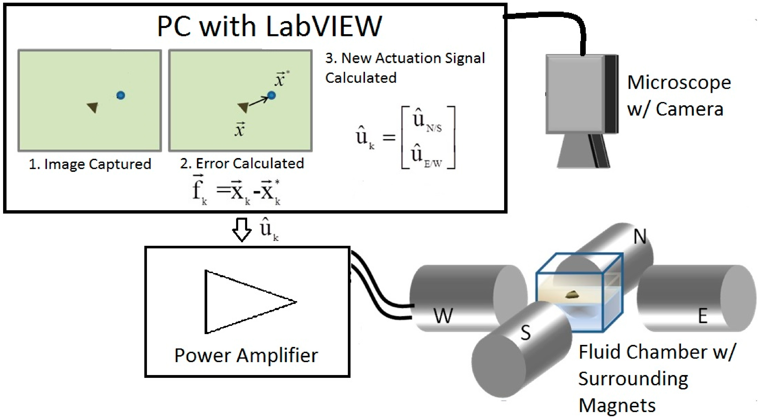
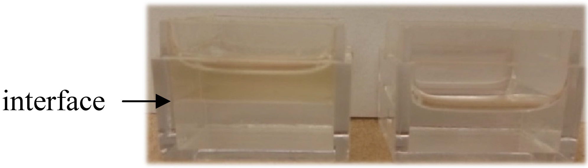
4.1. Experimental System

A microrobot system has been implemented comprised of an electroplated nickel slug suspended at the interface between two immiscible fluids, and an electromagnetic actuation system. The microrobot devices are 20 μm thick and fit within a 200 μm diameter circle and were fabricated through the MEMSCAP MetalMUMPS process (Crolles, France) [28]. A variety of device morphologies (developed for an earlier microrobot competition [29]) provide an opportunity to study the effects of different robot shapes (which possess different viscous drag characteristics), and are shown in Figure 3.
The microrobot operates at the interface between vegetable oil, and a solution consisting of sodium chloride and sodium bicarbonate dissolved in water, as shown in Figure 4.
Figure 3. Models of the different microrobot designs derived from the mask layout, rendered in MEMSPro. The designs are referred to as: (a) “S”, (b) bar, (c) “wedge”, and (d) “star”. Each device is approximately 200 μm in diameter.
Micromachines 05 00797 g003
Figure 4. On the left is the fluid chamber (20 × 20 × 15 mm) showing the fluid interface between oil (top layer) and a sodium chloride/sodium bicarbonate solution (bottom layer) that comprises the microrobot’s planar work surface. On the right is the concave meniscus that occurs without the oil layer.
Micromachines 05 00797 g004
The robots and fluid are in a 20 × 20 × 15 mm vial placed at the center of four cylindrical electromagnets arrayed along the four points of the compass. Each magnet is driven with a pulse of amplitude 11 V and frequency 100 Hz. The duty cycle of the control signal is varied from 0% to 50%. By varying the amplitude or duty cycle of square wave input voltages to each electromagnet, the varying magnetic field imposed on the microrobot imposes varying forces that propel the microrobot through its workspace.
The robots have no permanent magnetization. When placed in a magnetic field they develop an induced magnetization. If the field is non-uniform this leads to motion in the direction of increasing magnetic field strength. We utilize a simple actuation scheme with a magnet for each cardinal direction where only one magnet is actuated at a given time to pull the robot in the desired direction. Visual feedback is used to measure the position of the microrobot device. The vision system consists of a microscope and a 740 × 480 USB camera. System integration is achieved in LabVIEW environment with an 8 Hz vision update rate. Simple thresholding is used to distinguish the microrobot object from the background, and the centroid of the object is used as the robot position. The robustness of binarization is enhanced by backlighting the microrobot beneath the fluid.

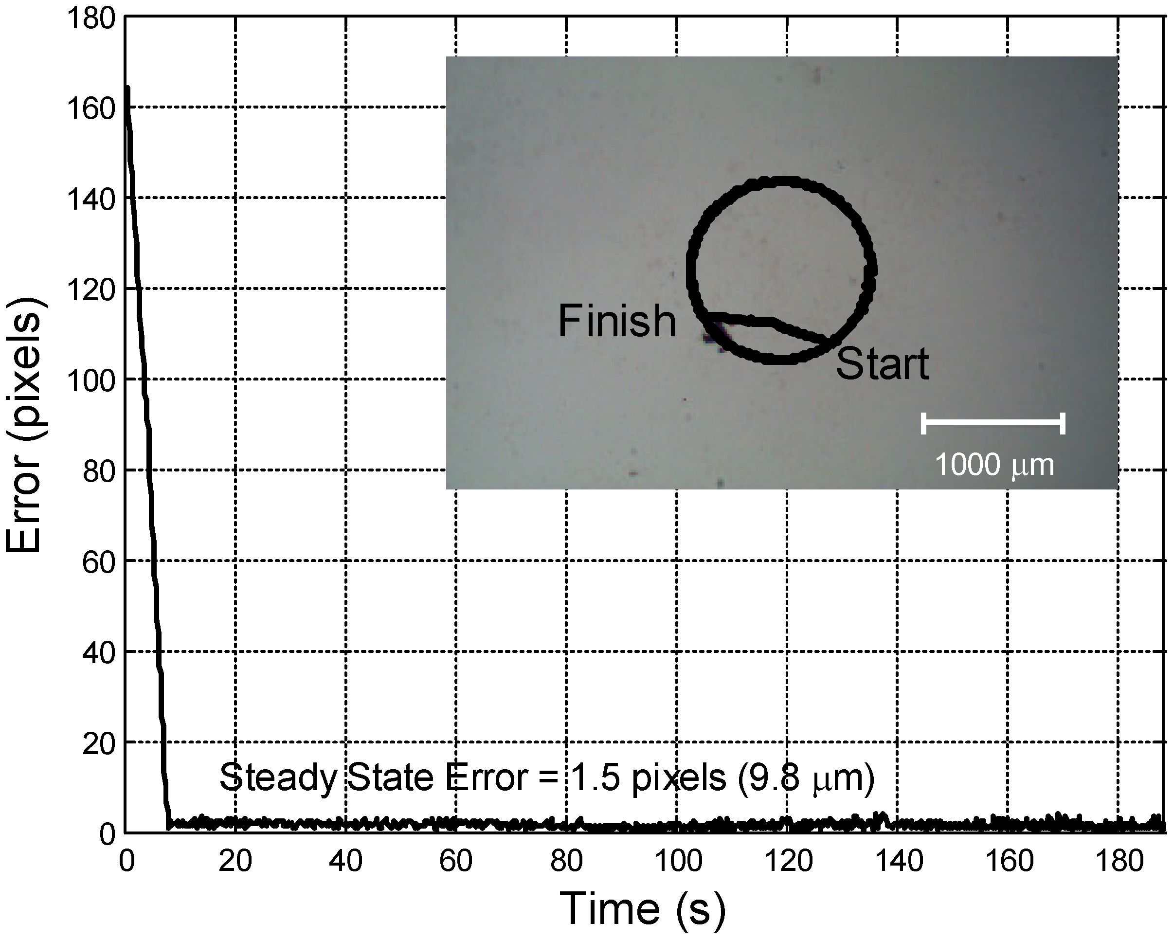
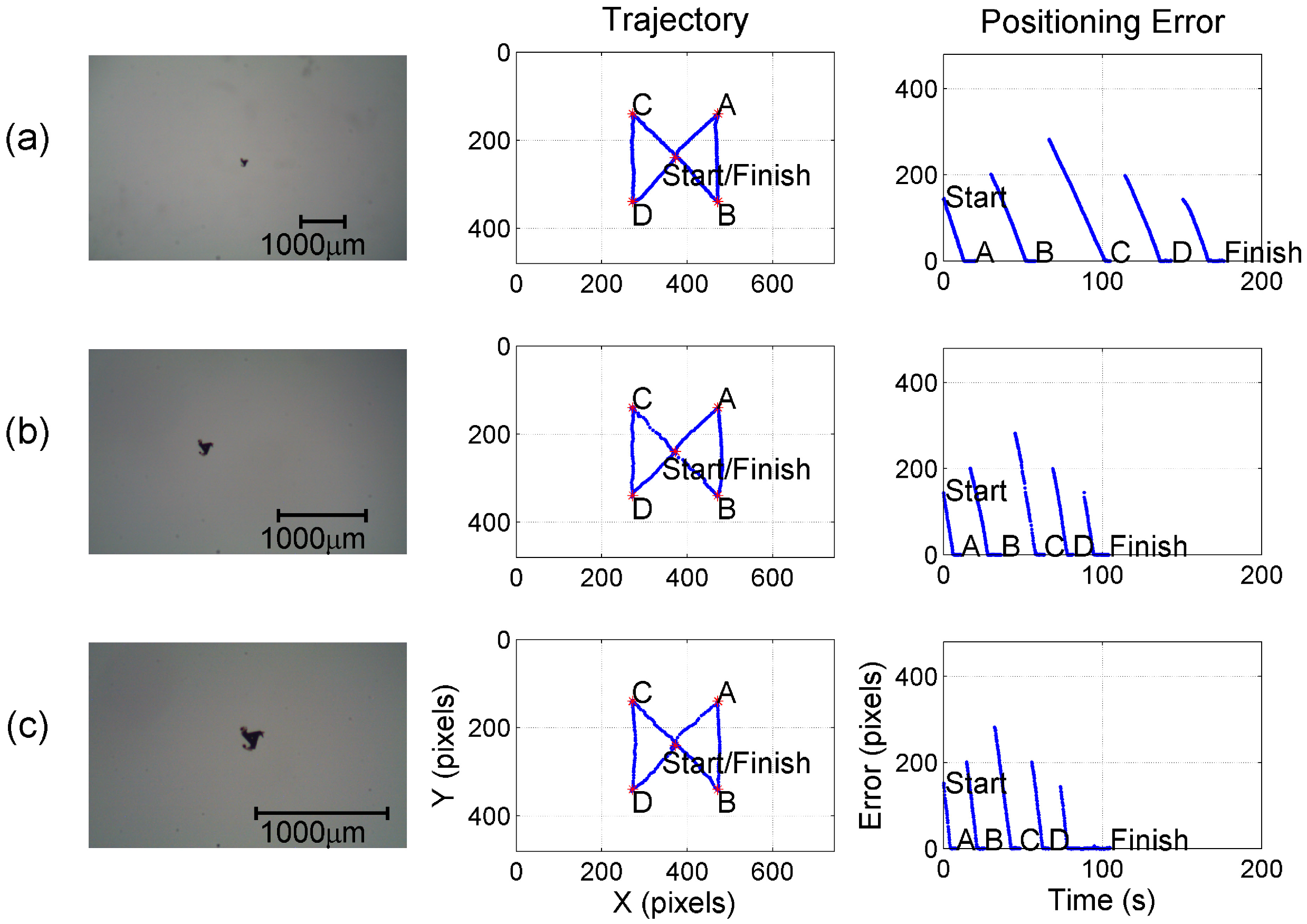
4.2. Stationary Target: Point to Point Motion

To demonstrate the robustness of the control a microrobot device is commanded a sequence of point-to-point motions throughout the field of view of system with the following variations:
  • Magnification
  • Electromagnet position and orientation
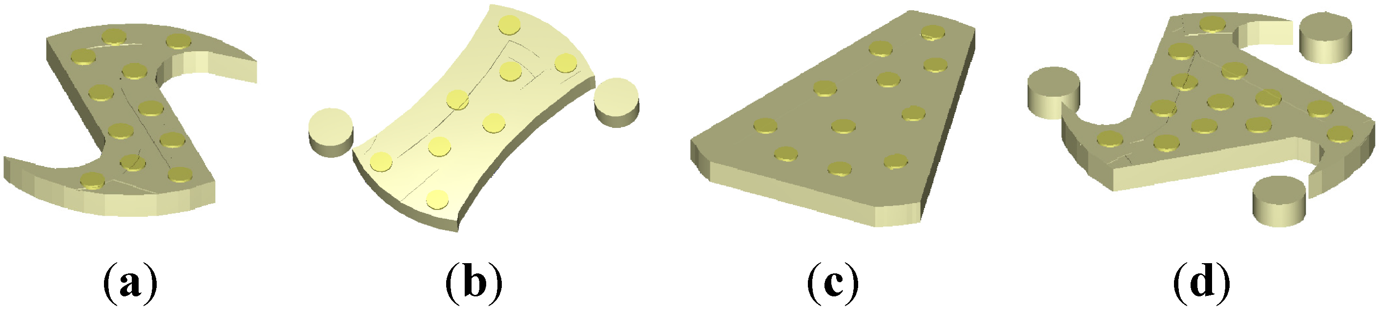
  • Microrobot device morphology
Figure 5, Figure 6 and Figure 7 show the variation, trajectory, and error (distance from robot to goal position) for each of these variations, respectively. The figures demonstrate convergent control for a wide variety of system configurations with no a priori knowledge, calibration, tuning, or careful fixturing of the components. For each experiment, the initial Jacobian matrix J0 and the covariance matrix P0 were set to the identity matrix and the recursive least squares algorithm was used to control the robots from one point to the next using λ = 0.99.
In Figure 5, results are shown demonstrating point-to-point motion throughout the field of view for three different magnifications {10×, 20×, and 30×}. The corresponding pixel resolutions are approximately 9.8, 6.5, and 3.25 μm/pixel, respectively. Starting in the center of the image, the microrobot devices are commanded to a sequence of points (denoted with A, B, C, and D). This self-intersecting quadrilateral path ensures that all four magnets are utilized for the robot motion and covers a large portion of the workspace. Note that the trajectories in the second column are plotted on axes equivalent to the image resolution shown in the first column.
Figure 5. Point-to-point control for three different magnifications {(a) 10×, (b) 20×, and (c) 30×} showing the image plane trajectory and the error between the goal position and the microrobot over time. The same algorithm and initial parameters were used in each case.
Micromachines 05 00797 g005
The same experiment is repeated for three different electromagnet configurations at 20× magnification as shown in Figure 6 demonstrating the adaptive ability of the controller to handle vastly different system configurations. If the controller were based on a system model (e.g., H or PID), these significant alterations to the system configuration would render the controller ineffectual. Rather, the only difference that is demonstrated is found in row (c) where a reduced speed in downward motion is observed. This is due to the weaker magnetic field affected by pulling one magnet away. The system is still convergent and achieves each goal position. Notice that rows (a) and (b) would require significantly different inputs from the electromagnet pairs for up and down motion as compared with row (b) in Figure 5 where up and down motion can be affected with inputs from the north or south magnets.
Figure 6. Trajectory and error for point-to-point motion. In row (a), the electromagnets were rotated approximately 45° counter-clockwise from the nominal compass-based orientation; row (b) demonstrates results for a in the opposite direction; and row (c) gives results when the south magnet was pulled away from the microrobot device several centimeters.
Micromachines 05 00797 g006
Figure 7. Point-to-point control of three different microrobot devices using the same algorithm and initial conditions: (a) “S”, (b) “bar” and (c) “wedge” shaped devices. These were performed at a 20× magnification and may be compared to the “star” device in Figure 5b. Noticeably, the wedge device moves the most quickly, but each microrobot device converges on the target points.
Micromachines 05 00797 g007
The experiments are repeated again at 20× for three more microrobot device morphologies. This is significant, because at this scale the different shapes will have different viscous drag coefficients. Indeed, this is indicated by the various speeds demonstrated in the positioning error plots; the rows (b) and (c) demonstrate significantly faster systems than row (a) or Figure 5b. A model-based controller would need to be calibrated to each device shape; however, the recursive least squares control is able to learn the system and servo each device to the goal positions. While the motion appears more erratic, it should be observed that the control method is designed to simply converge towards the static target points. The trajectory path is demonstrated in the following section.
All three figures repeatedly demonstrate convergent motion towards the target points under disparate conditions with no initialization or calibration.

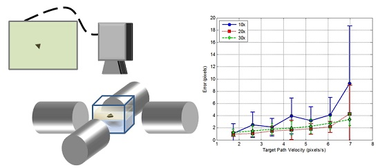
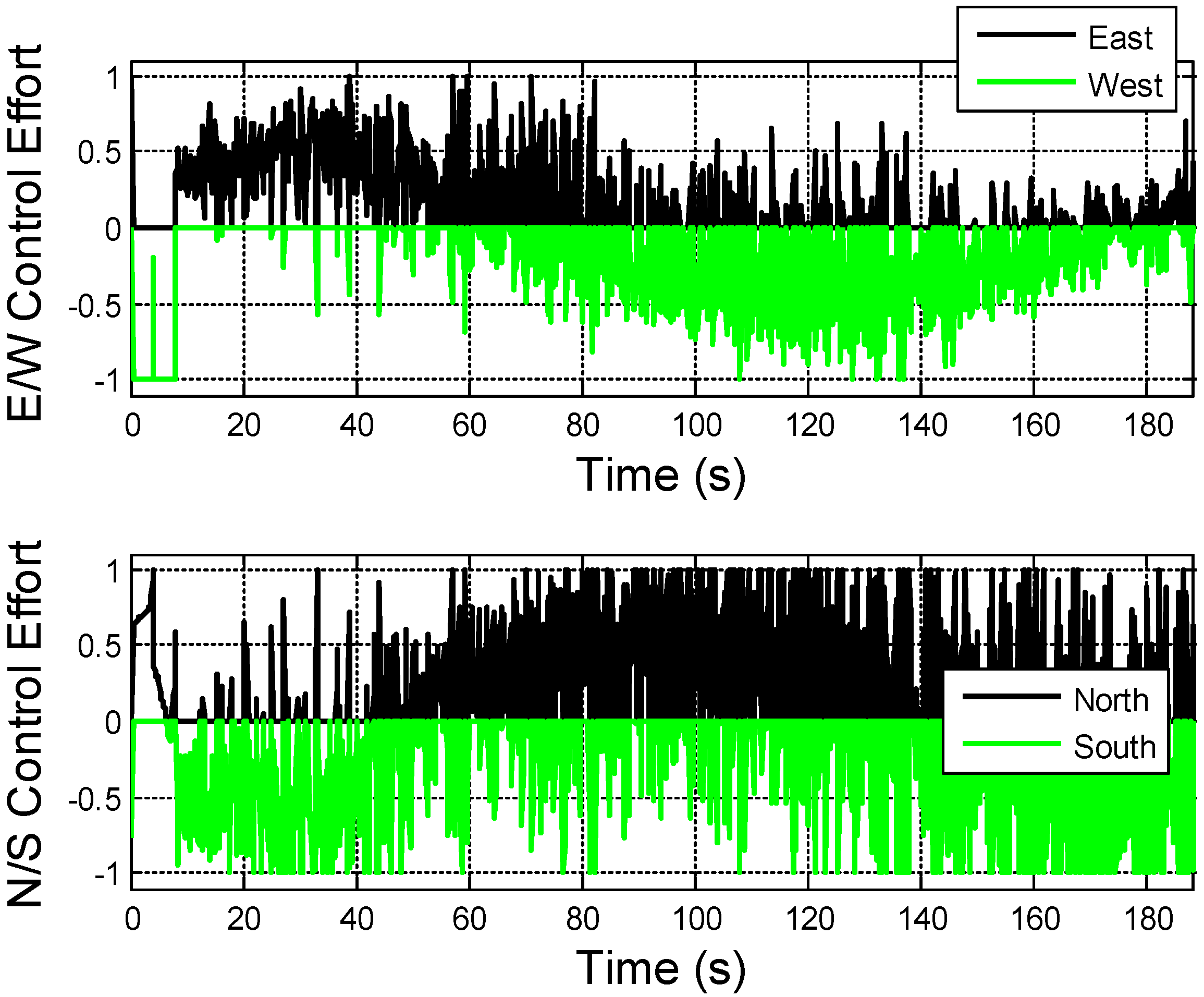
4.3. Moving Target: Circular Motion

The inclusion of the target velocity term x k * / t   h t term in the RLS algorithm given in Section 3 enables the controller to minimize the error even when the target is moving. To demonstrate this, a circular path is given as a desired motion. Again, results in this section demonstrate the ability to actuate a microrobot device with one algorithm (without calibration) while varying the following aspects of the system:
  • Magnification
  • Target speed
  • Electromagnet array orientation
  • Microrobot morphologies
As with the stationary experiments, the initial Jacobian matrix J0 and the covariance matrix P0 were arbitrarily set to the identity matrix and the RLS algorithm was used to control the robots from one point to the next using λ = 0.99.

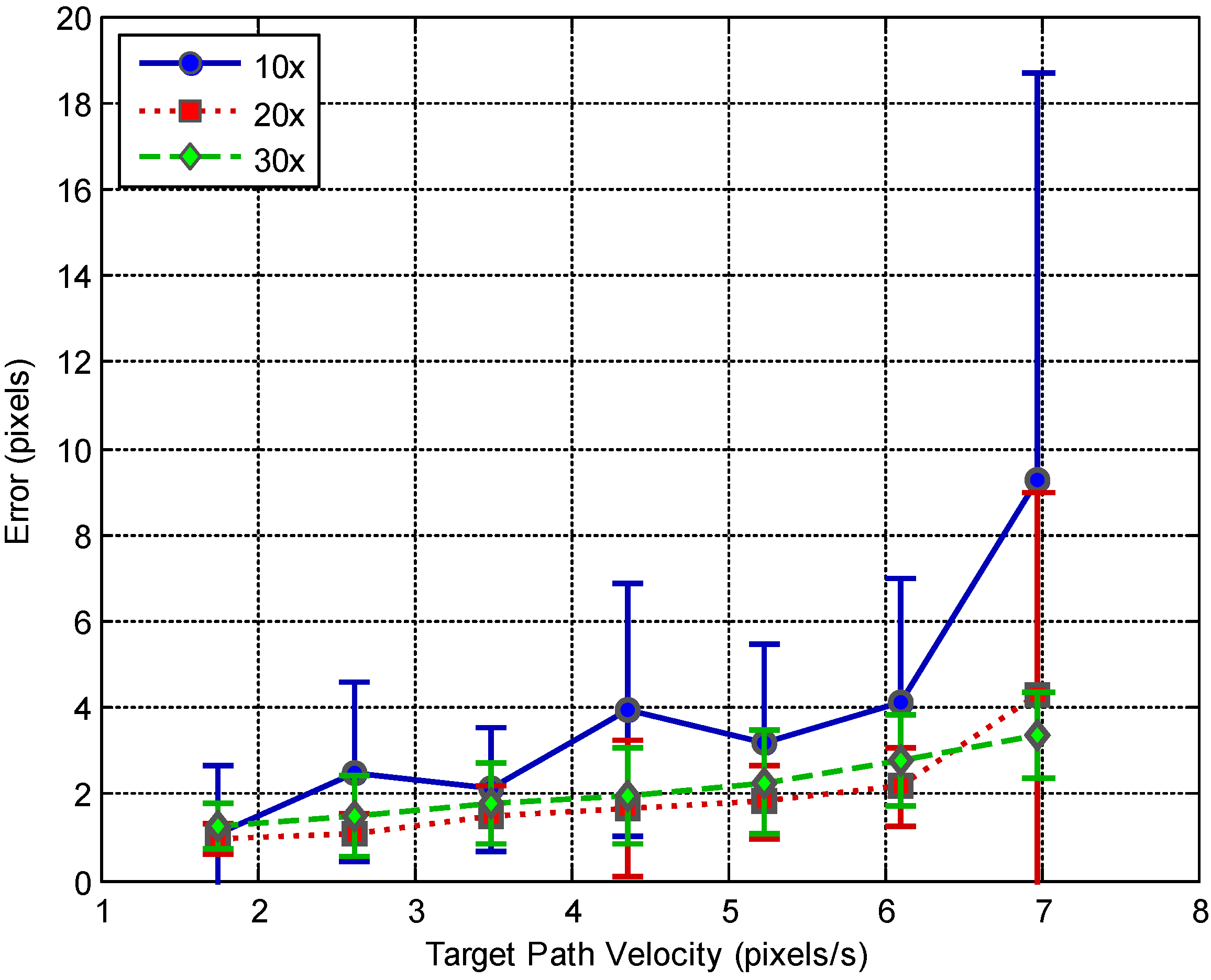
4.3.1. System Performance for Various Magnification and Target Speeds

Here, the steady state tracking error for a moving target prescribed as follows:
x * ( t ) = 100 [ cos ( ω t ) sin ( ω t ) ]  pixels
is studied for a range of angular velocities, at three different magnifications {10×, 20×, 30×}. As appropriate for an image-based visual servoing method, the error is presented in pixels at each magnification level.
First, Figure 8 demonstrates the path, tracking error, and control effort made during one such experiment with the magnification set at 20×. The target is moving as described in Equation (15) where ω = 0.035 rad/s which results in an average speed (tangential velocity) of 3.5 pixels/s or approximately 22.8 μm/s. The inset in Figure 8 records the path as the microrobot starts at the denoted location, servos towards the desired trajectory and continues around in a counter clockwise manner until it reaches the point where it initially met the desired path. The error between the microrobot and the desired path is shown demonstrating initial convergence and a steady state tracking error of 1.5 pixels.
The normalized control effort u ̂ k for the experiment depicted in Figure 8 is presented in Figure 9 with each subplot providing the scaled control signals sent to each electromagnet pair (where a scaled effort of 1 represents a 50% duty cycle signal sent to the electromagnet). This control effort varies a great deal as the controller seeks to make small moves keeping the microrobot on the desired path. The target velocity is such that the change in the goal position is on the order of the resolution of the position measurement and the signal is noise dominated. However, the underlying sinusoidal effort is observed with an expected 90° phase shift between the N/S and E/W electromagnet pairs.
Figure 8. Tracking error in pixels between actual robot position and desired path. The steady state error is 1.5 pixels, and the inset demonstrates the captured path of the robot.
Micromachines 05 00797 g008
Figure 9. Normalized control effort for the experiment given in Figure 8. The effort is normalized such that a 1 represents the maximum 50% duty cycle applied to a magnet. Positive values are applied to one magnet (E or N) of each magnet pair (N/S, E/W).
Micromachines 05 00797 g009
To more thoroughly investigate performance, the steady state tracking error is presented in Figure 10 for a series of experiments conducted at varying target speeds and system magnifications with error bars representing one standard deviation. The results convey both the limitations and strengths of the approach. Clearly the tracking error is greater for the 10× scenario. This makes sense in terms of system signal to noise ratios. At 10× magnification, the device is a smaller blob in the image which can result in more noise in the centroid calculation that is used to determine the position at each step. Furthermore, a given control signal results in a smaller motion (in pixels) than it would at a higher magnification. With greater system noise relative to observed motion, there is increased error in the tracking of the path.
Additionally, it is observed that there is increased tracking error as the target path velocity is increased. To a certain extent, this is to be expected and is similar to the results seen in [25], however the large errors seen at the highest speed for the 10× and 20× magnification are not a failure of the control system but rather due to the limitations of the electromagnets, which are not able to produce the required speeds for the microrobots at these settings. Inspection of the control effort for those two experiments shows saturation at the maximum allowed values.
Overall, Figure 10 demonstrates that when the target is moving at system achievable speeds, we demonstrate stable control for a 200 μm device following a moving target profile with average steady state errors ranging from 1.0 to 4.1 pixels in the image plane which translates to 4.1–40.5 μm in the workspace.
Figure 10. Average steady state tracking error (in pixels) with error bars indicated one standard deviation for a range of velocities and magnifications for a star microrobot following a circular path at three different magnifications (10×, 20×, and 30×). The pixel resolutions are approximately 9.8, 6.5, and 3.2 μm/pixel, respectively.
Micromachines 05 00797 g010

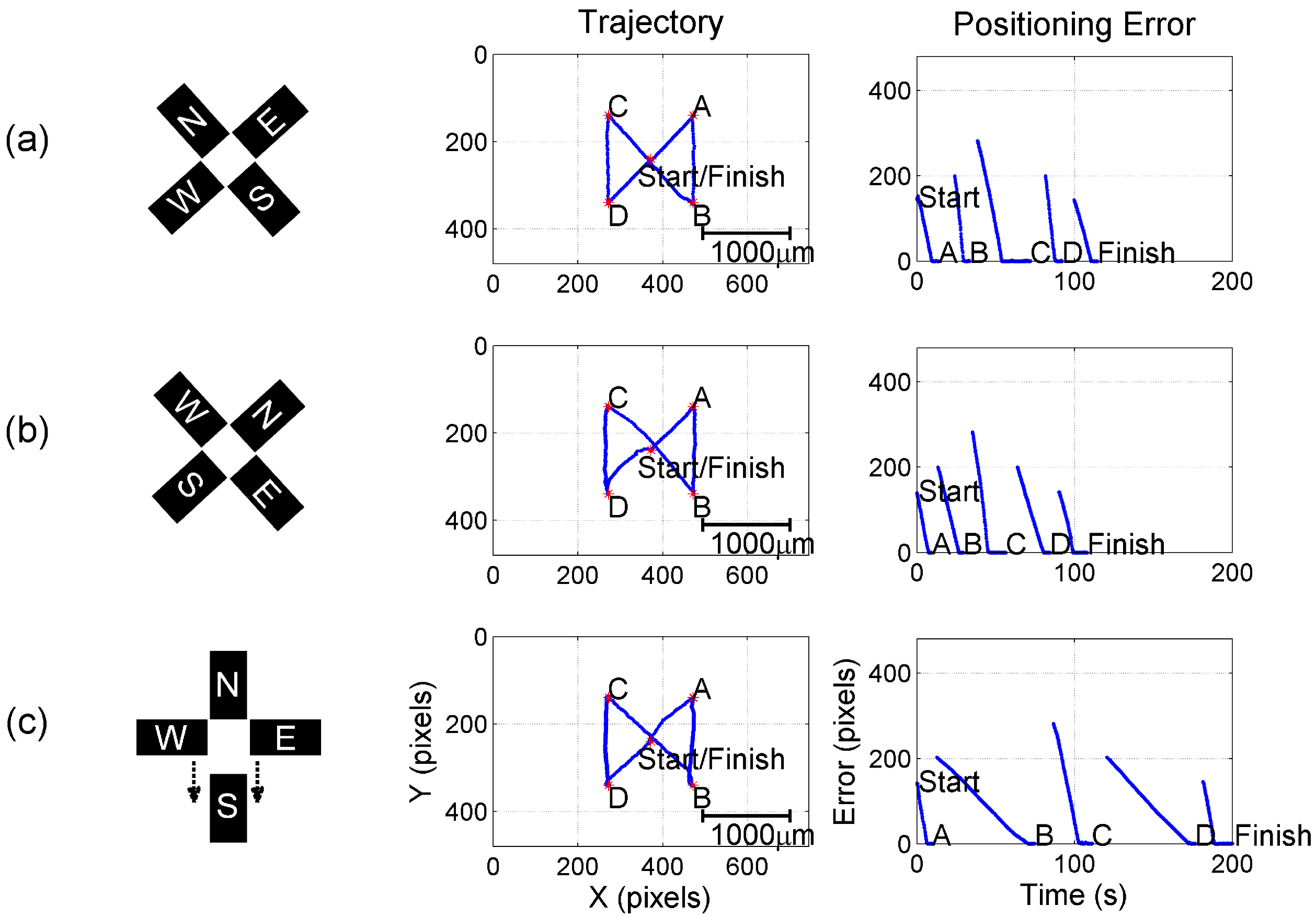
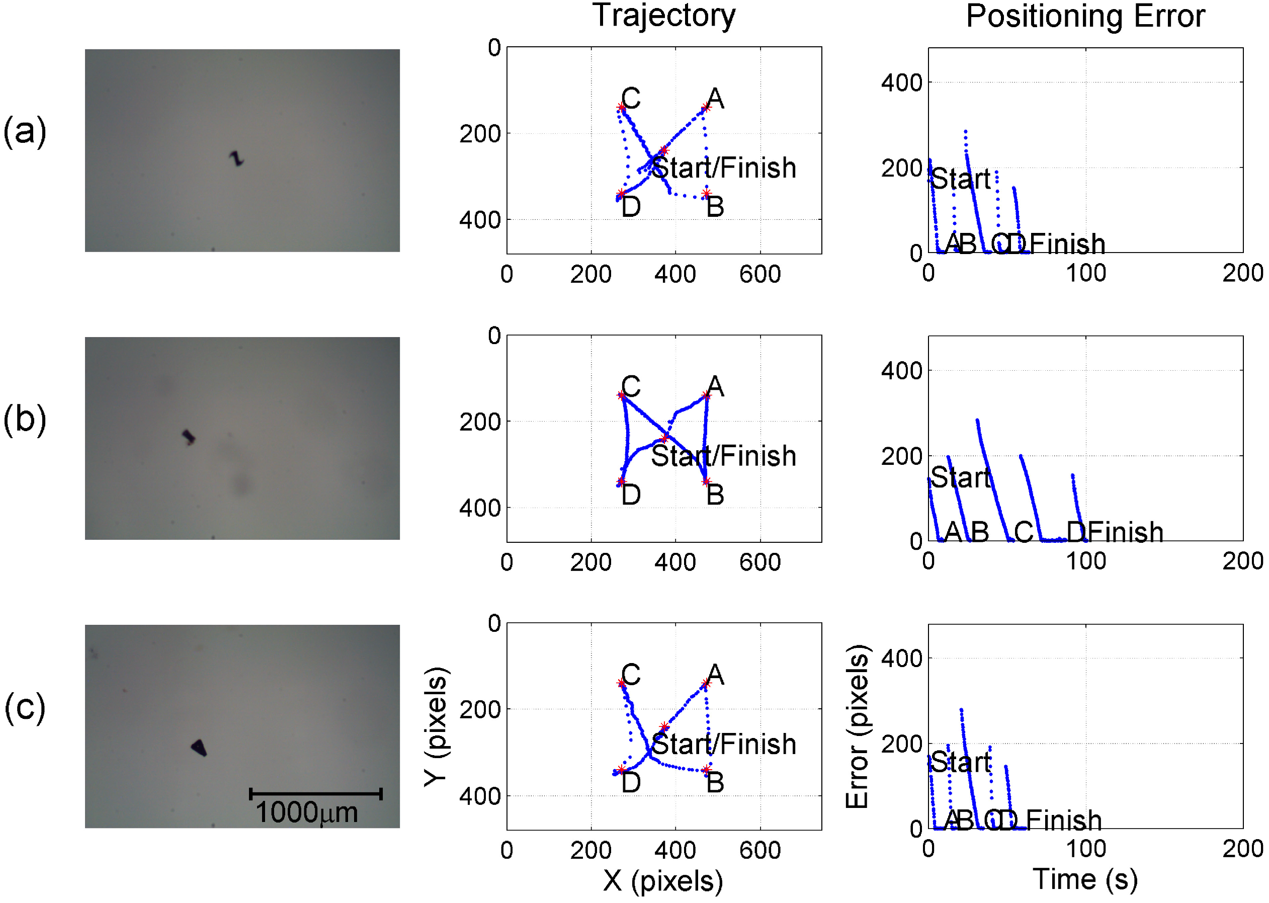
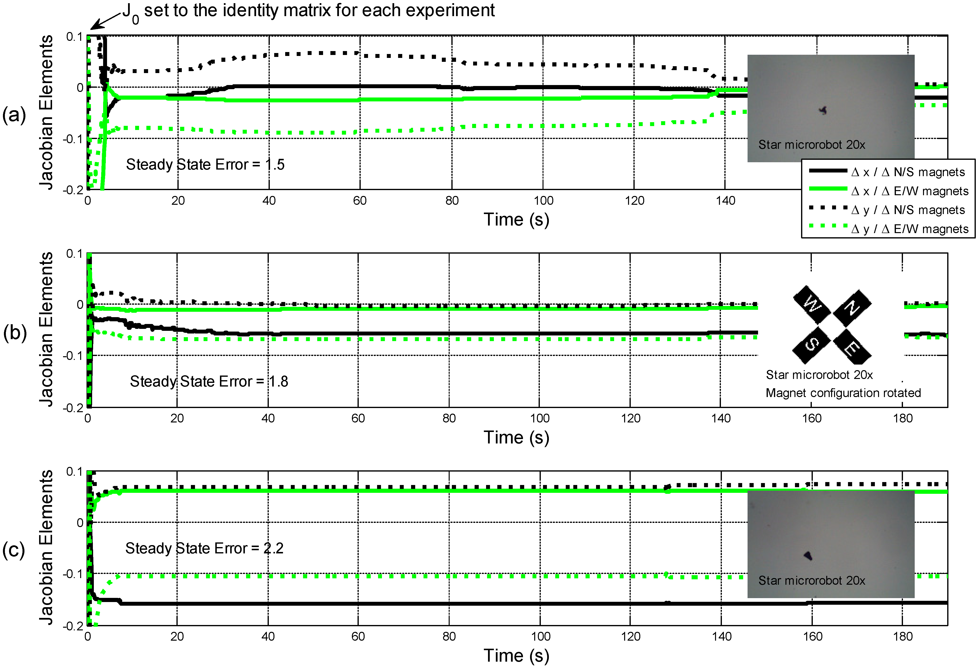
4.3.2. Tracking Performance for Various System Modifications

To demonstrate the versatility of the controller, the same moving target experiment is repeated for two significant system modifications using the same target path described in Equation (15). First, the magnetic array is rotated 45° (the target speed is set at 3.5 pixels/s and the magnification is set at 20×). While this is a simple coordinate frame rotation, it represents completely different system gains since a single magnet pair now induces motion in both the x and y direction of the image plane. In a second experiment, a different microrobot shape, one resembling wedge, is used. At this scale, changes in microrobot morphology can have significant effects on the viscous drag exerted on the device by the surrounding fluids.
If the controller were based on a system model (even a simple proportional controller), these alterations to the system configuration would render the controller ineffectual unless recalibrated. However, with the uncalibrated estimation, the system is still convergent and is able to follow the desired path. Figure 11 shows the Jacobian elements over time (J0 = I2) for the three different experiments. The values represent the ratio between changes in the robot’s position in the image (in both x and y) with respect to changes in the control effort sent to the two electromagnet pairs. In each experiment, the Jacobian values settle into very different numbers for steady state tracking (t > 5 s) because fundamental aspects of the system have changed, and the Jacobian estimation scheme is able to learn these changes.
Figure 11. Elements of the Jacobian estimation over time for three experiments: (a) a star microrobot with a nominal electromagnet configuration; (b) a rotated magnet configuration; and finally, (c) a wedge microrobot. In each case, the robot is given a circular path. Low steady state errors indicate effective tracking. Different system configurations result in different Jacobian values necessary for control. Online estimation eliminates the need for a priori calculation of these values.
Micromachines 05 00797 g011

5. Conclusions

This work has experimentally demonstrated an uncalibrated vision-based control method using recursive least squares for a magnetically actuated microrobot system working in a planar fluid environment. The uncalibrated nature of the controller was demonstrated by altering the magnification of the microscope, significantly rotating the electromagnet array, and by testing 200 μm robots with different morphologies. Despite all these changes, the uncalibrated image-based control method converges to stationary target points and demonstrates stable and consistent tracking results for moving target trajectories with average steady state path errors ranging from 1.0 to 4.1 pixels in the image plane (4.1–40.5 μm in the workspace). At a scale where accurate modeling of all system parameters can be difficult, the recursive least squares estimation and control method offers a great deal of flexibility for microrobot control with one algorithm capable of controlling a variety of system configurations.

Acknowledgments

The authors would like to acknowledge the work of Judy Raymond, Norm Tyson, Joe Bradshaw, Daphie Jobe, William Stanton, Erich Keyes, Ken Walsh, and Jerry Ballman, AshleyWessel, Peter Dausman, Louis Henry, Matthew Prevatt, Sean Johnson, Andrew Flora, Justin Aleshire, Kerri Bortz, Jeremy Gray, and Brett Morris.

Author Contributions

Jenelle Armstrong Piepmeier contributed to the writing of the manuscript and the design of the visual feedback control system. Samara Firebaugh contributed to the design and integration of the actuation system. Caitlin S. Olsen conducted a number of the experiments.

Conflicts of Interest

The authors declare no conflict of interest.

References

  1. Ishii, K.; Hu, W.I.; Ohta, A. Cooperative micromanipulation using optically controlled bubble microrobots. In Proceedings of IEEE International Conference on Robotics and Automation, Saint Paul, MN, USA, 14–18 May 2012; pp. 3443–3448.
  2. Hu, W.; Ishii, K.S.; Ohta, A.T. Micro-assembly using optically controlled bubble microrobots. Appl. Phys. Lett. 2011, 99. [Google Scholar] [CrossRef]
  3. Donald, B.R.; Levey, C.G.; McGray, C.D.; Paprotny, I.; Rus, D. An untethered, electrostatic, globally controllable mems micro-robot. Microelectromech. Syst. J. 2006, 15, 1–15. [Google Scholar] [CrossRef]
  4. Sul, O.J.; Falvo, M.R.; Taylor, R.M.; Washburn, S.; Superfine, R. Thermally actuated untethered impact-driven locomotive microdevices. Appl. Phys. Lett. 2008, 89. [Google Scholar] [CrossRef]
  5. Denisov, A.; Yeatman, E.M. Micromechanical actuators driven by ultrasonic power transfer. Microelectromech. Syst. J. 2014, 23, 750–759. [Google Scholar] [CrossRef]
  6. Bouchebout, S.; Bolopion, A.; Abrahamians, J.-O.; Régnier, S. An overview of multiple dof magnetic actuated micro-robots. J. Micro Nano Mechatron. 2012, 7, 97–113. [Google Scholar] [CrossRef]
  7. Jian, F.; Cho, S.K. Mini and micro propulsion for medical swimmers. Micromachines 2014, 5, 97–113. [Google Scholar] [CrossRef]
  8. Tamaz, S.; Gourdeau, R.; Mathieu, J.B.; Martel, S. Real-time mri-based control of a ferromagnetic core for endovascular navigation. IEEE Trans. Biomed. Eng. 2008, 55, 1854–1863. [Google Scholar] [CrossRef]
  9. Belharet, K.; Folio, D.; Ferreira, A. Control of a magnetic microrobot navigating in microfluidic arterial bifurcations through pulsatile and viscous flow. In Proceedings of IEEE/RSJ International Conference on Intelligent Robots and Systems (IROS), Vilamoura-Algarve, Portugal, 7–12 October 2012; pp. 2559–2564.
  10. Pawashe, C.; Floyd, S.; Sitti, M. Two-dimensional autonomous microparticle manipulation strategies for magnetic microrobots in fluidic environments. IEEE Trans. Robot. 2012, 28, 467–477. [Google Scholar] [CrossRef]
  11. Diller, E.; Floyd, S.; Pawashe, C.; Sitti, M. Control of multiple heterogeneous magnetic microrobots in two dimensions on nonspecialized surfaces. IEEE Trans. Robot. 2012, 28, 172–182. [Google Scholar] [CrossRef]
  12. Diller, E.; Giltinan, J.; Sitti, M. Independent control of multiple magnetic microrobots in three dimensions. Int. J. Robot. Res. 2013, 32, 614–631. [Google Scholar] [CrossRef]
  13. Floyd, S.; Pawashe, C.; Sitti, M. An untethered magnetically actuated micro-robot capable of motion on arbitrary surfaces. In Proceedings of IEEE International Conference on Robotics and Automation, Pasadena, CA, USA, 19–23 May 2008; pp. 419–424.
  14. Marino, H.; Bergeles, C.; Nelson, B.J. Robust electromagnetic control of microrobots under force and localization uncertainties. IEEE Trans. Autom. Sci. Eng. 2014, 11, 310–316. [Google Scholar] [CrossRef]
  15. Kummer, M.P.; Abbott, J.J.; Kratochvil, B.E.; Borer, R.; Sengul, A.; Nelson, B.J. Octomag: An electromagnetic system for 5-DoF wireless micromanipulation. IEEE Trans. Robot. 2010, 26, 1006–1017. [Google Scholar] [CrossRef]
  16. Bergeles, C.; Kratochvil, B.E.; Nelson, B.J. Visually servoing magnetic intraocular microdevices. IEEE Trans. Robot. 2012, 28, 798–809. [Google Scholar] [CrossRef]
  17. Ghanbari, A.; Chang, P.H.; Choi, H.; Nelson, B.J. Time delay estimation for control of microrobots under uncertainties. In Proceedings of 2013 IEEE/ASME International Conference on Advanced Intelligent Mechatronics (AIM), Wollongong, Australia, 9–12 July 2013; pp. 862–867.
  18. Keuning, J.D.; DeVriessy, J.; Abelmanny, L.; Misra, S. Image-based magnetic control of paramagnetic microparticles in water. In Proceedings of IEEE/RSJ International Conference on Intelligent Robots and Systems (IROS), San Francisco, CA, USA, 25–30 September 2011; pp. 421–426.
  19. Khalil, I.S.M.; Keuning, J.D.; Abelmann, L.; Misra, S. Wireless magnetic-based control of paramagnetic microparticles. In Proceedings of IEEE RAS/EMBS International Conference on Biomedical Robotics and Biomechatronics, Rome, Italy, 24–27 June 2012; pp. 460–466.
  20. Piepmeier, J.A.; Firebaugh, S.L. Visual servo control of electromagnetic actuation for a family of microrobot devices. In Proceedings of 2013 IEEE Workshop on Robot Vision (WORV), Clearwater Beach, FL, USA, 15–17 January 2013; pp. 209–214.
  21. Popa, D. Robust and reliable microtechnology research and education through the mobile microrobotics challenge [competitions]. IEEE Robot. Autom. Mag. 2014, 21, 8–12. [Google Scholar] [CrossRef]
  22. Purcell, E.M. Life at low reynolds number. Am. J. Phys. 1977, 45, 3–11. [Google Scholar] [CrossRef]
  23. Hosoda, K.; Asada, M. Versatile visual servoing without knowledge of true jacobian. In Proceedings of IEEE/RSJ International Conference on Intelligent Robots and Systems (IROS), Munich, Germany, 12–16 September 1994; pp. 186–193.
  24. Jagersand, M.; Fuentes, O.; Nelson, R. Experimental evaluation of uncalibrated visual servoing for precision manipulation. In Proceedings of IEEE International Robotics and Automation Conference, Albuquerque, NM, USA, 20–25 April 1997; pp. 2874–2880.
  25. Piepmeier, J.A.; McMurray, G.V.; Lipkin, H. Uncalibrated dynamic visual servoing. IEEE Trans. Robot. Autom. 2004, 20, 143–147. [Google Scholar] [CrossRef]
  26. Sakar, M.S.; Steager, E.B.; Cowley, A.; Kumar, V.; Pappas, G.J. Wireless manipulation of single cells using magnetic microtransporters. In Proceedings of IEEE International Robotics and Automation (ICRA) Conference, Shanghai, China, 9–13 May 2011; pp. 2668–2673.
  27. Eleftheriou, E.; Falconer, D.D. Tracking properties and steady-state performance of RLS adaptive filter algorithms. IEEE Trans. Acoust. Speech Signal Proc. 1986, 34, 1097–1110. [Google Scholar] [CrossRef]
  28. MetalMUMPs. Available online: http://www.memscap.com/products/mumps/metalmumps (accessed on 19 September 2014).
  29. Firebaugh, S.L.; Piepmeier, J.A. The robocup nanogram league: An opportunity for problem-based undergraduate education in microsystems. IEEE Trans. Educ. 2008, 51, 394–399. [Google Scholar] [CrossRef]

