2.1. Method: Ultrasonic Manipulation of Cells
Ultrasonic manipulation of suspended particles is based on the time-averaged acoustic radiation force. This forces origins from a non-linear effect in the acoustic pressure field and was first described by Lord Rayleigh [
19] and later nicely summarized in a review paper by Beyer [
20]. In 1962, a very useful theoretical model was presented by Gor’kov [
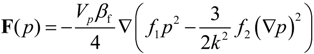
21]. This model is valid for arbitrary sound fields and a single, spherical particle with known material properties. Gor’kov’s generalized equation can be rewritten into the acoustic radiation force,
F, dependent on the sound field,
p and material properties [
22]:
with
here,
p is the acoustic pressure amplitude,
Vp is the volume of the particle,
β = 1/(
ρc2) is the compressibility (defined by the density,
ρ, and the sound speed,
c),
k=
ω/
c is the wave number, and
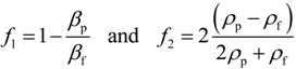
f1 and
f2 are the acoustic contrast factors defined by the compressibility
β and the density
ρ. The index “f” denotes “fluid” and the index “p” denotes “particle”. From the equation, we conclude that the radiation force drives suspended particles in a direction parallel with the gradient of the acoustic field and has a direction and magnitude defined by the contrast factors
f1 and
f2. The magnitude is also dependent on the particle volume,
Vp, and sound frequency (via
k =
ω/
c). Since steeper field gradients result in stronger forces, standing-wave fields are most often utilized. In a standing-wave field, the radiation force drives most suspended particles either to the pressure nodes or the pressure anti-nodes, depending on the signs of the contrast factors
f1 and
f2. In principle, particles stiffer than the suspension medium are driven to the pressure nodes (defined by the first term in Equation (1a)), while particles denser than the suspension medium are driven to the velocity antinodes (defined by the second term in Equation (1a)). In simple standing-wave fields (such as a one-dimensional field), the pressure nodes and the velocity antinodes are co-located. Although the standing-wave field in the multi-well plate is of more complex type, experimental observations confirm that the cells used in our work are driven to the positions of the numerically calculated pressure nodes [
16].
When several particles are driven to a pressure node, they tend to aggregate in tight clusters. In one-dimensional (1D) standing-wave fields, the clusters typically take the form of flat monolayers in the pressure nodal planes. The reason for this is the particle-particle interaction force, sometimes called the Bjerknes force [
23]. However, in 2D or 3D standing-wave fields, the cluster shapes are more complicated to predict or control [
24].
The theoretical model above (Equation (1)) is valid for spherical particles with well-known material properties (density and compressibility) suspended in an inviscid fluid. However, the method reviewed in this paper is designed for cell applications. Generally, cells have unknown material properties, or if known, their material properties have a wider distribution than for synthetic particles (e.g., polystyrene). In addition, the material properties of cells are also dependent on many external and internal factors. Altogether, this makes it difficult to predict the contrast factors
f1 and
f2 for cells. Nevertheless, attempts have been made to estimate the contrast factors and corresponding radiation forces acting on different cell types. For example, Barnkob
et al. [
25] used two types of particles (polystyrene and melamine resin) for calibrating the radiation forces from a known acoustic field, and used this data for measuring the contrast factors for two different cell types: White blood cells and DU145 prostate cancer cells. They concluded that the radiation force was about one order of magnitude smaller for these cells, relative polystyrene particles of equal size. A similar approach was carried out by Hartono
et al. [
26], who concluded that the radiation force was 1.5 times smaller for red blood cells, and between 2 and 4 times smaller for different types of cancer cells relative to the force on equally sized polystyrene. Furthermore, Mishra
et al. [
27] concluded from numerical modeling that for biological cells, the radiation force was less dependent on shape but more dependent on internal structures and inhomogeneity. For example, the force on a cell with nucleus was predicted to be approx. twice the force of a non-nucleated cell of similar size. In summary, we may expect the acoustic radiation force in a given acoustic field to be roughly a few times smaller for cells than for polystyrene particles of similar size, and that the corresponding trapping time is expected to be a few times longer.
2.2. Device: Ultrasonic Manipulation in a Multi-Well Micro-Plate
For the design of the multi-well microplate used for ultrasonic cell manipulation, the following criteria have been prioritized [
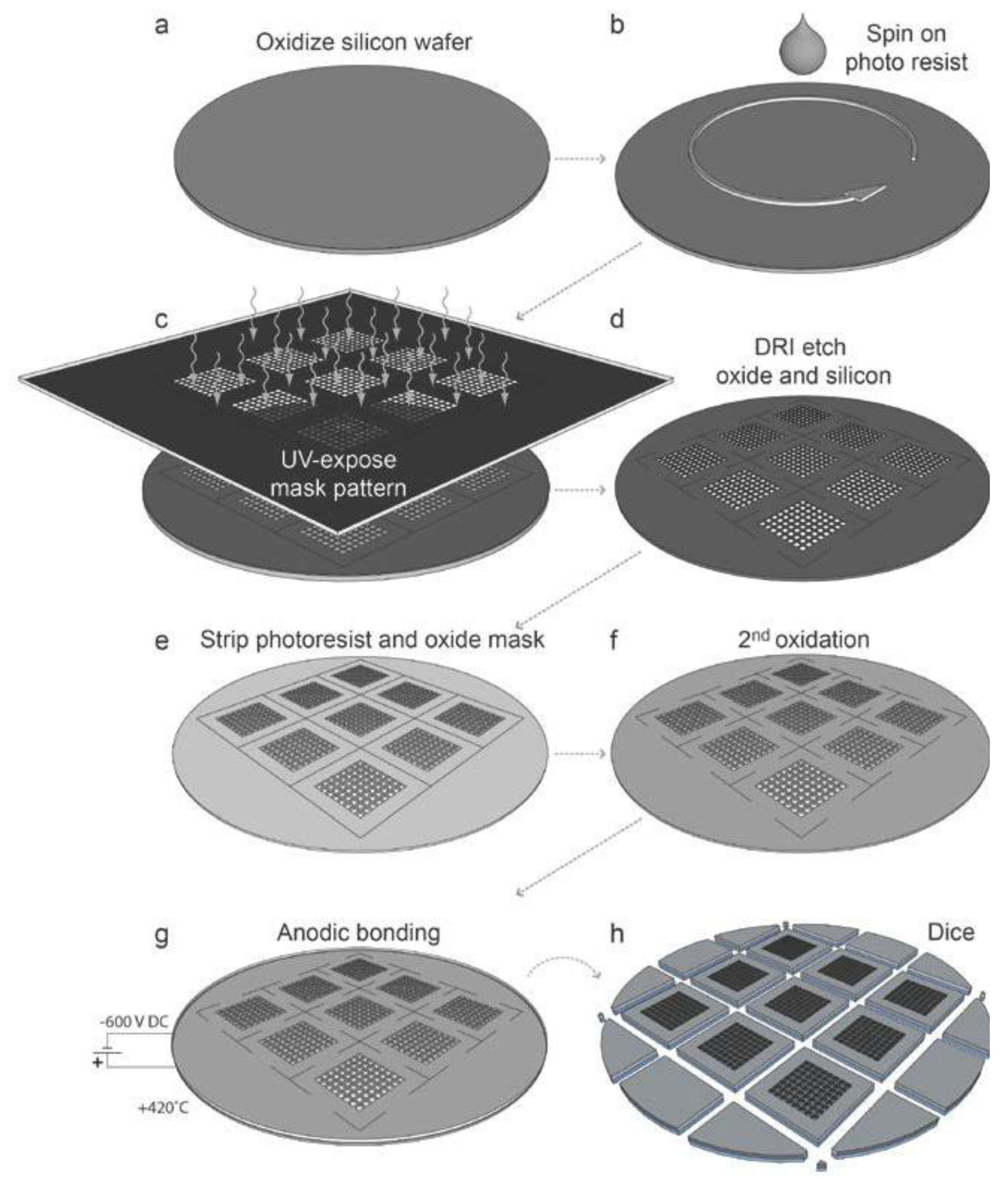
12]: The microplate should be compatible with high-resolution optical microscopy, and it should be biocompatible allowing long-term cellular assays. In addition, it should also be easy to use by a non-technically skilled operator. An illustration of the microplate fabrication process is shown in
Figure 1. A complete description of the fabrication process is given in Ref. [
12]. In summary, silicon wafers with diameter 100 mm and thickness 300 µm (
Figure 1a) were used for processing of nine individual microplates per wafer, where each final microplate is 22 × 22 mm
2 (
Figure 1h). Each microplate has 10 × 10 wells, where each well is 300 µm deep and with horizontal cross section 300 × 300 µm
2, or 350 × 350 µm
2, and with 100 µm wall thickness between individual wells. After spinning photo resist on the silicon wafer (
Figure 1b) and defining the well geometry by lithography (
Figure 1c), the wells were etched through the 300 µm silicon layer by deep reactive-ion etching (DRIE) (
Figure 1d). Care was taken to optimize the process so that the wells had a constant cross section through the depth of the silicon layer. This was confirmed by scanning electron microscopy (SEM) after the etching process and with a silicon layer that was diced across the wells [
12]. Following the deep-etching of the wells and stripping of the photo resist and oxide mask (
Figure 1e), the silicon wafers were furnace wet-oxidized to a surface oxide thickness of approx. 200 nm (
Figure 1f). This important step was performed for improving the biocompatibility [
12], and also for enabling cleaning and re-usage of the microplates. Finally, a 175 µm thick borosilicate glass layer was anodically bonded to each processed silicon layer (
Figure 1g), and the silicon-glass stack was diced into square-shaped microplates (
Figure 1h).
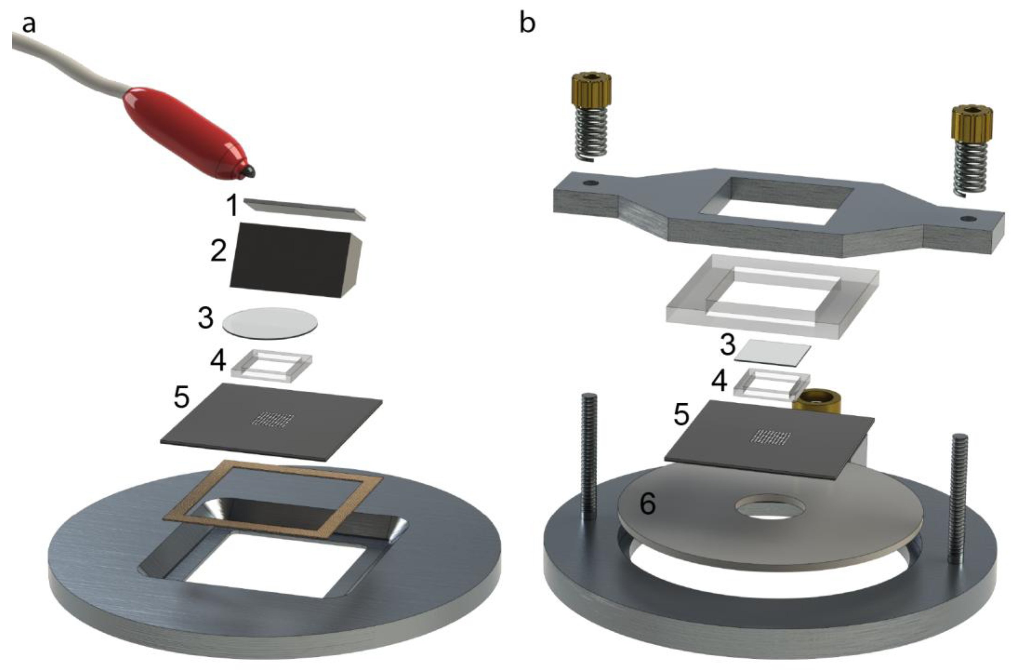
Two different designs have been used for the ultrasonic actuation system for the microplates. The original design [
16,
18] used a wedge-transducer [
22,
28] (
Figure 2a). In the upgraded version of the ultrasonic actuation system, the wedge transducer was replaced by a ring transducer, which was fully integrated into the microplate holder [
17] (
Figure 2b). This device is more robust and simple to use, but requires higher driving voltages. The wedge-transducer device (
Figure 2a) consists of an ultrasonic transducer made by a piezoceramic plate (1) and a titanium wedge (2). The transducer is positioned on top of the multi-well microplate (5), and it is reversibly glued with a thin layer of water-soluble adhesive gel. The cell suspension sample is pipetted from above over the wells and stored within a rectangular frame made in PDMS (4), which can be closed by a glass cover slip (3) to minimize evaporation. The other device, the ring-transducer chip (
Figure 2b), has the same general function including parts (3)–(5), but here the ultrasonic coupling is accomplished from below via a larger ring-shape piezoceramic plate (6). This design is more robust and reliable since it is not dependent on how the transducer is positioned relative to the chip. Furthermore, it is also more temperature-stable when driven at higher voltages (>20 Vpp) and therefore more suitable for applications requiring higher radiation forces, faster response times and long assay times (up to several days). Both designs shown in
Figure 2a,b are relatively broadband, which is useful for the employed ultrasonic actuation method described below.
Figure 1.
Schematic outline of the silicon-glass microplate fabrication process. (
a) Oxidized silicon wafer, 100 mm in diameter, 300 µm thick; (
b) Spin coating of wafer with positive photoresist; (
c) Masked UV-exposure of photoresist layer; (
d) Plasma etching of the oxidized silicon wafer; (
e) Removal of photoresist and oxide mask; (
f) Oxidation of the wafer after the strip of the photoresist and oxide mask; (
g) The anodic bonding of the 175 µm thick glass bottom to the silicon “grid”; (
h) Dicing to individual chips, 9 per wafer, where each final chip is 22 × 22 mm
2. Based on a figure in Ref. [
12].
Figure 2.
The two different designs of ultrasonic actuation system used for the multi-well microplate: The wedge-transducer device [
18] (
a) and the ring-transducer device [
17] (
b). (1) Piezoceramic plate; (2) Titanium wedge; (3) Glass lid; (4) PDMS frame; (5) Multi-well microplate; (6) Ring-shaped piezoceramic plate.
The purpose of the ultrasonic actuation in the multi-well microplate is to create an acoustic resonance in each well, so that suspended particles or cells are aggregated and positioned by the acoustic radiation force described by Equation (1). The trapping position is in most cases the pressure node of the standing wave formed in the fluid cavity (
i.e., the well) by the acoustic resonance. In a two-dimensional rectangular cavity with dimensions
Lx and
Ly, the acoustic pressure,
p, is described by [
29]:
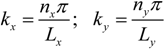
where
kx and
ky are the wavenumbers for each horizontal direction (
x and
y) in the cavity, and
nx,
ny= 0, 1, 2, 3, …, are the numbers of half wavelengths along the
x- and
y-directions, respectively. Note that in Equation (2), we have neglected any (vertical)
z-dependence of the pressure. In practice, this is valid for three-dimensional cavities having short
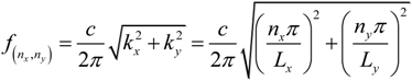
Lz-dimensions (relative the acoustic wavelength). Given an acoustic resonance in the fluid cavity described by Equation (2), the resonance frequency of mode (
nx,
ny) is [
29]:
where
c is the sound velocity in the fluid. If the purpose is to trap the particles in the center of each well, one should use the lowest possible resonance mode. The wells used in our multi-well microplate have square-shaped horizontal cross-sections (
cf. Figure 1,
Figure 3 and
Figure 4). For a square-shaped cavity (
Lx=
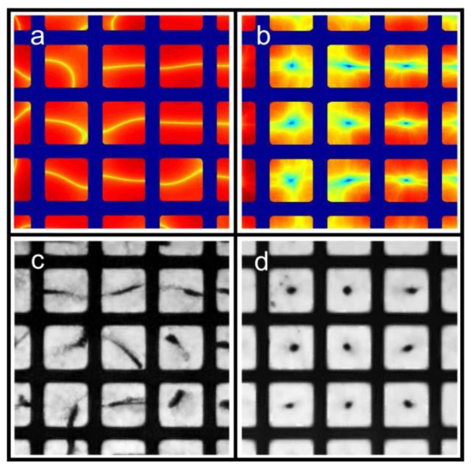
Ly), the lowest possible mode is either the (1,0)-mode or the (0,1)-mode. According to Equation (3), these two modes have identical frequencies, and it is therefore not clear how the pressure field can be described at this frequency. However, due to differences in boundary conditions and properties/shapes of the supporting structures around the wells, the two modes are often slightly degenerated. Thus, for a given excitation frequency, only one of the two modes exists. In our multi-well microplate, where a complex acoustic interaction between all 100 wells occurs, the result is a pressure field inside each well having a node oriented as shown in the simulated pressure field in
Figure 3a (and described more thoroughly in Ref. [
16]). As seen from the simulation, the node of the half-wave resonance in each well is not a pure (1,0)- or (0,1)-mode, but rather something in between. If the excitation frequency is slightly changed, the node orientation changes (primarily it rotates). For this reason, a simple method for generating point-shaped pressure nodes in the center of each well is to quickly average a set of such single-frequency resonances. We have realized this by cycling linear frequency sweeps around the nominal (1,0)- or (0,1)-resonance frequency. The simulation result of this frequency modulation scheme is shown in
Figure 3b. The simulated acoustic resonances in
Figure 3a,b are experimentally confirmed using the wedge-transducer device in
Figure 3c,d, respectively. Here, the pressure field is visualized by the shapes and positions of 5 µm polyamide particle aggregates driven to the pressure nodes by the acoustic radiation force. Experimentally, frequency modulation actuation is realized by sawtooth-modulation with a center frequency corresponding to the (1,0) or (0,1) resonance (which is around 2.5 MHz for a 300 × 300 µm
2 well) and a typical bandwidth of 100 kHz and a cycling rate of 1 kHz. This modulation function is very simple to implement since it is a built-in function in most signal generators. The modulation bandwidth is difficult to predict theoretically and needs instead to be optimized experimentally for each microplate device. The cycling rate is typically chosen as a rate being above the threshold for aggregate movement (
i.e., time for reconfiguration of the aggregate between different single- frequency resonances within the sweep). We have concluded that a rate of 1 kHz is well above this threshold. Finally, a similar experimental verification for the ring-transducer device is shown in
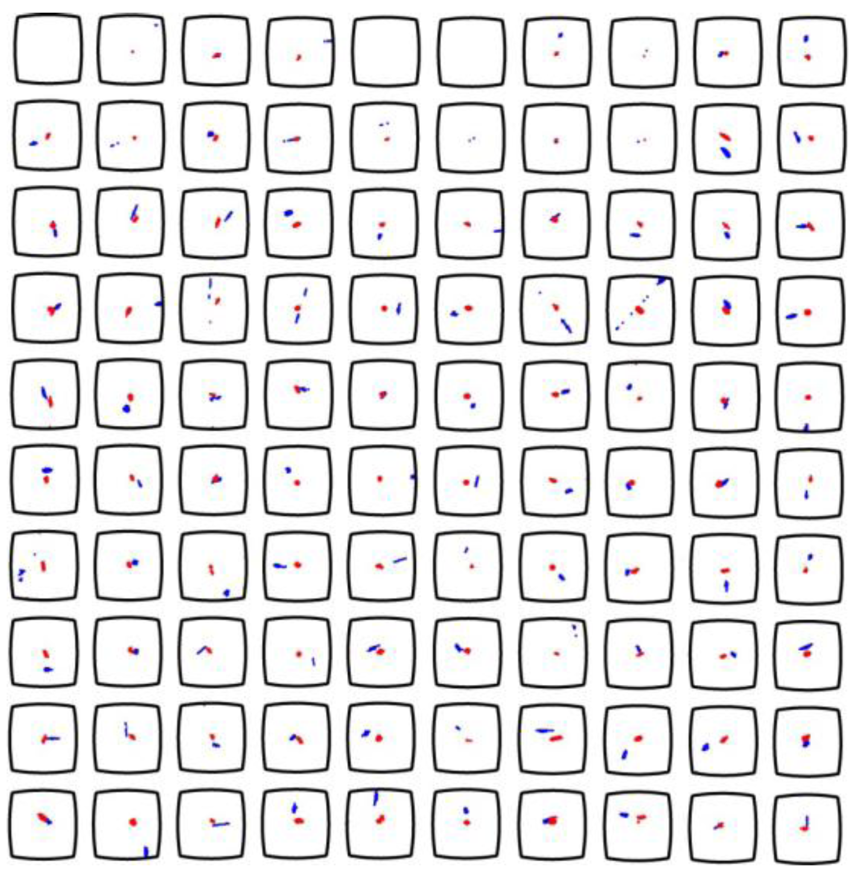
Figure 4. Here, we used a microplate with well size 350 × 350 µm
2 actuated with center frequency 2.30 MHz and modulation bandwidth of 200 kHz. When using a lower concentration of 10 µm particles, it is clear from the experiments that particle trapping and aggregation work for both single-frequency actuation (blue aggregates) and frequency-modulation actuation (red aggregates). However, the accurate positioning of aggregates in the center of each well can only be accomplished by frequency-modulation actuation. In addition, frequency modulation also provides more compact aggregates [
17].
A limiting factor for the trapping performance in any acoustophoretic device is acoustic streaming [
30]. In the multi-well microplate, acoustic streaming causes the trapped particles or cells to be flushed away upwards if very high actuation voltages are used (approx. 100 Vpp or more) [
17]. One reason for this streaming is that it is not an accurate approximation to model the wells in the microplate as 2D cavities (
cf. Equations (2) and (3)). Thus, Equations (2) and (3) are useful for qualitative understanding of how resonances are built up in the system and for predicting trapping positions of cells, but for accurate quantitative modeling including acoustic streaming, a 3D model is needed. This is a challenge for future work. Still, it should be mentioned that the frequency-modulation methods tends to suppress acoustic streaming when comparing with single-frequency actuation [
30,
31]. Thus, for moderate actuation voltages using the frequency modulation method, acoustic streaming is not causing any problem for the trapping efficiency and trapping stability over time.
Figure 3.
Comparison between modeling (
a,
b) and experiments (
c,
d) for the wedge-transducer device. Simulation of the time-averaged pressure squared (
p2) for single-frequency actuation at 2.60 MHz (
a) and for the average of 50 single frequencies between 2.55 and 2.65 MHz (
b). Both plots are normalized individually and shown in logarithmic scale. The predicted trapping locations (
i.e., the minima of
p2) are indicated in yellow (in
a) and in dark blue (in
b). Experimental confirmation of the simulations using 5 µm particles at single-frequency actuation (
c) and with frequency-modulated actuation (
d) using the same frequency intervals as (
a) and (
b). Scale bar is indicated by the wells (300 µm wide squares).The figure is reproduced from Ref. [
16] with permission from RSC.
Figure 4.
Detailed experimental evaluation of the trapping and positioning performance of 10 µm particles in the ring-transducer device. Scale bar is indicated by the wells (350 µm wide squares with slightly rounded walls). The actuation frequency is 2.30 MHz (single-frequency, blue aggregates) and 2.30 ± 50 kHz at the modulation rate 1 kHz (frequency-modulation, red aggregates). The figure is based on results presented in Ref. [
17].
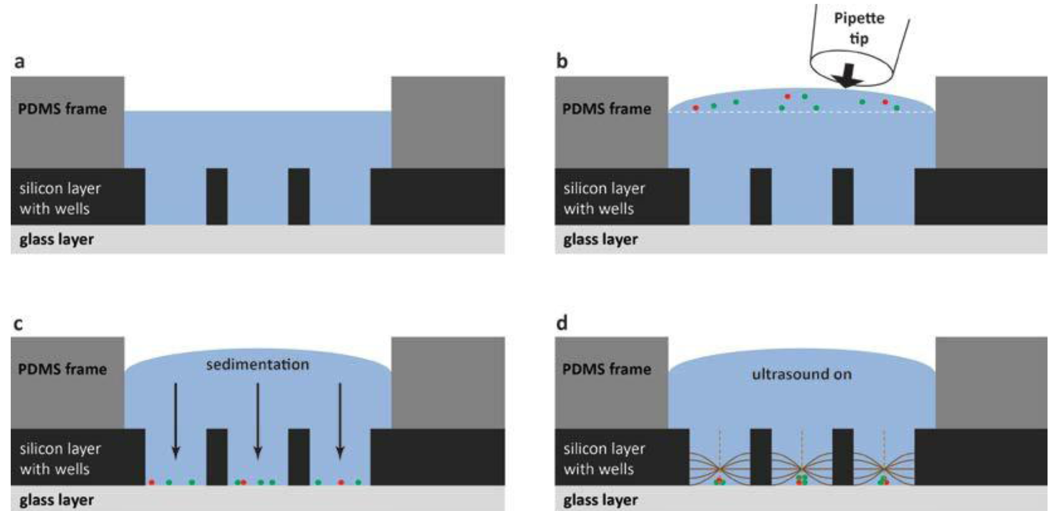
For the practical handling of the device with a cell suspension sample, the method is summarized in
Figure 5. The fluid reservoir within the PDMS frame shown in
Figure 5a has the purpose of providing a controlled environment of temperature- and CO
2-regulated cell medium. The cell medium volume (50 µL) needs to be large enough for enabling cell culturing over long terms (hours to days) and also for the practical handling (
i.e., enough to avoid sample evaporation). To this primed volume of cell medium, a small aliquot of cell suspension is pipetted from above (see
Figure 5b) before closing the device with the glass lid (
cf. item #3 in
Figure 2). The seeding of cells into the wells is based on gravitational settlement (see
Figure 5c). The strength of this method, besides simplicity, is the ability to study different numbers of cells per well interacting. Thus, the average number of cells per well is controlled by the cell concentration in the added drop (
cf. Figure 5b), and the seeding principle causes a stochastical distribution around this average. Finally, when ultrasound is applied with the frequency-modulation method presented in
Figure 3, the cells are aggregated and positioned in the center of each well where they can be monitored over time by high-resolution fluorescence microscopy. If confocal microscopy is used, it is a benefit to know the exact locations of the 100 cell aggregates. Since confocal microscopy is a relatively slow method, only the small area where the cells are located needs to be scanned, instead of the whole microplate.
Figure 5.
Schematic illustration (not to scale) of the different steps of the cell handling method. For simplicity, only three out of a hundred wells are shown (vertical cross-section view), and only the PDMS frame and the multi-well microplate (item #4 and #5 in
Figure 2). (
a) The microplate is first primed with cell medium shown in blue; (
b) The cell suspension is added as a small drop from a pipette tip; (
c) Cells sediment by gravity down into the wells. The average number of cells per well is controlled by the cell concentration in the added drop in (
b). In this example, there is on average 1 red cell and 2.33 green cells per well; (
d) When ultrasound is turned on according to the procedure described in
Figure 3, cells are trapped, aggregated and centrally positioned in each well.
2.3. Quantifying Acoustic Energy Density, Acoustic Pressure Amplitude, Acoustic Radiation Forces and Acoustic Streaming
In order to fully characterize the device, it is important to be able to measure the properties of the acoustic field including the acoustic radiation forces and acoustic streaming acting on the particles, cells and the fluid, respectively. In a resonant acoustic field, there is no clear propagation direction of the wave. For that reason, acoustic energy density is a commonly used measure. This energy density can be translated into, e.g., acoustic pressure amplitude or acoustic radiation force (
cf. Ref. [
17]). Thus, knowing these acoustic field properties is important for estimating the trapping efficiency of cells, but also for estimating the risk of having cavitation in the sample (see
Section 3). It is very difficult to measure the acoustic field properties by direct methods in an acoustofluidic device. However, there are different indirect methods available. Here, we will present three different methods used in our lab: Light intensity, particle tracking and particle image velocimetry (PIV). The methods are based on translating a measured property (i.e., light intensity, particle position or particle velocity) into acoustic energy density or acoustic pressure. All methods are based on one-dimensional (1D) geometries, but can be used for 2D geometries for order-of-magnitude estimations of the energy, pressure and forces.
The first method, light intensity, has been developed in collaboration with Rune Barnkob and Henrik Bruus (Denmark Technical University, Copenhagen, Denmark) [
28,
32]. This method is specifically designed for acoustofluidic chips that are optically transparent and compatible with standard bright-field microscopy [
6]. One strength of the light intensity method is that the chips do not need to be compatible with high-resolution microscopy. For example, individual particles do not need to be resolved, and relatively high particle concentrations (up to 10
9 beads/mL) can be used. In brief, the method is based on measuring the total transmitted light intensity passing through a certain part of a microchannel or a microchamber during the focusing process of suspended particles. When particles are focused and trapped in the pressure node, the fluid cavity gradually becomes more transparent for light. A detailed description of the method is found in Ref. [
32], but here it is sufficient to show an example of what the method can be used for. In
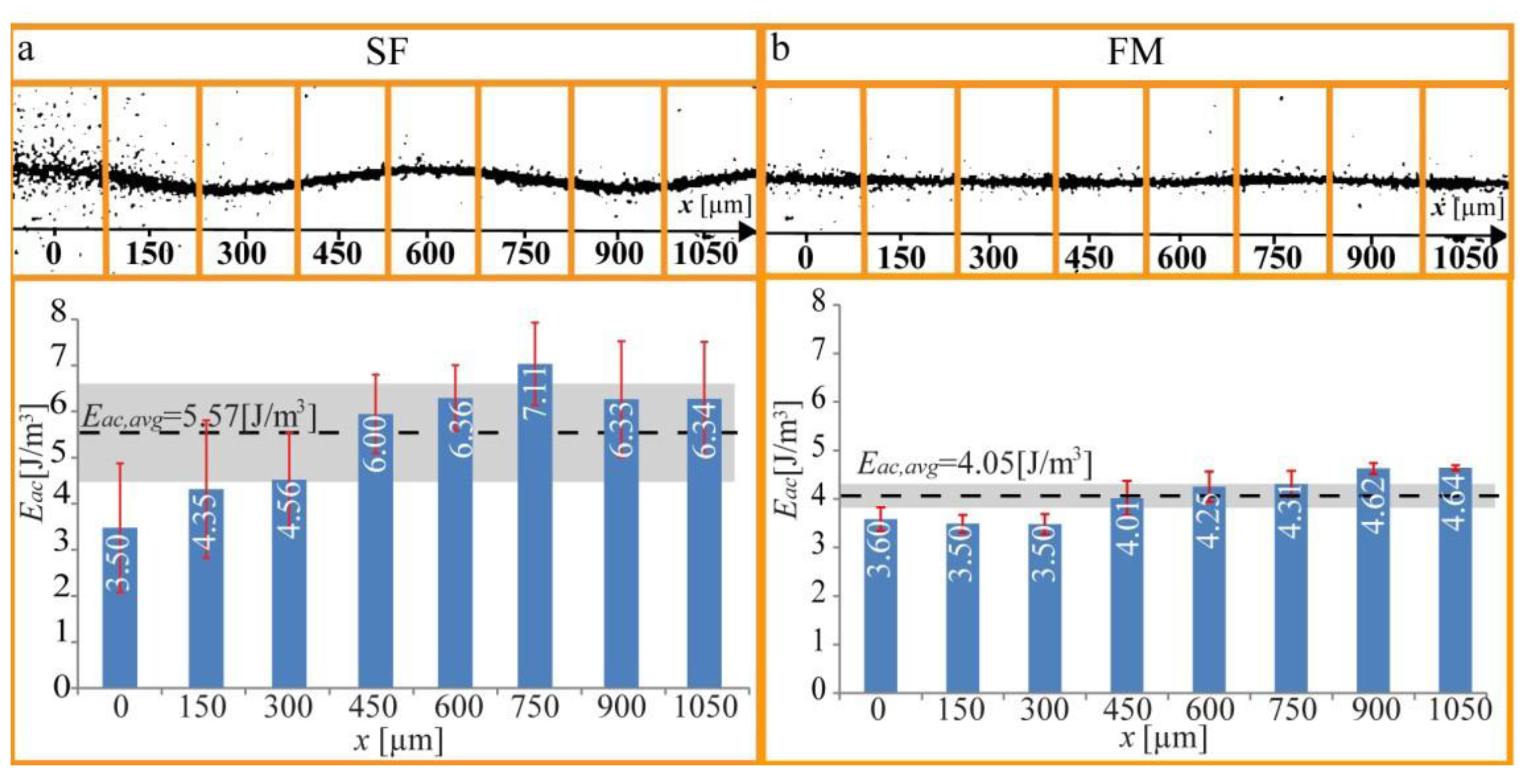
Figure 6, we demonstrate quantification of the acoustic energy density in a microchannel when it is operated at a single (optimal) frequency, and we compare with the corresponding energy density for the same (center) frequency, but with the frequency-modulation function active (100 kHz bandwidth and 1 kHz rate). As seen in the diagram, the average energy density is just slightly lower for frequency-modulation relative single-frequency actuation. This result is important since it means that there is no compromise between positioning accuracy and radiation forces when using frequency- modulation actuation instead of single-frequency actuation.
Another relatively simple and straightforward method for measuring acoustic energy density is particle tracking. This method is based on either manual or automated tracking of the position of individual particles over time. Thus, the method requires well-resolved particles and moderate particle concentrations (i.e., no particle-particle overlaps in the recorded images). The tracking data from a time sequence following a particle from its initial position into the pressure node can then be translated into a radiation force based on balancing Equation (1) with the viscous drag [
17]. This method has been used for, e.g., measuring the quality factor (
Q-value) of an acoustophoretic resonance in a microdevice by measuring the energy density as a function of the actuation frequency [
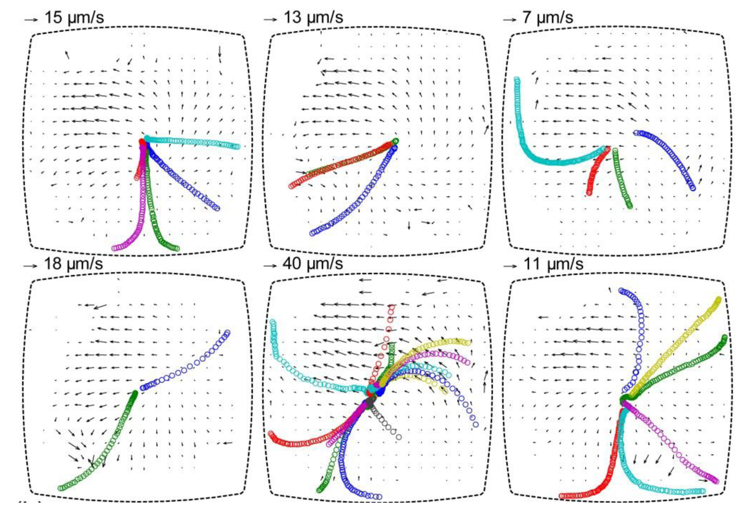
33]. For the multi-well microplate discussed in this review, particle tracking was performed for estimating the forces acting on 10 µm polystyrene particles in the wells. The particle tracks in one of the hundred wells are shown in
Figure 7 (six repetitions of the same experiment). This data containing tracks of 30 particles resulted in an acoustic energy density between 1 and 4 J m
−3, which corresponds to acoustic pressure amplitudes of 0.3–0.7 MPa, and acoustic radiation forces from 10 to 50 pN. These values are within the range of biocompatible ultrasonic manipulation of cells [
34].
Figure 6.
Measurement of the spatial distribution of the acoustic energy density along a micro-channel (
x-axis), when actuating the chip with (
a) Single-frequency (SF) actuation; and (
b) Frequency-modulation (FM) actuation. The light-intensity method was applied to eight 150
μm wide subsections of the recorded images. The averaged energy density for the whole channel,
Eac, avg, is marked with a dotted black line, and the corresponding 1
σ standard deviation is markedwith a grey band. The red error bars are the standard deviations from the four repetitions of each experiment. The figure is reproduced from Ref. [
28] by permission from IOP Publishing.
The last method, particle image velocimetry (PIV) [
35], analyzes groups of particles from recorded image sequences, rather than individual particles (as for the particle tracking method). When applied to a microsystem using a microscope, the method is often called micro-PIV. The group of particles to be analyzed is defined by a certain interrogation window in the recorded image. Two such corresponding interrogation windows from two image frames separated in time are then inserted into a cross-correlation algorithm that compares light intensities for generating a velocity vector. The full velocity vector field can be used in the same way as for the particle tracking method for calculating the acoustic radiation forces. A strength of PIV is that it allows automated analysis of complex velocity fields. However, it is a time-consuming procedure to acquire reliable PIV data [
36].
It is also possible to use PIV for measuring acoustic streaming in a microfluidic device. This has been performed in the multi-well microplate together with the particle tracking method described above. Thus, acoustic radiation forces and acoustic streaming velocities can be measured simultaneously when the two methods are combined. This is shown in
Figure 7, where the background velocity field is measured by micro-PIV using 1 µm polystyrene beads [
17]. The reason that the two methods can be combined is that the 10 µm particles are less influenced by acoustic streaming, and 1 µm particles are less influenced by the acoustic radiation force at the utilized frequency range (2–3 MHz) [
37].
Figure 7.
Particle tracking for estimation of acoustic radiation forces acting on 10 µm polystyrene particles, and particle image velocimetry (PIV) diagrams showing the background velocity field from acoustic streaming. The diagrams show the particle motion in the same well for six repetitions of the experiment after re-seeding the well with new particles. The tracks of 10 µm particles are indicated by circles (one color per individual particle), and the acoustic streaming is measured by with 1 µm particles used as flow trackers. The diagrams are based on a figure in Ref. [
17].
It is interesting to compare the three methods (light intensity, particle tracking and PIV). Light intensity has the advantage that it can be used with high particle concentrations and limited optical performance of the microscope. It does not require any advanced equipment or skillful operator, and can therefore easily be implemented in any lab. However, an optically transparent chip is needed [
28,
32]. The next method, particle tracking, is also easy to implement and it is the most suitable method for measuring the local pressure amplitude without any possible disturbance from particle-particle interactions. (Note that all three methods utilize the Gor’kov equation (Equation (1)) which assumes single particles.) However, particle tracking is time-consuming and provides low spatial resolution of the measured energy density. Finally, PIV is the most sophisticated method and can, if performed properly, provide very accurate and reliable data [
36]. However, PIV requires careful tuning of the particle concentration and image properties of the microscope, relative the input parameters in the PIV algorithms (primarily the size of the interrogation window defining the spatial resolution of the measure field). Therefore, a PIV-trained operator is needed.
